AN APPROACH TO AVOID OBSTACLES IN MOBILE ROBOT NAVIGATION:
THE TANGENTIAL ESCAPE
Andr´e Ferreira
∗Fl´avio Garcia Pereira
∗Raquel Frizera Vassallo
∗Teodiano Freire Bastos Filho
∗M´ario Sarcinelli Filho
∗∗Programa de P´os-Graduac¸˜ao em Engenharia El´etrica - Universidade Federal do Esp´ırito Santo
Av. Fernando Ferrari, 514 29.075-910 Vit´oria, ES, Brazil
ABSTRACT
An approach to guide a mobile robot from an initial position to a goal position avoiding any obstacle in its path, when nav-igating in a semi-structured environment, is proposed in this paper. Such an approach, hereinafter referred to as tangen-tial escape, consists in changing the current robot orientation through a suitable combination of the values of the angular and linear velocities (the control actions) whenever an obsta-cle is detected close to it. Then, the robot starts navigating in parallel to the tangent to the obstacle, regarding the point of the obstacle boundary the robot sensing system identifies as the closest one. The stability of the control system designed according this approach is proven, showing that the robot reaches any reachable goal, with or without a prescribed final orientation. Such a control system is programmed onboard a mobile platform whose sensing system is a laser scanner which provides 181 range measurements, for experimental validation. The results obtained are presented and discussed, allowing concluding that the tangential escape approach is able to guide the robot along trajectories that result in a re-duction of the traveling time, thus saving batteries and
reduc-Artigo submetido em 15/05/2007 1a. Revis ˜ao em 01/05/2008 2a. Revis ˜ao em 29/09/2008
Aceito sob recomendac¸ ˜ao do Editor Associado Prof. Jos ´e Reinaldo Silva
ing the motor wearing.
KEYWORDS: Tangential escape, obstacle avoidance, mobile
robot navigation, impedance-based control.
1
INTRODUCTION
Meng, 2001), and Steering Paradigm (SP) (Qu et al., 2004), have been proposed to guide the robot to accomplish such a task.
Some of such approaches are based on the deliberative paradigm, because they include a path-planning step per-formed over a previously known map of the robot work-ing environment (global trajectory plannwork-ing). The VFH, the VFF, the Certainty Grid, the CVM, the RPD, the SP, and the Dynamic Programming are examples of deliberative ap-proaches. They use a previously known detailed map of the environment surrounding the robot to plan the entire trajec-tory it should follow to reach the goal. These approaches, however, loose effectiveness if an unpredicted obstacle ap-pears in the robot path: as it was not included in the environ-mental map, it is not possible to guarantee that a collision will not occur. To deal with unpredicted obstacles, some deliber-ative approaches, like those in (Lamiraux et al., 2004), (Qu et al., 2004), (Belkhouche and Belkhouche, 2005), (Minguez and Montano, 2004b) and (Belkhous et al., 2005), have pro-posed different ways to temporarily change the planned tra-jectory. Anyway, such strategies demand an initial path plan-ning step, thus being not strictly deliberative approaches, but hybrid approaches.
Other approaches to avoid obstacles are based on the reac-tive paradigm, whose basic assumption is that the robot has no a priori knowledge about the environment surrounding it. Then, no global trajectory is planned, since a map of the robot working environment is not available. The result is a control system entirely based on the statement “per-ceptions are tightly related to actions”, meaning that the robot simply reacts according to its perception of the envi-ronment surrounding it. As a consequence, reactive navi-gation is closely related to control architectures demanding low computational effort. Changes in the environment are not a problem as well: the robot is able to perceive any environmental change and to react to it. Therefore, reac-tive navigation is more suitable to weakly structured envi-ronments, while deliberative navigation is more suitable to strongly structured environments. Edge Detection (Kuc and Barshan, 1989) and Potential Field (Khatib, 1986), among the classical approaches, as well as the approaches proposed in (Yang and Meng, 2001), (Minguez and Montano, 2004a) and (Yagi et al., 2001) are strictly reactive approaches.
This paper revisits the problem of obstacle avoidance in mo-bile robot navigation, and proposes a strictly reactive ap-proach, the tangential escape, to make the robot to reach a pre-defined goal avoiding any obstacle in its path. In the essence, the approach here proposed is different from other approaches recently proposed to guide the robot to accom-plish the same task. For example, it differs from the one proposed in (Yagi et al., 2001) for demanding a much
sim-pler feature extraction, regarding the sensorial data collected. In comparison with the approach proposed in (Minguez and Montano, 2004a), an advantage of the approach here pro-posed is that it does not demand to identify and analyze a set (may be a big one) of possibilities before choosing one, thus allowing a faster reaction to the presence of an obsta-cle. In comparison with the approach proposed in (Yang and Meng, 2001), the computational complexity is much lower, while in comparison with the proposal presented in (Belkhouche and Belkhouche, 2005), it is not necessary to know the dimensions of the obstacles, since they are not modeled in any way.
To describe, implement and experimentally validate the tan-gential escape approach for obstacle avoidance during goal-seeking, this paper is hereinafter split in six sections. The kinematic model of the mobile robot and a control system to guide the robot to the goal in the absence of obstacles are presented in Section 2. Following, an impedance-based con-trol system (Hogan, 1985; Secchi et al., 2001; Carelli and Freire, 2003) is discussed in Section 3, because it is the base for understanding the approach here proposed. In the se-quence, Section 4 describes the essence of the tangential es-cape approach. Next, Section 5 describes the implementa-tion of the control system based on the tangential escape ap-proach, using range measurements provided by a laser scan-ner as sensorial data. Experiments run using such implemen-tation are presented and discussed in Section 6, for validating the proposed approach. Finally, Section 7 highlights the main conclusions of the work.
2
SEEKING FOR THE GOAL
The task the robot should accomplish, to seek for a goal avoiding any obstacle suddenly appearing in its path, can be split in a two-steps task. The first step is to get closer to the goal (whenever there is no obstacle in the vicinity of the robot), and the second step is to change the current robot heading angle to avoid the nearest obstacle (when obstacles are detected in the vicinity of the robot). After the robot leaves an obstacle behind, the first step is resumed, and the distance between the robot and its goal is continuously re-duced, until it reaches such goal (after having avoided all the obstacles in its path).
Xc Y
c <a>
<g>
Xd
Y d
X Y
u
Figure 1: The mobile robot seeking for the goal< g >.
2.1
The Kinematic Model of the Robot
The kinematic model of the mobile robot used in the exper-iments here reported is now discussed. The mobile robot is an unicycle-like differential drive platform whose con-trol signals are the linear and angular velocities (uandω). A sketch of the robot navigating towards its goal in a free space is given in Figure 1. The mathematical model describ-ing this navigation, in polar coordinates, is given by (Secchi et al., 2001)
˙
ρ = −ucosα,
˙
α = −ω+usinα
ρ , (1)
˙
θ = usinα ρ ,
whereρis the distance robot-goal, which is the origin of the inertial frame of coordinates< g >,uis the linear velocity of the robot (in the direction normal to the axis linking its driven wheels),ω is the angular velocity of the robot, αis the orientation error (regarding the goal position), θ is the angle between the line linking the origins of the onboard and the inertial frames of coordinates and the horizontal axis, and Ψis the angle between the direction of movement and the horizontal axis.
Notice thatρshould be a nonzero value. Otherwise, it would cause the values of αandθ to be undefined. This way, it is considered that the robot reached the goal whenρ ≤ δ, whereδ > 0is a user-defined small value. In other words, the robot never reaches the goal itself, but gets as close of it as one wants. Hence, whenever mentioning that the robot
reaches the goal, hereinafter, one should understand that the robot is inside a circle of radiusδcentered in the goal.
2.2
Controlling the Position Error
From the model presented in Figure 1, one can see that the robot can be fully controlled through the values ofuandω. Despite this, this work just deals with the problem of con-trolling the robot in such a way thatρ→0andα→0(for a control law that includes the conditionθ →θd the reader
can see (Secchi et al., 2001)). The reason for considering such control law is that it is enough to allow understanding the approach here proposed to avoid obstacles.
Thus, the objective of the control system is to make the state variablesρandαto asymptotically go to zero. For checking such a condition, one can consider the Lyapunov function candidate
V(ρ, α) =1 2ρ
2
+1 2α
2
, (2)
whose temporal derivative ˙
V(ρ, α) =ρρ˙+αα˙ (3)
should be non-positive.
Regarding the robot kinematic model in (1), the value of ˙
V(ρ, α)becomes
˙
V(ρ, α) =−ρucosα+α(−ω+usinα
ρ ), (4)
and is negative definite if the control variablesuandω are defined as
u = umaxtanhρcosα,
ω = kωα+umax
tanhρ
ρ sinαcosα, kω>0,
thus demonstrating the asymptotic convergence of
ρ α
to 0 0
. This means that the robot always reaches its goal (supposed to be a reachable one) in the absence of ob-stacles.
In order to complete this stability analysis, it is important to check the behavior ofθ. Although not being controlled, it is possible to verify thatθ˙ →0whent → ∞. In order to do that, one should first take the value ofα˙ from (1) and con-sider the values ofωandu. This would result in the equation
˙
α+kωα= 0, whose solutionα=α0e−kωtshows thatα(t) is a bounded function and thatα→0whent→ ∞. Now, re-garding the value ofθ˙in (1) and the equation that defines the value ofu, one getsθ˙=umax
tanhρ
ρ sinαcosα. From such
which shows that the robot reaches the goal without oscilla-tions in any of the variables of interest, although the arriving angleθis not defined (although being a constant one).
Regarding the equation definingu, one can notice the use of the function tanh, whose objective is to saturate the value of
uto the maximum value umax, a value obtained from the
data sheet of the robot. Regarding the equation that defines the value of the angular velocityw, by its turn, one can no-tice that such a value is also saturated. This maximum value corresponds to ∂ω∂α = 0, considering that tanhρ
ρ ≃ 1 when
ρ→0. This results in the value|ωmax|=kωπ4 + 0.5umax,
which can also be obtained from the data sheet of the robot. Notice that from such value of |ωmax| the value of kω is
straightforwardly obtained, thus concluding the synthesis of the controller.
The control system proposed to guide the robot to reach the goal in the absence of obstacles is given by the inner control loop in Figure 3 and in Figure 8, where the vectorX~d =
xd yd defines the coordinates of the goal position and
the vectorX~c= xc yc , obtained through odometry (as
well as the angleΨ), defines the coordinates of the current robot position.
3
THE IMPEDANCE-BASED CONTROL
Impedance-based control is a popular technique to avoid ob-stacles. It adopts a quite simple strategy, thus resulting in fast reaction to the presence of obstacles, what makes it a very interesting approach. It makes use of the concept of general-ized or extended impedance to characterize the relationship between a mobile robot moving towards an obstacle and a fictitious repulsion force (Hogan, 1985; Secchi et al., 2001) proportional to the distance between the robot and the obsta-cle. Thus, the objective of avoiding the robot-obstacle con-tact is accomplished if the repulsion force increases when the robot gets closer to the obstacle.
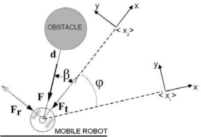
Figure 2 shows a situation in which an obstacle is detected by the robot sensors. The repulsion forceF~ is then generated, which causes the temporary displacement of the goal point
Xd, as illustrated. As a result of seeking for the new goal,
a change is imposed to the heading angle of the robot, thus allowing it to deviate from the obstacle. The components of the forceF~ (F~t, aligned to the axis of movement of the robot,
andF~r, perpendicular to it) are also represented.
The magnitude F of the repulsion forceF~ the obstacle exerts on the robot is calculated as (Secchi et al., 2001)
F =a−b(d−dmin)
2
, (5)
whereaandbare positive constants satisfying the condition
a=b(dmax−dmin)
2
,dminis the minimum measurable
dis-Figure 2: The fictitious repulsion force caused by an obsta-cle.
tance (characteristic of the sensing system),dmaxis the
max-imum distance that causes a nonzero repulsion force (speci-fied by the user), anddis the smallest distance between the robot and the obstacle delivered by the set of sensors (notice thatdmin < d < dmax). The bounddmaxcharacterizes the
repulsion zone, which is the region inside which the fictitious repulsion force has a non-zero value. An impedance
Z(s) =Bs+K (6)
is then defined, whereB andK are positive constants em-ulating the damping and the spring effects, respectively, in-volved in the robot-obstacle interaction inside the repulsion zone. Then, an impedance errorxacaused by the forceF~tof
magnitudeFt(see Figure 2) is calculated as the solution of
the equation
Ft=Bx˙a+Kxa, (7)
while the angleϕthat causes the rotation of the goal position
~
Xdis given by
ϕ=xasign(Fr). (8)
The constantsBandKare calculated in such a way that the control system is critically damped.
Finally, the goal positionX~dis rotated to the temporary
po-sition
~ Xr=
cosϕ sinϕ
−sinϕ cosϕ
~
Xd, (9)
which becomes the new reference to the position error con-troller (see Subsection 2.2). This control loop is then re-sponsible for taking the robot to the new goal, as shown in Figure 3. The control signalsuandω in such a figure are the robot linear and angular velocities, respectively, while
~
Xc = [ xc yc ]is the current robot position, in cartesian
Figure 3: Block diagram corresponding to the impedance-based control.
Therefore, whenever an obstacle is detected inside the repul-sion zone a fictitious forceF~ is generated, which causes a non-zero rotation angleϕ, thus making the robot to avoid the obstacle (the external loop of Figure 3). Otherwise, the angle
ϕbecomes zero, thus allowing the robot to continue to seek for the effective goalX~d.
Finally, it is worthy to emphasize that this control system is stable in the Lyapunov sense, as demonstrated in (Secchi et al., 2001), thus meaning that the robot will always reach the goal (supposed to be reachable) after escaping of all ob-stacles.
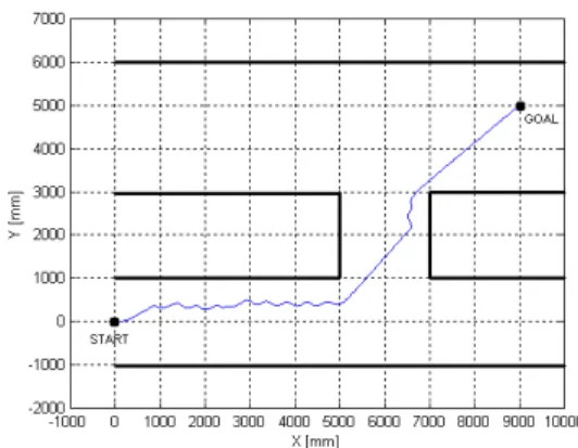
Following, a simulation of an impedance-based control sys-tem designed to guide the robot to a goal avoiding any obsta-cles in its path is presented, which was performed using the simulator of the ActivMediaP ioneerr2-DX mobile robot,
with the goal positioned in (9000 mm, 5000 mm). Figure 4 shows the path followed by the robot from the starting point (0 mm, 0 mm) (in which the angleΨ = 0 degrees) to the
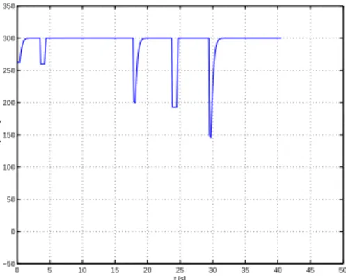
destination point (the orientation of the robot when reaching the goal is not taken into account), as well as the environ-ment configuration (the darker lines). The environenviron-ment is a set of three corridors, whose walls are the obstacles the robot should avoid. When an obstacle is detected, a fictitious repul-sion force is generated and the robot makes a turn. The value ofdmax was chosen to be70cm. Figure 5 shows the
con-trol signalugenerated by the position error controller. From such figure one can notice meaningful variations in the robot linear velocity, which mean great accelerations and deceler-ations of the robot motors. Besides such a variation in the linear velocity, one should notice that the angular velocityω
exhibits oscillations, as shown in Figure 6. Actually, such os-cillations are quite common in systems based on the concept of potential fields approach (Koren and Borenstein, 1991), as it is the case of the impedance-based control.
4
THE PROPOSED APPROACH
A new approach to guide the robot when avoiding obstacles is now proposed, whose essence is to choose a escape path
Figure 4: The path followed by the robot with the impedance-based controller.
0 5 10 15 20 25 30 35 40 45 50
−50 0 50 100 150 200 250 300 350
t [s]
u [mm/s]
Figure 5: The linear velocity of the robot with the impedance-based controller.
0 5 10 15 20 25 30 35 40 45 50 −100
−80 −60 −40 −20 0 20 40 60 80 100
t [s]
w [deg/s]
Figure 6: The angular velocity of the robot with the impedance-based controller.
which is determined by the position of the sensor that gives the least range measurement, regarding a set of sensors able to perform range measurement, as a laser scanner, for exam-ple. The rotation angle is now determined so that after ma-neuvering the vehicle takes the direction of the tangent to the boundary of the obstacle in that point. The advantage is that the robot performs smoother movements when navigating, as it is shown in the sequence.
Therefore, whenever an obstacle is detected inside the repul-sion zone defined by the distancedobs(see Figure 7), the
an-gleβ is determined, from the range measurements provided by the onboard sensing system. Such an angle is defined by the direction in which it was gotten the minimum range mea-surement, and is related to the characteristics of the sensing system. For example, if the sensing system is a ring of ultra-sonic sensors, such an angle is obtained from the disposition of the sensors in the ring, in relation to the axis of movement of the robot. Knowing the robot orientation relative to the real target (the angleα) and estimating the angleβ, the angle
ϕthat allows the tangential escape is obtained as
ϕ=sign(β)π
2 −(β−α), (10) whereα > 0 when the obstacle is at the right of the axis of movement of the robot andβ > 0when the obstacle is detected at the right side of the robot. In this configuration, which is depicted in Figure 7, the angleϕis positive, mean-ing that the real goal is rotated to the left side, regardmean-ing the axis of movement of the robot.
The angleϕis then used in the rotation matrix in (9), and the real goal is rotated to a new position (the virtual goal). The position error controller starts using the coordinates of the virtual target, causing the robot to take the tangent to the obstacle boundary. Notice that in the absence of obstacles there is no change in the position of the real goal, and the
Obstacle Avoidance Zone
d
obsd
minβ
ρ
θ
α
γ
Real GoalVirtual Goal
Figure 7: Obtaining the angleϕ.
robot continues seeking for it. A control system implement-ing the tangential escape approach is sketched in Figure 8, whereu,ωand the vectorX~c have the same meaning as in
Section 3. This way, regarding the asymptotic stability of the position error controller, it is straightforward to conclude that the control system implementing the tangential escape is also asymptotically stable, which guarantees that after escaping of all obstacles the robot always reaches its goal (supposed to be reachable).
In order to evaluate how the control system based on the tangential escape approach performs, a simulated example is now presented. The objective is to take the robot from the starting point (0 mm, 0 mm) (with orientation Ψ =
0 degrees) to the goal point (9000 mm, 5000 mm) once
more, avoiding any obstacle in its path. Notice that this is the same example simulated using the impedance-based control in Section 3, and the walls of the three corridors are the obsta-cles to be avoided. Figure 9 shows the path the robot traveled over to reach the goal. Whenever an obstacle (a wall of a cor-ridor the robot entered in) is detected, the robot turns around in order to follow a line parallel to it. The distancedobsthat
defines the repulsion zone was defined as70cmonce more. Complementing the simulated example, Figure 10 shows the linear velocity developed by the robot along its path, while Figure 11 shows its angular velocity.
Figure 8: Block diagram of the control system based on the tangential escape approach.
Figure 9: The path the robot traveled over with the tangential escape approach.
of the fact that the average linear velocity the robot devel-ops is greater, because of the absence of the frequent de-celerations associated to the oscillations present in Figure 4. Therefore, the tangential escape approach is very attractive, as one can see from the simulations presented. In addition, the simulated example itself shows that the tangential escape approach for obstacle avoidance gives the robot the capabil-ity of navigating in environments somewhat complex using a single controller, differently of the work reported in (Carelli and Freire, 2003), for example.
5
IMPLEMENTING THE TANGENTIAL
ES-CAPE APPROACH
The key point of the tangential escape approach is the es-timation of the anglesαandβ. The first one is recovered from the robot odometry, as the robot knows its current po-sition and the popo-sition of the goal it is seeking for (see Fig-ure 7). By its turn, the angleβis obtained from the distances robot-obstacle delivered by the sensorial apparatus onboard the robot in a certain instant.
In this section, an implementation of the control system
0 5 10 15 20 25 30 35 40 45 50
−50 0 50 100 150 200 250 300 350
t [s]
u [mm/s]
Figure 10: Robot linear velocity with the tangential escape approach.
0 5 10 15 20 25 30 35 40 45 50
−100 −80 −60 −40 −20 0 20 40 60 80 100
t [s]
w [deg/s]
Figure 11: Robot angular velocity with the tangential escape approach.
based on the tangential escape approach is programmed in the computer onboard aP ioneerr2-DX, which is fully
(a) The mobile robot used, with the onboard laser scanner.
Frist Value (−90°) Last Value
(90°)
Obstacle
(b) The range measurements obtained.
Figure 12: The experimental setup adopted.
measurements are given in Figure 12. From the figure one can realize that such a laser scanner is equivalent to 181 range sensors distributed around a semi-circle over the front of the robot platform, in intervals of 1 degree. Thus, the angleβ
stays in the interval[0degrees,180degrees], which is here transformed to the interval[−90degrees,+90degrees], for regarding obstacles in the right side (β >0) or in the left side (β <0)of the robot. With the sensing system used, however, no obstacles can be detected in the rear of the robot.
6
EXPERIMENTAL RESULTS
Two experiments were run using the control system designed to implement the tangential escape approach, which was pro-grammed onboard theP ioneerr 2-DX robot. Both
exper-iments correspond to the same example simulated in Sec-tion 4, with the difference that in the second one two circular obstacles were put in the middle of the first and second cor-ridors the robot should enter in before reaching the goal. For the first experiment, the path the robot traveled over and its angular and linear velocities along the navigation time are shown in Figure 13. For the second one, the navigation in a set of corridors containing additional obstacles, just the path the robot traveled over is presented (see Figure 14).
When analyzing the results of these experiments, one can see that those corresponding to the first experiment are very close
−1000 0 1000 2000 3000 4000 5000 6000 7000 8000 9000 10000
−2000 −1000 0 1000 2000 3000 4000 5000 6000 7000
X [mm]
Y [mm]
START
GOAL
(a) The path the robot traveled over.
0 10 20 30 40 50 60
−80 −60 −40 −20 0 20 40 60
t [s]
w [deg/s]
(b) The angular velocity the robot develops.
0 10 20 30 40 50 60
0 50 100 150 200 250 300
t [s]
v [mm/s]
(c) The linear velocity the robot develops.
−1000 0 1000 2000 3000 4000 5000 6000 7000 8000 9000 10000 −2000
−1000 0 1000 2000 3000 4000 5000 6000 7000
X [mm]
Y [mm]
GOAL
START
Figure 14: Laser-based navigation in a set of corridors with obstacles.
to the results of the simulation, as expected (see the traveled paths presented in Figures 9 and 13(a)). Other meaningful feature is the absence of oscillations in the robot trajectory when it approaches an obstacle, when adopting the tangen-tial escape approach, differently of what occurs in connection to the impedance-based control system (see Figures 4 and 13(a)). It can also be observed that the robot can get closer to an obstacle than the distancedobsdefining the repulsion
zone, as it is clear in Figure 14. Actually, the repulsion zone defines the limiting distance above which the obstacle does not cause any reaction, not the minimum distance the robot should keep between it and any obstacle. Indeed, if this were the case, the robot would not pass between the wall and the obstacles present in the corridors of Figure 14. Besides, the experiments also confirm the advantage of the tangential es-cape approach in terms of the higher average linear velocity developed by the robot and the absence of unnecessary ma-neuvers (absence of oscillations). Last, but not least, it is important to mention that the control system implementing the tangential escape is able to guide the robot when follow-ing a wall, as it can be observed in the experiments reported. However, it should be emphasized that this is completely dif-ferent from other wall-following proposals, like the one in (Carelli and Freire, 2003), for example. There, two distinct controllers are used, one for wall-following and other for ob-stacle avoidance, while in this work just one controller is re-sponsible for both behaviors, thus making it much simpler to design and faster to compute. Other wall-following ap-proaches, like the one reported in (Bemporad et al., 2000), however, are not even related to the tangential escape ap-proach, for they did not include neither goal-seeking nor ob-stacle avoidance.
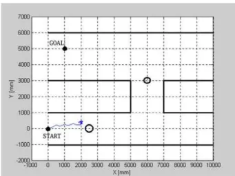
For the sake of comparison, the same experiments two were run using the impedance-based control system programmed in the sameP ioneerr2-DX robot. In the first one the robot
reached the goal without major problems, but in the second
Figure 15: Navigation in a set of corridors having obstacles, using the impedance-based controller.
one it did not manage to go beyond the obstacle in the first corridor, as shown in Figure 15. Then, one gets the conclu-sion that the proposed approach is effectively much better than the impedance-based control, in terms of avoiding ob-stacles, energy consumption, time to get the goal and motor wearing.
Finally, it is worthy to mention that the figures showing the path the robot traveled over in the experiments are built with data recovered through the robot odometry. Then, as it is well known from the literature, the real final position reached by the robot is somewhat different from the ideal one, due to odometric errors. Indeed, those errors are present in Fig-ures 13(a) and 14.
To close the experimentation, an experiment similar to the second one above analyzed was run, using the same
P ioneerr 2-DX robot having the same laser scanner
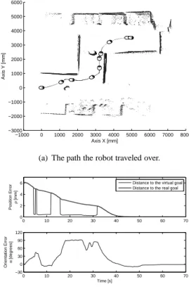
on-board and running a controller based in the tangential escape approach in its onboard computer. The results are shown in Figure 16, with the characteristic that the environment sur-rounding the robot was built using the range measurements collected during the navigation. In addition to the path the robot traveled over (Figure 16(a)), the position and orienta-tion errors (Figure 16(b)) and the linear and angular veloci-ties sent to the robot by the controller and effectively devel-oped by the robot (Figure 16(c)) are also presented. From such figures one can see that the control system effectively drives the robot till reaching the goal and stopping there, as
ρ→0,α→0,u→0andω→0.
−1000 0 1000 2000 3000 4000 5000 6000 7000 8000 −3000
−2000 −1000 0 1000 2000 3000 4000 5000 6000
Axis X [mm]
Axis Y [mm]
(a) The path the robot traveled over.
0 10 20 30 40 50 60 70 0
2 4 6
Position Error
ρ
[mm]
0 10 20 30 40 50 60 70 −30
0 30 60 90 120
Time [s]
Orientation Error
α
[degrees]
Distance to the virtual goal Distance to the real goal
(b) The evolution of the position and orientation errors regard-ing the goal position.
0 10 20 30 40 50 60 70
−100 0 100 200 300 400
Linear Velocity
u [mm/s]
0 10 20 30 40 50 60 70
−45 −30 −15 0 15 30 45
Angular Velocity
ω
[rad/s]
Time [s]
ωsent
ωdeveloped
usent
udeveloped
(c) The angular and linear velocities sent to the robot and ef-fectively developed by it.
Figure 16: Another experiment considering the laser-based implementation of the tangential escape approach. Here the environment surrounding the mobile robot is built from the range measurements collected during the navigation.
linear and angular velocities it effectively develops, mainly during the maneuvers to avoid obstacles. This means that for high velocities (one should remember the limitation corre-spondent to the maximum linear and angular velocities the robot can develop), the decelerations correspondent to the evasive maneuvers and the accelerations after leaving the ob-stacle behind, excite the robot dynamics, thus meaning that for allowing the robot to develop higher velocities it would be recommendable to consider the robot dynamics, which is not done here (only the robot kinematics is considered here). However, there is no difference, in terms of the strategy here proposed for obstacle avoidance, if the maximum velocities the robot is allowed to develop are higher or lower.
7
CONCLUSION
A novel approach is here proposed to avoid obstacles when a mobile robot is seeking for a goal, which is referred to as the tangential escape. The essence of the method is to make the robot to follow the direction of the tangent to the obstacle boundary in the point that is closest to it, whenever an obsta-cle is detected closer to the robot than a specified distance.
The control system thus implemented is shown to be stable in the Lyapunov sense, which means that a reachable goal is always reached. Two experiments using an implementation of the tangential escape approach based on the range mea-surement provided by a laser scanner have shown that it is effectively able to guide the robot to the goal without col-liding to any obstacle, thus validating the proposed method. Moreover, such experiments have also shown that the con-trol system based on the tangential escape approach can re-duce the traveling time, the energy consumption and the mo-tor wearing, for avoiding unnecessary acceleration and de-celeration associated to unnecessary maneuvers. This way, the tangential escape approach is a very attractive one to deal with goal-seeking and obstacle avoidance, as it is shown in the paper.
Finally, besides its simplicity and effectiveness, it should be emphasized that just one control system based on the tan-gential escape approach allows guiding the robot to navigate in environments somewhat complex, as the experiments re-ported in the paper have shown. Thus, it is not necessary to adopt distinct controllers to perform wall following and ob-stacle avoidance, for example.
ACKNOWLEDGEMENTS
REFERENCES
Belkhouche, F. and Belkhouche, B. (2005). A method for robot navigation toward a moving goal with unknown maneuvers, Robotica 23(6): 709–720.
Belkhous, S., Azzouz, A., Saad, M., Nerguizian, C. and Ner-guizian, V. (2005). A novel approach for mobile robot navigation with dynamic obstacles avoidance, Journal
of Inteligent Robotic Systems 44(3): 187–201.
Bemporad, A., di Marco, M. and Tesi, A. (2000). Sonar-based wall-following control of mobile robots, ASME
Journal of Dynamic Systems, Measurement and Control
122(1): 226–230.
Borenstein, J. and Koren, Y. (1989). Real-time obstacle avoidance for fast mobile robots, IEEE Transactions on
Systems, Man, and Cybernetics 19(5): 1179–1187.
Borenstein, J. and Koren, Y. (1991). The vector field histogram - fast obstacle avoidance for mobile robots, IEEE Transactions on Robotics and Automation 7(3): 278–288.
Carelli, R. and Freire, E. O. (2003). Corridor navigation and wall-following stable control for sonar-based mo-bile robots, Robotics and Autonomous Systems 45(3-4): 235–247.
Elfes, A. (1987). Sonar-based real-world mapping and navi-gation, IEEE Journal of Robotics and Automation RA-3(3): 249–265.
Hogan, N. (1985). Impedance control: An approach to ma-nipulation, ASME Journal of Dynamic Systems,
Mea-surement, and Control 107: 1–23.
Khatib, O. (1986). Real time obstacle avoidance for manip-ulators and mobile robots, The International Journal of
Robotics Research 5(1): 90–98.
Koren, Y. and Borenstein, J. (1991). Potential field methods and their inherent limitations for mobile robot naviga-tion, Proceedings of the IEEE Conference on Robotics
and Automation, Sacramento, California, pp. 1398–
1404.
Kuc, R. and Barshan, B. (1989). Navigating vehicles through an unstructured environment with sonar, Proc. of the
1989 IEEE International Conference on Robotics and Automation, Vol. 3, Scottsdale, AZ, pp. 1422–1426.
Lamiraux, F., Bonnafous, D. and Lefebvre, O. (2004). Reac-tive path deformation for nonholonomic mobile robots,
IEEE Transactions on Robotics 20(6): 967–977.
Minguez, J. and Montano, L. (2004a). Nearness diagram (nd) navigation: collision avoidance in troublesome scenar-ios, IEEE Transactions on Robotics and Automation 20(1): 45–59.
Minguez, J. and Montano, L. (2004b). Sensor-based robot motion generation in unknown, dynamic and trouble-some scenarios, Robotics and Autonomous Systems 52(4): 290–311.
Qu, Z., Wang, J. and Plaisted, C. E. (2004). A new ana-lytical solution to mobile robot trajectory generation in the presence of moving obstacles, IEEE Transactions
on Robotics 20(6): 978–993.
Secchi, H., Carelli, R. and Mut, V. (2001). Discrete sta-ble control of mobile robots with obstacles avoid-ance, Proc. of the 11th International Conference on
Advanced Robotics, ICAR’01, Budapest, Hungary,
pp. 405–411.
Willms, A. R. and Yang, S. X. (2006). An efficient dynamic system for real-time robot-path planning, IEEE
Trans-actions on Systems, Man and Cybernetics - Part B: Cy-bernetics 36(4): 755–766.
Yagi, Y., Nagai, H., Yamazawa, K. and Yachida, M. (2001). Reactive visual navigation based on omnidirectional sensing - path following and collision avoidance,
Jour-nal of Intelligent and Robotic Systems 31(4): 379–395.
Yang, S. X. and Meng, M. (2001). Neural network ap-proaches to dynamic collision-free trajectory genera-tion, IEEE Transactions on Systems, Man and