Two-Sector Representative Consumer
Economy
∗
Orlando Gomes
†
Contents: 1. Introduction; 2. A Multiple Research Projects Two-Sector Model; 3. Dynamics and Steady-State Properties; 4. Growth-Paths: A Numerical Example; 5. Discussion – Heterogeneous Researchers and Endogenous Fluctuations; 6. Conclusions; A. Proof of Propositions; B. Numerical Example Time Trajectories.
Keywords: Heterogeneous agents; Bounded rationality; Optimal control; Research activities; Volatility and chaos.
JEL Code:C61; O32; O33.
Research activities have uncertain outcomes. The question asked in this paper is whether or not this uncertainty can be a central piece on the expla-nation of long run consumption growth paths. More specifically, we inquire how the existence of different research projects, with different degrees of uncertainty, contributes to unpredictable consumption growth paths. The proposed scenario is a two-sector representative consumer model with re-searchers that invest in different innovation projects. There is heterogene-ity in terms of risk associated to research programs (researchers invest in projects with the same expected outcome but different volatility). This difference in volatility, combined with an adaptive learning – bounded ra-tionality rule, implies an aggregate index of technology and a consumption growth rate that do not present a predictable pattern over time.
As actividades de investigação produzem resultados incertos. A questão colocada neste artigo é se esta incerteza pode ser uma peça central na expli-cação das trajectórias de crescimento do consumo no longo prazo. Mais es-pecificamente, pergunta-se como a existência de diferentes projectos de inves-tigação, com diferentes graus de incerteza associados, contribui para trajec-tórias de crescimento do consumo que não são passíveis de previsão. O cenário
∗Financial support from the Fundação Ciência e Tecnologia, Lisbon, is grateful acknowledged, under the contract No
POCTI/ECO/48628/2002, partially funded by the European Regional Development Fund (ERDF). I also acknowledge the im-portant comments made by an anonymous referee and the helpful assistance of the journal’s editors. The usual disclaimer applies.
†Escola Superior de Comunicação Social [Campus de Benfica do Instituto Politécnico de Lisboa; 1549-014 Lisboa, Portugal] and
proposto é um modelo de consumidor representativo de dois sectores com in-vestigadores que investem em diferentes projectos de inovação. Existe hetero-geneidade ao nível do risco associado aos programas de investigação (os inves-tigadores investem em projectos com o mesmo resultado esperado mas diferente volatilidade). A diferença na volatilidade, combinada com uma regra de apren-dizagem adaptativa – racionalidade limitada, implica um índice agregado de tecnologia e uma taxa de crescimento do consumo que não apresentam um padrão previsível ao longo do tempo.
1. INTRODUCTION
Heterogeneity regarding economic agents beliefs and behavior is an important field in today’s eco-nomic research. The most influential work at this level respects to the explanation of asset prices fluctuations. Starting with the work of Brock and Hommes (1998), several authors have tried to ex-plain how the co-existence of fundamentalist traders and technical analysts contributes to a random and hardly predictable time series for asset prices. In this kind of asset pricing models, heterogeneity combined with an adaptive belief system allows to find time paths for asset prices that are erratic, that is, where periods of low volatility and high volatility alternate, where volatility clustering is evidenced and where some important empirical features about financial markets can be mimetized. Some impor-tant work concerning asset pricing heterogeneous agents was developed in Brock et al. (2001), Hommes et al. (2002), Gaunersdorfer et al. (2003), Azariadis and Kaas (2002), Chiarella and He (2002), Kurz and Schneider (1996), Kurz (1997a), Kurz and Beltratti (1997) and Kurz and Motolese (2001).
Heterogeneity and adaptive beliefs are also an influential line of thought of contemporary macroe-conomics, mainly in what concerns expectations and learning mechanisms. The most important ref-erences at this level are, on one hand, the bounded rationality approach of Sargent (1993) and the discussion of learning mechanisms by Evans and Honkapohja (2001). Other authors, like Barucci (1999), Nourry and Venditti (2001), Tuinstra and Wagener (2003) and Negroni (2003) study stability conditions of macroeconomic models with heterogeneous agents.
Heterogeneity analysis is today extended to a large number of economic issues. Besides asset pric-ing and macroeconomic stability, different individual behavior or expectations serves as a means to explain exchange rate fluctuations [De Grauwe and Grimaldi (2002)], economic growth [Maliar and Maliar (2001), Becker and Tsyganov (2002)] or monetary policy [Kurz et al. (2003)].
The model to develop in this paper combines, as the previous references, a mechanism of bounded rationality and learning with the notion of agent heterogeneity. This model is an endogenous growth two sector model where a representative consumer maximizes utility. The source of heterogeneity is in technology generation [as in Kurz et al. (2003)] and not in consumer preferences as it became usual in this kind of model [it is the case of Becker and Tsyganov (2002)] – the representative consumer structure continuous to hold. Under such a scenario we observe that different risk in R&D activities can explain long run consumption growth rates that are erratic and impossible to predict.
to accumulated past results concerning the innovation activity, such that in certain periods of time it increases and in others it declines.
The fundamental result is that heterogeneity in one economic sector is a source of randomness and unpredictability for the whole economic system. The production of final goods may not be associated to unpredictable outcomes, at least not in the same extent as the generation of knowledge, but final goods time trajectories become erratic trajectories in the moment that we consider a technological level that is determined by the dynamics of a heterogeneous agents – bounded rationality research sector.
The remainder of the paper has the following contents. Section 2 characterizes the main features of the model. A two-sector model is constructed, where the first sector generates a homogeneous final good that can be indistinctly consumed or used in subsequent periods as capital, and the second sector is an R&D sector. Section 3 assumes a steady state scenario with no volatility. In this case the prop-erties of the model are the ones common to the Romer-Jones endogenous growth model. In section 4 the dynamic analysis of the model is pursued through a numerical example. We understand with this example that a same set of parameters and initial values implies time paths of the most important economic aggregates that change each time the example is run. Section 5 discusses why is the present analysis relevant; in particular, it addresses the macroeconomic business cycles / endogenous fluctua-tions literature to motivate both theoretically and empirically the undertaken analysis. We argue that our model is a special case of a real business cycle framework, where technology shocks are replaced by a systematic effort of generating technical knowledge (an effort that comes from a large set of indepen-dent, autonomous and heterogeneous researchers). Finally, section 6 makes a few final comments. Two appendixes are also included: appendix A concerns to the proof of the propositions presented in section 3, while appendix B is destined to the presentation of the most important time paths of the numerical example in section 4.
2. A MULTIPLE RESEARCH PROJECTS TWO-SECTOR MODEL
We begin by assuming a discrete time infinite horizon utility maximization problem for a given
representative consumer. In this problem, variable ctdenotes the level of real consumption in each
time moment,ρ > 0is a constant discount factor andU(ct)will represent the utility function. The utility function respects the following assumptions,
i) U is continuous, concave and smooth (infinitely many times continuously differentiable);
ii) θ >1is a concavity parameter of the utility function that obeys the conditionU′
=c−θ t .
The optimal control problem consists on the maximization of the flow of utility functions in expres-sion (1),
∞
X
t=0
U(ct). 1
(1 +ρ)t (1)
The maximization problem is constrained by the economy’s production possibilities. Following the endogenous growth literature [in particular, Romer (1986) Romer (1990) and Jones (1995) Jones (2003)], we consider a two-sector environment where two kinds of economic goods are generated: final goods, that can be either consumed or used as capital in the generation of new goods, and technology. Variable
kt will define real per capita capital, which depreciates at a rateδ > 0, andAt will represent the technological level of the economy. The capital accumulation constraint is the following,
∆kt=At.f(kt)−ct−δ.kt,∆kt=kt+1−kt,k0given. (2)
The second sector generates technology, a non rival good that can be simultaneously used in the pro-duction of physical goods and in the generation of additional technology. We consider decreasing but positive marginal returns in the accumulation of technological knowledge [as in Jones (2003) we may interpret this statement as translating the existence of positive intertemporal technology spillovers]. Furthermore, technology generation depends solely on the previously accumulated knowledge.
There-fore, given a parameter φ ∈ (0,1), the technology production function is considered as a function
fA(A
t) =Aφt.
In a homogeneous scenario regarding technological investment opportunities, the following dy-namic rule reflects the accumulation of technological knowledge,
∆At=g.fA(At)−ω.At,∆At=At+1−At,A0given. (3)
In (3), parametergis a positive productivity parameter andωis an obsolescence rate for technology.
Our attention will focus on a setup with research heterogeneity. This means the existence of various investment alternatives regarding technology production. We assume that the economy is populated by a large number of researchers and that there are alternative research activitiesh= 1, . . . , H. The distinction between research activities in our framework will be made considering different degrees of risk involved in the innovation process, i.e., all activities share the same expected outcome but diverse levels of volatility characterize the various possible outcomes. The heterogeneity will be translated
through parameterg; we assume that different research projects imply distinct values for this
techno-logical productivity component. In this way, equation (3) splits inHequations, each one representing
the time evolution of the accumulation of technological knowledge regarding each specific innovation process,
∆Aht=ght.fA(At)−ω.Aht,∆Aht=Aht+1−Aht,Ah0given. (4)
Note that in (4) the accumulation of knowledge through a project of typehcorresponds to the
produc-tivity of all the already existent knowledge when applied to typehinnovative activity; the obsolescence
of this kind of technology contributes negatively to its accumulation.
For the productivity valueghtwe now assume that{ght, t = 1,2, . . .}is a Markov process. This Markov process is similar to the one in Kurz et al. (2003), i.e., the following dynamic rule is considered,
ln(ght+1) =λ.ln(ght) +εht+1,εht∼N(0, σ2h)iid (5)
withλa positive parameter. Note that the only source of heterogeneity is the standard deviation of
the normal distribution. Two possibilities regarding technological research will represent two different knowledge accumulation rates because the volatility associated with each project is not equal. Given
different time paths for ght, we guarantee that the accumulation ofAh through (4) differs among
investment in technology decisions; furthermore, given that such accumulation process is dependent on a Markov process we will have stochastic time paths characterizing technology values and technology growth rates.
The index of technology available to the production of physical goods is an aggregate value, which
may be thought as a weighted average of the technological level that results from each one of theH
research activities. Letnhtrepresent the share of researchers that at any time moment choose to follow
the research strategyh; then we define
At= H X
h=1
nht.Aht (6)
The fractions nhtare updated in time according to a bounded rationality rule or a learning
is adopted follows the asset pricing literature that have introduced the concept of ‘rational routes to randomness’, namely Brock and Hommes (1997, 1998). This learning rule is based on discrete choice models, in the line of Manski and McFadden (1981) and Anderson et al. (1992), which implies the fol-lowing value for the assumed share,
nht= e β.aht
H P
i=1
eβ.ait
,β≥0, h= 1, ..., H (7)
In expression (7),βis an intensity of choice parameter. It represents the degree of rationality with which
researchers choose to change the reallocation of their effort to another research project. Ifβ → ∞the
degree of rationality is maximum, that is, individuals change strategies immediately in the presence
of better results than the ones obtained with the chosen strategy. Forβ = 0, researchers will never
change strategy independently of the obtained results. We assume thatβ is a positive finite value,
representing a bounded rationality behavior for researchers.
Variablesahtare performance measures or fitness functions that translate the past performance of
the chosen research strategy. These functions have as a central property the fact that older observations are less relevant than recent observations [this follows a same kind of rule adopted in Barucci (1999) for the study of expectational stability in macroeconomic models with heterogeneous beliefs]. So, we consider a factorτ >0that discounts to the present past technological outcomes. Eachahtfunction is
then the sum of all the past technology values until some present momentT, according to (8).
aht= T X
t=0
Aht.
1
(1 +τ)T−t ,h= 1, ..., H (8)
We are now in conditions to define formally our model.
Definition 2.1(Heterogeneous researchers two-sector model). The representative consumer of the economy controls the time path of consumption in order to maximize the sequence of utility values in (1). The maxi-mization problem is subject to a capital accumulation constraint, (2), and to a series of H technology genera-tion rules, (4). Technological results vary according to a Markov process affecting technology productivity, (5), being innovation risk the source of heterogeneity. The number of researchers choosing an innovation strategy is determined by a bounded rationality rule, (7), where past results constitute the criteria underlying such choices, as indicated by (8). The level of technology that determines goods production is an average of the several technological achievements, as in (6).
3. DYNAMICS AND STEADY-STATE PROPERTIES
Definition3.1(Expected Steady State). DefiningE(ght)as the expected value of the stochastic variableght,
so thatE(ght+1) =E(ght), the expected steady state will be a long run locus in which the technology level
is a constant value and the consumption-capital ratio is also constant.1
Having in mind definition 3.1, we can prove several propositions. To do this, we first encounter the optimality necessary conditions of the problem in definition 2.1. Consider a Hamiltonian function,
a shadow-price for capital, pkt ≥ 0, and a set of co-state variables for each one of the technology
variables,pAht≥0,h= 1, . . . , H. The current-value Hamiltonian function is
ℵ(kt, Aht, ct) =U(ct) +pkt.[At.f(kt)−ct−δ.kt] + H X
h=1
pAht.
ght.fA(At)−ω.Aht
(9)
Optimality necessary conditions are:
∂ℵ ∂ct
= 0⇒c−θ
t =pkt (10)
∆pkt=ρ.pkt− ∂ℵ
∂kt
⇒∆pkt= (ρ+δ−ζ.At).pkt (11)
∆pAht=ρ.pAht− ∂
ℵ
∂Aht ⇒
∆pAht=
ρ+ω−φ.nht.A
−(1−φ)
t .
H P
i=1
git.pAit
.pAht−pkt.nht.f(kt),h= 1, ..., H
(12)
lim
t→+∞pkt.
1
(1 +ρ)t.kt= 0; t→lim+∞pAht.
1
(1 +ρ)t.Aht= 0 (13)
[transversality conditions]
For the set of equations (10) to (13), we present proposition 3.2.
Proposition3.2(Sufficient Optimality Conditions). First order optimality conditions (10 to 13) are also suffi-cient, given the Arrow and Kurz (1970) theorem, if one assumes that the following condition holds,
2.ζ.pkt. H X
h=1
(nht.z0.zh)≤φ.(1−φ).A
−(2−φ)
t .
H X
h=1
pAht.ght.nht. H X
j=1
(njt.zh.zj)
, (14)
∀z0, z1, ..., zH ∈R
The following analysis assumes that the values of parameters and variables are such that condition (14) is satisfied. The proof of proposition 3.2 is presented in appendix A, in the end of the text.
Relation (10) can be used to change (11) into a dynamic equation relating to the growth path of
consumption. We find a result that is common in endogenous growth literature,2
∆ct
ct
=1
θ.[ζ.At−(ρ+δ)] (15)
1Note, furthermore, that under the assumption of equal productivity initial values,g10=g20=. . .=g
H0, the expected values will
be identical in every time moment:E(g1t) =E(g2t) =. . .=E(gH t). While this assumption may be relevant in an analysis of transitional dynamics outside the steady state vicinity, it is not important in the steady state neighbourhood analysis that follows, because for allghtwe verify that∆E(ght) =E(ght)λ−E(ght), and, thus,E¯(g) = 1defines the long term equilibrium for any of theHresearch projects.
2Note that this is an approximated result, which is reasonable only for small changes inc
tover time (the result is exact in
The consumption growth rate in (15) would be a constant value if the technological level were constant.
Since every research project is subject to decreasing marginal returns, the expected value ofAttends
effectively to a long run steady state constant value, but the Markov process associated with the pro-ductivity of technological projects implies a consumption growth rate that would be around a constant value that does not, however, stabilize in such value. Periods of high and low volatility will alternate as the technological projects with high and low risk perform better, according to the learning process given by the bounded rationality mechanism. This fact will be highlighted in next section’s example.
Relatively to the expected steady state and the dynamics in the expected steady state vicinity, these are characterized by the following propositions (the correspondent proofs are presented in appendix A).
Proposition3.3(Expected Steady State Existence and Uniqueness). The optimal control problem in definition 2.1 has a unique expected steady state as described in definition 3.1.
Let us defineψt≡ct/kt; the unique steady state mentioned in proposition 2 is the vector (see the proof in appendix),
¯
ψ
¯
Ah
=
" (ζ+ 1/θ).A¯+θ−1
θ .δ+
1 θ.ρ hE¯(g)
ω
i1/(1−φ)
#
(16)
Expression (16) presents the steady state value of the consumption-capital ratio and the expected steady
state value of ahresearch project outcome. Note that every research project has a same steady state
expected outcome since, as regarded earlier, the long run expected productivity of each project is the same [E¯(g) = 1]. Note also thatA¯= ¯Ah,∀h= 1, ..., H, given the definition ofAtin (6).
Proposition3.4(Stability properties). The system relating to variablesψtandAhtexhibits saddle-path
sta-bility in the expected steady state vicinity, for anyh= 1, . . ., H.
Proposition 3.5 (Convergence properties). The system relating variables ψt andAhtpresents, in the
ex-pected steady state vicinity and for anyh = 1, . . ., H, a saddle trajectory characterized by an increasing consumption-capital ratio in the presence of an increasing technological level.
The three previous propositions are common to the class of two-sector models with capital constant returns and technology decreasing returns. The difference is that we have considered initially that researchers are distributed by different projects. The notion of expected steady state eliminates the importance of the existence of diverse innovation strategies, because those were distinguished only through different risk parameters. So, the research projects will all perform the same (we expect this) and consequently there are no incentives to change behavior, that is, the expected values of the shares
nhtwill be constant values. The model was in this way reduced to a one-dimension technology model,
in whichAt=n1.A1t+. . .+nH.AHt.
4. GROWTH-PATHS: A NUMERICAL EXAMPLE
The expected steady state notion reduces the heterogeneous agents model to a homogeneous setup. In this section we return to the model with different risk in technology investments and look to a numerical example, through which we perceive that the same parameter values imply an infinite set of possibilities for the technology and consumption long run growth rates.
It is important to clarify the following. The initial values of the productivity variablesght,h =
1, . . ., H, are irrelevant in terms of long run results. When considering the expected steady state
we have regarded that E¯(gh) = 1,∀h, independently of initial conditions. If one assumes that the
the result of the bounded rationality mechanism that is adopted, but an important aspect must be
taken into account – because the expected value ofE(gh)is the same for all technological projects
there is a co-existence of periods where a project performs better than others with periods where the reverse occurs. It is this process that allows the mechanism of discrete choice to produce the chaotic
behavior that the endogenous variables of the model, namely consumption, display. If someghprocess
had a higher average than the others, the correspondent accumulated technology outcome would be systematically superior and this process would dominate all the others; hence, the chaotic behavior would give place to the Markov process of the dominant project. Therefore, we should stress that it is the average value of the Markov processes relating productivity that triggers the chaotic behavior we observe (if the average values are equal or not too different), and not the initial values ofght; long term results are not dependent on these.
The numerical example takes the following set of parameter values:
[φ;τ;ω;β;σ1;σ2;ζ;λ;ρ;θ;δ] = [0.25; 0.05; 0.06; 1; 0.1; 0.01; 1; 0.9; 0.04; 20; 0.01]
The initial valuesg10 = g20 = 1andA10 = A20 = 0.6are also considered. Note that in this
example heterogeneity in research projects is limited to dimension 2: H = 2. The only distinction
between research projects is associated to the volatility parameter (ten times higher for research project 1 than for research project 2, meaning that the risk associated to activity 1 is considerably larger). To obtain reasonable results with this set of parameters (consumption growth rates around 3%) we calibrate the model by considering that the productivity parameter in equations (4) is equal toght/25,
withghtthe stochastic variables defined through the dynamic rule in (5).
The previous parameter values and initial states allow to present the long run time trajectories for the several variables in the model. We focus the attention on four time paths:
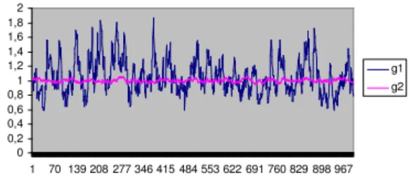
a) the stochastic productivity variables,g1tandg2t;
b) the aggregate technology growth rate;
c) the share of researchers engaged in scientific/technological activity 1,n1t;
d) the aggregate consumption growth rate.
The main feature of the results for the referred aggregates is that they change substantially each time the example is run. As stated in previous sections, the fact that any of the two projects can perform better in each moment of time implies that it is not known in anticipation which is the project that will attract more researchers; since the rule to change research strategies is an adaptive rule, the time trajectories can follow substantially different paths for the same parameters and initial values of variables.
In appendix B we present several time paths, for the previously mentioned variables. The first set of figures (figures 1 to 3) is a set of three possible realizations of the productivity variables(g1tandg2t) trajectories over time. As we expected, the two series alternate over time as the best result regarding research productivity. The main regularity is the one imposed by the heterogeneity source: the first
series presents a well evident higher volatility. The seriesg2displays a lower research risk, but, as
assumed, the two series present an equal expected outcome: E(g1) = E(g2) = 1. The two time
trajectories have differences for each one of the examples, given the stochastic component governing the Markov process. Nevertheless, there is a pattern: the higher volatility regarding the first research project, the same expected value, the reversion to the mean characteristic and the variability relating to the strategy that best performs are features present in any of the three first figures.
the property of decreasing marginal returns, the long run value of this rate is, in the absence of random
productivity, equal to zero. As displayed, the growth rate ofAt fluctuates around a constant value.
The important evidence is that there is not an identifiable pattern of evolution in time for this variable. The bounded rationality setup contributes to periods of high and low volatility to coexist in a perfectly unpredictable way. The only element in common among the lines in figures 4 to 6 is the zero expected value.
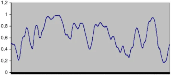
We now turn to the graphical representation of the share of researchers affected to each of the two R&D projects. Figures 7 to 9 display the share of individuals working in knowledge creation that are associated with type 1 activities (symmetric lines would represent the share of individuals engaged in type 2 research activities). The adaptive learning process and the constant change in terms of the best performing strategy are the two key points explaining the absence of a pattern linking the three time paths in consideration. A same set of parameters gives place to a potentially infinite number of solutions for the time trajectory ofnt; furthermore, since there is not a productivity value that assumes itself as the best one for a long period of time, the variable under appreciation does not tend to stay near zero or near one for long periods of time, meaning this that one of the projects does not tend to concentrate all the researchers, and consequently researchers mobility is a frequent feature in our economic setup.
The growth rate of consumption is, in our model, the one in expression (15). We verify that this
growth rate is a function of At and of a set of parameters. In this way, the behavior over time of
the growth rate of ctis qualitatively the same behavior of the technology aggregate variable. We
have mentioned that Athas an expected constant long run value and thus the expected long run
value of the consumption growth rate is also constant. From (16) is true thatA¯ =hEω(g)i1/(1
−φ) =
1 25×0.06
1/(1−0.25)
= 0.582(note in this expression that the expected productivity value is divided
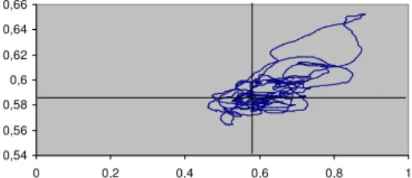
by 25, according to the calibration aspect referred in the beginning of the section). The expected long run value of consumption growth isc¯= 201.[1×0.582−(0.04−0.01)] = 0.0266. The consumption growth rate deviates from the average value in all the three presented figures [figures 10 to 12] but there is no regular pattern regarding the moments in which such deviations are more pronounced. The main feature is once more the absence of a predictable pattern. In this way, we have proposed an explanation to consumption growth unpredictability based on different degrees of uncertainty of the R&D activities. Two more items are subject to graphical representation in appendix B. These two items allow for a clearer picture about the unpredictability properties of our model. The first set of drawings [figures 13 to 15] relates to the graphical representation ofA2(in the vertical axis) relatively toA1(in the horizontal axis). The second set [figures 16 to 18] is the set of stable trajectories between the consumption-capital ratio and each one of the two technology variables, according to the saddle-path expression derived in appendix A, (22).
Figures 13 to 15 represent the level of technology in research sector 2 for each level of technology in research sector 1. The two lines that cross the graphic correspond to the expected steady state values
¯
A1 = ¯A2 =0.582. The steady state point is the one in the intersection of the two lines. Volatility
implies that there is not a unique equilibrium value but a large set of values that accumulate around the mentioned point. Confirming the information of the previous figures, larger deviations occur in the direction of higher technology values, and relatively high values for one technology variable tend to be accompanied by relatively high values of the other variable. The different shape of the line for each one of the three examples is evident in the figures.
Finally, figures 16 to 18 are saddle-path trajectories that obey equation (22) in appendix A. These
tra-jectories indicate how the consumption-capital ratio, denoted byψt, converges to the expected steady
values is the reason for the difference in shape between the two time trajectories. These trajectories have positive slopes [according to (22)] but they are not straight lines; they are collections of points that gravitate around the steady state but where it is identifiable a tendency for a positive relation between variables: relatively high values of the technology variables imply, generally speaking, a tendency for
ψthigher values. Saddle-paths have different shapes but similar qualitative properties for simulations
with a same set of parameters.
5. DISCUSSION – HETEROGENEOUS RESEARCHERS AND ENDOGENOUS FLUCTUATIONS
The present study intends to give an explanation about why macroeconomic time series display a not completely predictable pattern over time. Although this is a partial analysis, since it considers only one source of endogenous fluctuations (a bounded rationality mechanism linked to the R&D investors decisions), it is sufficiently relevant to produce the kind of business cycles that we encounter in reality. Therefore, our most important argument goes beyond the simple heterogeneity of research projects; the argument is that differences in the way economic agents in some sector of activity conduct their businesses and take autonomous decisions may have widespread implications over the main economic aggregates time series, producing everlasting fluctuations where, in conventional models with fully rational agents, we would certainly find a steady long term behavior.
Traditionally in economic literature economic fluctuations can be interpreted relying on two strands of thought. One is the Keynesian view that output and other real aggregate variables move according to monetary and other aggregate demand disturbances, given the evidence of a sluggish adjustment in nominal prices and wages. The second interpretation is the one developed by Kydland and Prescott (1982), Long and Plosser (1983), Christiano and Eichenbaum (1992) and Baxter and King (1993), among many others, which has received the designation of real business cycle (RBC) theory. Our explanation of fluctuations ignores any monetary phenomenon and thus it has an RBC flavour. Indeed, it is through the consideration of a random component linked to technology generation that fluctuations arise.
Nevertheless, there is a substantial difference between the presentation in the previous sections and RBC models. This distinction relates to: (1) there are no technological shocks; one just considers that different R&D projects have different degrees of risk; (2) fluctuations are the direct result of absence of full rationality. Instead of considering that short run variations in aggregate output and consumption are the consequence of disturbances in technology (or other variables, like government purchases), we disaggregate the research activity in a large number of research projects and we take a simple but intuitive distinction between projects – the degree of uncertainty attached to R&D projects varies, even for projects with a same expected return. The second feature, the bounded rationality setup, completes our fluctuation mechanism: if the researchers were capable of changing projects every time they found a better opportunity to make their activity more profitable, long term productivity time paths would be smooth and, given the link that our model establishes between this and other real variables like consumption, no cycles would be observable. But real life does not allow for such a perfect behavior. Researchers have different skills, and therefore the mobility of individuals between projects is reduced; many times contract obligations do not allow for a project to be abandoned at the date that it is desirable for the researcher to do so; the researcher does not have, in most circumstances, the sufficient knowledge / information about the outcome of other R&D activities.
In the light of the arguments just presented we can frame our model in the following way: the heterogeneous researchers model is an RBC model in the sense that,
(a) the basic setup corresponds to an aggregate economic growth model (and growth and fluctua-tions are not different phenomena that can be studied independently from each other);
(b) fluctuations are (can be) the result of nondeterministic technology progress;
(d) without the stochastic component, the economy would not display long term fluctuations. and it adds two new features to such an interpretation of aggregate behavior; namely,
(e) heterogeneity of research activity;
(f) bounded rationality in research.
These two features allow for an RBC model where cycles are not the result of exogenous random shocks but the result of the intrinsic random nature of purposive R&D, which is a more reasonable source of explanation for aggregate observed behavior in modern economies, where R&D is the result of highly planned activities rather than something that happens from time to time as a consequence of what some brilliant mind is capable of conceiving.
Two important issues remain to be addressed in this discussion. The first relates to the nature of fluctuations: should these be considered as the result of deterministic or stochastic sources? The second is linked to the relation between the model’s results and empirical evidence. Namely, we have used the technological heterogeneity to illustrate consumption long term patterns of evolution; are these the patterns that we observe in the real world?
In the heterogeneous researchers model, randomness is present. But it is not solely randomness that produces the kind of observed aggregate behavior. As Gomes (2005) explains, two elements are
essential to produce unpredictable long run fluctuations in an adaptive learning context: (i) a bounded
rationality mechanism; (ii) the individual time series must reflect a situation under which one of the
outcomes is not systematically better or worse than the others. Therefore, randomness in productivity is important, but without bounded rationality and alternate best performances, the aggregate time series of consumption (and output) would just look like the path relating to the individual productivity variables. Despite the fact that our fluctuations are not just the result of randomness and that chaotic features are introduced through the rationality mechanism that is adopted, no strange dynamics would be produced, under our setup, without such random component. In this way, our model allows for an intermediate answer in what concerns the recent discussion about the nature of aggregate fluctuations. Contemporary literature on aggregate fluctuations emphasizes that these can be produced without the need for random variables. Assuming increasing returns and an open economy [Aloi et al. (2000)], exter-nalities in production [Christiano and Harrison (1999)], or credit constraints [Caballé et al. (2004)], many authors are today able of replicating economic conditions under which aggregate variables behave in such a way that their time paths are impossible to predict, and this assuming deterministic scenarios. Cyclical and chaotic equilibria are systematically found in the cited studies for reasonable values of parameters.
As Bullard and Butler (1991) state: “Nonlinear dynamic models (. . . ) offer the possibility of ex-plaining economic phenomena in a purely endogenous manner, without resorting to ad hoc stochastic specifications.” (page 8). The questions we may ask are whether, on one hand, should we look at aggregate data as produced only by deterministic factors? and, on the other hand, are stochastic spec-ifications necessarily ad hoc? To the first question, the literature has developed a significant set of tentative answers. One of the most important is the strand of analysis that was initiated by Barnett and Chen (1988), who have proposed to test economic data in search for chaos. Finding chaos in eco-nomic time series would mean that fluctuations are indeed endogenous and that random variables are not important determinants of aggregate behavior. Although a consensus has not been produced so far, the large majority of studies in this field [e.g. Shintani and Linton (2003) and Serletis and Shintani (2003)] finds statistical results that cast relevant doubt over the usefulness of understanding economic data as chaotic.
that the model proposed in this paper gives a possible logical answer: the outcome of R&D projects is unpredictable by nature, and it is the different degree of uncertainty of each project that triggers the economic behavior under which aggregate variables (in the case, consumption) display a chaotic kind of evolution over time.3
A last subject of discussion relates to the reasonability of the found consumption time series. Are these coherent with observed data and with economic interpretations of aggregate consumption be-havior? Note the following features of our consumption results: (i) there is persistence over time, that is, the variability of consumption growth is low when compared with the variability of the aggregate
technology variable; (ii) the consumption growth rate does not depart significantly from its expected
value (changes in the consumption growth rate do not go beyond two percent points for the analyzed period, which includes the first thousand observations).
The relative constancy of consumption growth is characterized by Reis (2005), who, noting a well documented evidence, states that “one of the stylized facts about economic growth in the United States in the past century is that consumption, like income, has grown at an approximately con-stant rate.” (page 5). European countries and developing economies also display relative consumption growth smoothness (when compared to other aggregate time series, like the ones relating technological progress; an observation of some OECD and IMF statistical data confirms this immediately).
In what concerns the coexistence of unpredictable periods of relatively high with relatively low consumption growth, note that this is a direct result of the way consumption growth is dependent on technological progress in our model. Nevertheless, there is theoretical reasoning that supports evidence at this level. For instance, Parker and Preston (2004) emphasize precautionary saving as a source of unpredictability in consumption – because people save to consume in the future, we may even observe countercyclical movements in expected consumption growth. In other analysis, Sommer (2003) explores the role of habit formation; habit formation means that consumers become addicted to the level of consumption they experienced in the past, and thus some persistence must be observed in consumption growth paths. In our results this persistence is present; high and low consumption growth rates are, alternatively, maintained over a few periods of time, independently of the technology index growth variability over time.
6. CONCLUSIONS
In an economy there are many types of R&D activities. Some have a certain degree of certainty relating expected outcomes; others involve a considerable degree of risk: results may be the expected ones, much better than expected or, in opposition, much worse. Having this observation in mind, we have developed an optimal control problem for a representative consumer and a two-sector setup. The two assumed economic sectors were a final goods sector and a technological sector. The technological sector had the peculiarity of disaggregating research projects in a way that different uncertainty degrees in R&D projects were highlighted.
Combining the existence of distinct opportunities regarding innovation strategies with a rule of bounded rationality behavior for the agents engaged in the technology production process, we have attempted to put together an explanation for aggregate consumption growth paths volatility and un-predictability. It was shown that a same set of parameters and initial values of variables gives place to different consumption growth trajectories each time the example is concretized.
3By now the notion of chaos needs a clarification. If one wants to be rigorous, our long run result concerning the consumption
The developed model can be associated to the real business cycle literature, in the sense that it relies on technology stochasticity to explain real economic aggregates fluctuations (with a complete absence of nominal variables). The model’s marginal contribution is that it allows for a result of compromise - endogenous fluctuations do not come exclusively from deterministic sources, but the source of ran-domness has economic meaning: R&D projects have different degrees of associated uncertainty, and researchers tend to be dispersed along these projects.
Bibliography
Aloi, M., Dixon, H., & Lloyd-Braga, T. (2000). Endogenous fluctuations in an open economy with
increas-ing returns to scale. Journal of Economic Dynamics and Control, 24:97–125.
Anderson, S., De Palma, A., & Thisse, J. (1992). Discrete choice theory of product differentiation. MIT Press.
Arrow, K. & Kurz, M. (1970). Public investment, the rate of return, and optimal Fiscal policy.
Azariadis, C. & Kaas, L. (2002). Asset Price Fluctuations without Aggregate Shocks. Technical report, University of California and University of Vienna.
Barnett, W. & Chen, P. (1988). The Aggregation-Theoretic Monetary Aggregates are Chaotic and Have Strange Attractors: An Econometric Application of Mathematical Chaos. In W. A. Barnett, E. B. &
White, H., editors,Dynamic Econometric Modeling, pages 199–246. Cambridge University Press.
Barucci, E. (1999). Heterogeneous Beliefs and Learning in Forward Looking Economic Models.Journal of
Evolutionary Economics, 9(4):453–464.
Baxter, M. & King, R. (1993). Fiscal Policy in General Equilibrium. The American Economic Review,
83(3):315–334.
Becker, R. & Tsyganov, E. (2002). Ramsey Equilibrium in a Two-Sector Model with Heterogeneous
House-holds. Journal of Economic Theory, 105(1):188–225.
Brock, W. & Hommes, C. (1997). A Rational Route to Randomness. Econometrica, 65(5):1059–1095.
Brock, W. & Hommes, C. (1998). Heterogeneous Beliefs and Routes to Chaos in a Simple Asset Pricing
Model. Journal of Economic Dynamics and Control, 22(8):1235–1274.
Brock, W., Hommes, C., & Wagener, F. (2001). Evolutionary Dynamics in Markets with Many Trader Types. Technical report, CeNDEF, Amsterdam.
Bullard, J. & Butler, A. (1991). Nonlinearity and Chaos in Economic Models: Implications for Policy Decisions. Technical Report 1991-002B, Federal Reserve Bank of St. Louis.
Caballé, J., Jarque, X., & Michetti, E. (2004). Chaotic Dynamics in Credit Constrained Emerging
Economies. Technical Report 121, Barcelona Economics.
Chiarella, C. & He, X. (2002). An Adaptive Model on Asset Pricing and Wealth Dynamics with Heteroge-neous Trading Strategies. Technical report, University of Technology.
Christiano, L. & Eichenbaum, M. (1992). Current Real Business Cycle Theories and Aggregate Labor
Market Fluctuations. American Economic Review, 82:430–450.
Christiano, L. & Harrison, S. (1999). Chaos, Sunspots and Automatic Stabilizers. Journal of Monetary
De Grauwe, P. & Grimaldi, M. (2002). The Exchange Rate and its Fundamentals: a Chaotic Perspective. Technical Report 639, CESifo.
Evans, G. W. & Honkapohja, S. (2001).Learning and Expectations in Macroeconomics. Princeton University Press.
Gaunersdorfer, A., Hommes, C., & Wagener, F. (2003). Bifurcation Routes to Volatility Clustering under Evolutionary Learning. Technical report, CeNDEF, Amsterdam.
Gomes, O. (2005). Volatility, Heterogeneous Agents and Chaos. The Electronic Journal of Evolutionary
Modeling and Economic Dynamics, 3(1047):1–32.
Hommes, C. H., Sonnemans, J., Tuinstra, J., & van de Velden, H. (2002). Expectations and Bubbles in Asset Pricing Experiments. Technical Report 02-05, CeNDEF, University of Amsterdam.
Jones, C. I. (1995). R & D-Based Models of Economic Growth.Journal of Political Economy, 103(4):759–784.
Jones, C. I. (2003). Population and Ideas: A Theory of Endogenous Growth. In Aghion, P., Frydman, R., Stiglitz, J., & Woodford, M., editors,Knowledge, Information, and Expectations in Modern Macroe-conomics, pages 498–521, Princeton, New Jersey. Princeton University Press. Honor to Edmund S. Phelps.
Kurz, M. (1997a). Asset prices with rational beliefs. In Kurz, M., editor,Endogenous Economic Fluctuations: Studies in the Theory of Rational Belief, number 6 in Springer series in Economic Theory, chapter 9. Springer.
Kurz, M. (1997b). Asset Prices with Rational Beliefs. In Kurz, M., editor,Endogenous Economic
Fluctua-tions: Studies in the Theory of Rational Belief, number 6 in Studies in Economic Theory, chapter 7, pages 211–250. Springer-Verlag, Berlin and New York.
Kurz, M. & Beltratti, A. (1997). The Equity Premium is no Puzzle. In Kurz, M., editor, Endogenous
Economic Fluctuations: Studies in the Theory of Rational Belief, number 6 in Studies in Economic Theory, chapter 11, pages 283–316. Springer.
Kurz, M., Jin, H., & Motolese, M. (2003). Endogenous Fluctuations and the Role of Monetary Policy. In Aghion, P., Frydman, R., Stiglitz, J., & Woodford, M., editors,Knowledge, Information, and Expectations in Modern Macroeconomics (in Honor of Edmund S. Phelps), pages 188–227. Princeton University Press, Princeton, New Jersey.
Kurz, M. & Motolese, M. (2001). Endogenous uncertainty and market volatility. Economic Theory,
17(3):497–544.
Kurz, M. & Schneider, M. (1996). Coordination and correlation in Markov rational belief equilibria.
Economic Theory, 8(3):489–520.
Kydland, F. & Prescott, E. C. (1982). Time to Build and Aggregate Fluctuations.Econometrica, 50(6):1345– 1370.
Long, J. B. & Plosser, C. I. (1983). Real Business Cycles. Journal of Political Economy, 91(1):39–69.
Lorenz, H.-W. (1997).Nonlinear dynamical economics and chaotic motion. Springer-Verlag, Berlin and New
York, 2 edition.
Maliar, L. & Maliar, S. (2001). Heterogeneity in Capital and Skills in a Neoclassical Stochastic Growth
Manski, C. & McFadden, D. (1981). Structural analysis of discrete data with econometric applications. MIT Press, Cambridge, Mass.
Negroni, G. (2003). Adaptive Expectations Coordination in an Economy with Heterogeneous Agents.
Journal of Economic Dynamics and Control, 28:117–140.
Nourry, C. & Venditti, A. (2001). Determinacy of equilibrium in an overlapping generations model with
heterogeneous agents.Journal of Economic Theory, 96:230–255.
Parker, J. A. & Preston, B. (2004). Precautionary Saving and Consumption Fluctuations. Technical report, Princeton University and Columbia University.
Rebelo, S. (1991). Long-Run Policy Analysis and Long-Run Growth. Journal of Political Economy, 99:500–
521.
Reis, R. (2005). The Time-Series Properties of Aggregate Consumption: Implications for the Costs of Fluctuation. Technical report, Princeton University.
Romer, P. (1990). Endogenous Technological Change. Journal of Political Economy, 98:S71–S102.
Romer, P. M. (1986). Increasing Returns and Long-Run Growth. The Journal of Political Economy,
94(5):1002–1037.
Sargent, T. J. (1993).Bounded rationality in macroeconomics. Clarendon Press, Oxford.
Serletis, A. & Shintani, M. (2003). No evidence of chaos but some evidence of dependence in the U.S. stock market. Chaos, Solitons and Fractals, 17(2):449–454.
Shintani, M. & Linton, O. (2003). Is There Chaos in The World Economy? A Nonparametric Test Using
Consistent Standard Errors*.International Economic Review, 44(1):331–358.
Sommer, M. (2003). Habits, Sentiment and Predictable Income in the Dynamics of Aggregate Consump-tion. International Monetary Fund.
Tuinstra, J. & Wagener, F. O. O. (2003). On Learning Equilibria. Technical report, CeNDEF, Amsterdam.
A. PROOF OF PROPOSITIONS
Proof of proposition 1. The Arrow and Kurz (1970) theorem may be applied to our optimal control prob-lem as follows:
“Define ℵ0(k
t, Aht), h = 1, ..., H to be the maximum of ℵ(kt, Aht, ct), with respect to ct. If
ℵ0(k
t, Aht)is concave inkt andAht, for givenpkt andpAht, then the necessary conditions (10) to (13) are also sufficient.”
Condition (10) allows to write function (17).
ℵ0(k
t, Aht) =
U(p−kt1/θ) +pkt. h
At.f(kt)−p
−1/θ
kt −δ.kt
i +
H P
h=1
pAht.ght.fA(At)−ω.Aht
(17)
We want to averiguate ifℵ0is a concave function. It is concave if the correspondent Hessian matrix is
matrix of the form,
H(ℵ0) =
∂2ℵ0
∂k2
t
∂2ℵ0
∂k.
t∂A1t · · ·
∂2ℵ0
∂k. t∂AHt
∂2ℵ0
∂A1t.∂kt
∂2ℵ0
∂A2
1t · · ·
∂2ℵ0
∂A1t∂AHt
..
. ... . .. ...
∂2ℵ0
∂AHt.∂kt
∂2ℵ0
∂AHt∂A1t · · ·
∂2ℵ0
∂A2 Ht
Proceeding with the computation of the matrix elements, one gets,
H(ℵ0) =
0 ζ.pkt.n1t · · · ζ.pkt.nHt
ζ.pkt.n1t −ξ.pA1t.g1t.n21t · · · −ξ.pA1t.g1t.n.1tnHt ..
. ... . .. ...
ζ.pkt.nHt −ξ.pAHt.gHt.n.Htn1t · · · −ξ.pAHt.gHt.n2Ht ,
withξ≡φ.(1−φ).A−t(2−φ).
(18)
To find out if (18) is a negative semidefinite matrix, we take the correspondent definition: a(H+ 1)×
(H+ 1)matrix is classified as negative semidefinite if for all vectorsz= [z0 z1. . . zH]∈RH+1, the conditionzT.H(ℵ0).z≤ 0is satisfied. The condition is verified for combinations of parameters and variables that make (14) true. Therefore, necessary conditions are not universally sufficient; they are
sufficient under condition (14).
Proof of proposition 2. Consider the set of equations (4). Because there is decreasing marginal returns in the production of technology, the technology variables will tend to long run constant values, and thus
∆Aht= 0defines a steady state with a constantA¯value. Furthermore, because, under definition (2),
E(gt+1) = E(gt)λ, one observes thatE¯(g) = 1defines the same steady state point, for every R&D
project. As a consequence, to determine the long run expected value ofAt, we substitute in (4)ghtby
1. Therefore,∆Aht= 0⇒A¯h=ω
−1/(1−φ)
, ∀h, andA¯= ¯Ah.
As regarded, there is a unique steady state level for technology. In what concerns consumption and capital variables, expression (15) indicates that consumption grows at a constant rate in the steady
state, given the constant value ofA¯. Relatively to capital, equation (2) implies that consumption and
capital must grow at a same steady state rate, and thus a variableψt=ct/ktwill grow at a constant
long run growth rate. The equation that reflects the time evolution of this variable is
∆ψt=
ψt−
ζ+1
θ
.At−
θ−1
θ .δ−
1
θ.ρ
.ψt (19)
The unique steady state value of the consumption-capital ratio is∆ψt= 0⇒ψ¯= ωζ1/+1(1/θ−φ)+ θ−1
θ .δ+
1 θ.ρ.
The pair( ¯A,ψ¯)is the unique steady state point of the system.
Proof of proposition 3. Saddle-path stability implies a Jacobian matrix with some (but not all) eigenval-ues in the interval(−2,0), since the system is defined in terms of first differences. Considering the
and (19), in the vicinity of the steady state. Note that the matrix in the system is the Jacobian matrix.
∆ψt
∆A1t
∆A2t .. .
∆AHt = ¯
ψ −(ζ+ 1/θ).n1.ψ¯ −(ζ+ 1/θ).n2.ψ¯ · · · −(ζ+ 1/θ).nH.ψ¯
0 −(1−φ.n1).ω φ.n2.ω · · · φ.nH.ω
0 φ.n1.ω −(1−φ.n2).ω · · · φ.nH.ω ..
. ... ... . .. ...
0 φ.n1.ω φ.n2.ω · · · −(1−φ.nH).ω .
ψt−ψ¯
A1t−A¯
A2t−A¯ .. .
AHt−A¯ (20)
The Jacobian matrix in (20) is a(H+ 1)×(H+ 1)squared matrix with trace=ψ¯−ω.(H−φ)and
determinant= ¯ψ.(−ω)−1.(1−φ). Computing eigenvalues, these areη
1= ¯ψ >0, η2=−ω.(1−φ)< 0 andη3 = . . . = ηH+1 = −ω < 0. As a result, there is one positive eigenvalue corresponding to
the one-dimensional unstable arm of the system andHnegative eigenvalues (that are smaller than 1
in absolute value), and thus the stable trajectory has dimensionH. Because there are simultaneously
stable and unstable trajectories, the equilibrium is defined by saddle-path stability.
Proof of proposition 4. Each one of the negative eigenvaluesη2toηH+1has an associated eigenvector.
TheseHeigenvalues compose a matrix from which we can derive the slope of the stable trajectory. For
η3=. . .=ηH+1=−ωthe eigenvectors arePi= 0 −nnH1 −
nH
n2 · · · 1
/
,i= 3, . . . , H+ 1;
for η2 we have the following eigenvector: P2 =
h (θ−1).ψ¯
θ.[ψ¯+ω.(1−φ)] 1 1 · · · 1
i/
. The matrix
P =
P2 P3 · · · PH+1 is a(H+ 1)×H matrix that can be divided in two; the slope of the stable trajectory is given by -π.Π−1, whereπis the first line ofPandΠ is the square matrix composed
by the lines 2 toH+ 1ofP. Some computation leads to a vector
n1 n2 · · · nH as the first line ofΠ−1. This is the only line of the matrix that one needs to calculate the slope results, because only the first element ofπis different from zero. We have then,
Slope of the stable trajectory= θ−1
θ .
¯
ψ
¯
ψ+ω.(1−φ).
n1 n2 · · · nH (21)
The slope of the stable trajectory is a set of positive values, given the constraints over parameter values that were established. Therefore, the stable trajectory is defined as
ψt−ψ¯=
θ−1
θ .
¯
ψ
¯
ψ+ω.(1−φ).
n1.(A1t−A¯) +n2.(A2t−A¯) +. . .+nH.(AHt−A¯) (22)
From (22) it is understandable that a convergence to the steady state through increasing values of technology levels implies that the consumption-capital ratio will also exhibit an increasing behavior. This result is common to this kind of models and it is obvious and intuitive: a higher technology level means that a final good can be produced with lower quantities of capital and thus a higher share of produced final goods can be directed to consumption. Note that (22) is equivalent to (23), given the definition of aggregate technology level,
ψt= ¯ψ−
θ−1
θ .
¯
ψ
¯
ψ+ω.(1−φ).A¯+
θ−1
θ .
¯
ψ
¯
ψ+ω.(1−φ).At (23) Result (23) would be the one obtained directly if we had constructed the linearized model for the system
Orlando Gomes
B. NUMERICAL EXAMPLE TIME TRAJECTORIES
0 0,5 1 1,5 2 2,5
1 68 135 202 269 336 403 470 537 604 671 738 805 872 939 g1
g2
Figure 1 – Productivity variables time paths (example 1)
0 0,2 0,4 0,6 0,8 1 1,2 1,4 1,6 1,8 2
1 70 139 208 277 346 415 484 553 622 691 760 829 898 967 g1 g2
Figure 2 –Productivity variables time paths (example 2)
0 0,5 1 1,5 2 2,5
1 71 141 211 281 351 421 491 561 631 701 771 841 911 981 g1
g2
Figure 3 – Productivity variables time paths (example 3)
-0,04 -0,03 -0,02 -0,01 0 0,01 0,02 0,03 0,04 0,05 0,06
Figure 4 –A growth rate (example 1)
-0,03 -0,02 -0,01 0 0,01 0,02 0,03 0,04
Figure 5 –A growth rate (example 2)
-0,03 -0,02 -0,01 0 0,01 0,02 0,03 0,04 0,05
Heterogeneous Researchers in a Two-Sector Representative Consumer Economy
0 0,2 0,4 0,6 0,8 1 1,2
1 59 117 175 233 291 349 407 465 523 581 639 697 755 813 871 929 987
Figure 7 –n1 (example 1)
0 0,2 0,4 0,6 0,8 1 1,2
1 59 117 175 233 291 349 407 465 523 581 639 697 755 813 871 929 987
Figure 8 –n1 (example 2)
0 0,2 0,4 0,6 0,8 1 1,2
1 59 117 175 233 291 349 407 465 523 581 639 697 755 813 871 929 987
Figure 9 –n1 (example 3)
0 0,005 0,01 0,015 0,02 0,025 0,03 0,035 0,04 0,045 0,05
1 61 121 181 241 301 361 421 481 541 601 661 721 781 841 901 961
Figure 10 –c growth rate (example 1)
0 0,005 0,01 0,015 0,02 0,025 0,03 0,035 0,04 0,045
1 61 121 181 241 301 361 421 481 541 601 661 721 781 841 901 961
Figure 11 –c growth rate (example 2)
0 0,005 0,01 0,015 0,02 0,025 0,03 0,035 0,04 0,045 0,05
1 61 121 181 241 301 361 421 481 541 601 661 721 781 841 901 961
Orlando Gomes
0,56 0,57 0,58 0,59 0,6 0,61 0,62 0,63 0,64 0,65 0,66
0 0,2 0,4 0,6 0,8 1 1,2
Figure 13 –Relation between technology lev-els (example 1)
0,54 0,56 0,58 0,6 0,62 0,64 0,66
0 0,2 0,4 0,6 0,8 1
Figure 14 –Relation between technology lev-els (example 2)
0,56 0,57 0,58 0,59 0,6 0,61 0,62 0,63 0,64 0,65 0,66
0 0,2 0,4 0,6 0,8 1
Figure 15 –Relation between technology lev-els (example 3)
0,4 0,45 0,5 0,55 0,6 0,65 0,7 0,75 0,8 0,85 0,9
0,4 0,5 0,6 0,7 0,8 0,9 1
Figure 16 –Stable trajectories (consumption-capital ratio /A1,A2) (example 1)
0,4 0,45 0,5 0,55 0,6 0,65 0,7 0,75 0,8 0,85
0,4 0,5 0,6 0,7 0,8 0,9 1
Figure 17 –Stable trajectories (consumption-capital ratio /A1,A2) (example 2)
0,4 0,45 0,5 0,55 0,6 0,65 0,7 0,75 0,8 0,85 0,9
0,4 0,5 0,6 0,7 0,8 0,9 1