Herding and Positive Feedback Trading in the
Portuguese Stock Exchange: An Exploratory
Investigation
by Vasileios Kallinterakis
1and Mario Pedro Leite Ferreira
2Abstract
The heterogeneity inherent in the composition of the investors’ population is a factor conducive to the complexity of the market. Heterogeneous backgrounds are expected to lead to divergence in investors’ decision-making. However, evidence suggests that the temporary convergence of beliefs and actions is a possibility. Our research attempts to address two aspects of this convergence, namely positive feedback trading (“trend-chasing”) and herding. Using data from the Portuguese PSI-20 market index, we test for herding and positive feedback trading for the period since the inception of the index (January 1993). In line with Hwang and Salmon (2004), herding appears to be rising during periods of “definitive” market direction and exhibits descending tendencies during periods of market fluctuations. Results indicate the significance of herding and positive feedback trading towards the index, both of which appear to be experiencing a sharp rise between 1996 and 1999. This coincides with the Portuguese market’s “boom-bust” in the second half of the 1990’s.
1Durham Business School, Department of Economics and Finance, Durham University, 23/26 Old
Elvet, Durham DH1 3HY, Tel: +44 (0)191 334 6340, Fax: +44 (0)191 334 6341
Corresponding author: Email: vasileios.kallinterakis@durham.ac.uk.
2 Universidade Católica Portuguesa, Centro Regional do Porto, Rua Diogo Botelho, 1327,
I. Introduction
Securities’ investors constitute a rather heterogeneous group as they may differ in terms of educational background, investment experience, information processing and capital resources. As a result, their population can be characterized by a certain element of heterogeneity, which has the potential of manifesting itself in their investment decisions. Traders may follow a line of strategy today and, contingent upon its success, may continue to pursue it, adapt it or discard it. This notion of “competitive” strategies in the marketplace has been advocated in particular by behavioural (Hirshleifer, 2001) and adaptive Finance proponents (Arthur, 1994; Arthur, 1997; Arthur, 1999; Arthur, 2000a; Arthur, 2000b; Farmer, 2001; Farmer, 2002: Farmer and Lo, 1999; Mauboussin, 2002).
In such a heterogeneous setting, we would expect traders to normally differ in their trading patterns, i.e. exhibit divergence. It might be the case, however, that divergence is not the case and that it is convergence that finally prevails. Two of the most cited forms of such convergence in the Finance literature are positive feedback trading and herding, both of which relate to the potential co-directional behaviour of investors.
Positive feedback trading relates to the practice of following past price patterns (De Long, Shleifer, Summers and Waldman, 1990). Herding, on the other hand, pertains to collective behavioural phenomena, where people imitate the decisions of others (Devenow and Welch, 1996). A positive feedback trader, trades towards the direction suggested by historical prices, while a person who herds follows the actions of others. These behavioural patterns bear interesting implications for market prices, as they may well lead to trend-chasing phenomena (Bikhchandani and Sharma, 2001) with the potential for mispricing (Hirshleifer, 2001) and excess volatility (Koutmos and Saidi, 2001).
We test for herding and positive feedback trading on the basis of aggregate data for the Portuguese stock exchange employing two models, one for feedback trading, and the other for herding. The choice of Portugal was motivated by the fact that, although previous research (Lobao and Serra, 2002) addressed the issue of herding at the micro-level (using equity funds’ accounts), herding has not been investigated in that market using aggregate data (such as returns). Our work also contributes to
existing Finance research, as the joint behaviour of herding and positive feedback trading on the basis of aggregate data has received little attention, even though they constitute very affiliate concepts.
The rest of the paper is structured as follows: Section II includes an overview of the notions of herding and positive feedback trading, while Section III includes a brief overview of the Portuguese market’s contemporary evolution. Section IV discusses the data used in this research and delineates the methodology utilized. Section V presents and discusses the results and Section VI concludes.
I. Theoretical Background II. a. Positive Feedback trading
In the stock-trading context, feedback trading has been used as a term to describe the conduct of a specific type of trader whose investment decisions are a function of historical prices. If he trades in the same direction with past prices he is called “positive feedback trader”, while if he trades in the opposite direction, he is called “negative feedback (contrarian) trader”.
A number of psychological biases can be associated with positive feedback trading. Positive feedback trading can, for example, be reinforced through the representativeness heuristic (overweighting recent data as representative of a trend-at-works) and the conservatism bias (underweighting recent data if the perception of an opposite trend-at-works prevails), (Barberis, Shleifer and Vishny, 1998). It can also be fuelled by the overconfidence-bias (aggressive trading following a “euphoric” period of recent gains (Odean, 1998; Glaeser and Weber, 2004a; Glaeser and Weber, 2004b).
Positive feedback trading can further be motivated through the availability-heuristic. Historical data on prices, for example, are easy to find in the financial press (Huddart, Lang and Yetman, 2002), while more sophisticated data are harder to find. The simplified analysis of such data (as carried out mostly by technical analysts in the press) facilitates the communication of these “technical heuristics” to a wider audience, which is perhaps not typified by a sufficient educational background or investment experience.
Positive feedback trading, however, is not restricted to “noise” traders who may be susceptible to behavioural biases, maintain less abilities/resources or use technical analysis. A series of papers (Koutmos, 1997; Antoniou, Koutmos and Pericli, 2005) have argued that rational traders may employ trading rules based on historical prices if they feel they have to shield themselves against (or take advantage of) abrupt market movements; portfolio insurance and stop-loss orders (Osler, 2002)) are relevant here. Such strategic choices on behalf of rational traders are founded upon the belief that noise traders might push prices away from their fundamental value, thus leading to a mispricing of indefinite duration and magnitude (Barberis and Thaler, 2002). De Long et al. (1990), Farmer (2002), Farmer and Joshi (2002) and Andergassen (2003) discuss the possibility of rational speculators actually riding on the waves of the positive feedback trading in order to take advantage of the perceived mispricing induced by noise traders.
II. b. Herding
Herding, as Hirshleifer and Teoh (2003) have noted, involves a “similarity in behaviour” following “interactive observation”. Therefore, herding is witnessed when people follow the observable information, actions or the payoffs from the actions of others.
In line with popular beliefs, the impetus underlying imitation has been assumed to lie within the human nature: people may simply prefer to copy others. This tendency towards conformity (Hirshleifer, 2001) may well be related to the interaction of people, as they communicate with one another. Communication may be explicit (when people are conversing (Shiller, 1995), yet it may also be tacit (when people observe others’ choices, for example in fashion (Bikhchandani, Hirshleifer and Welch, 1992).
Devenow and Welch (1996) argued that following the decisions of others may be associated with informational payoffs, when one: a) possesses no private information, b) has private information, yet is uncertain about it, perhaps because it is of low quality or c) perceives others as better-informed. If so, he may choose to free-ride on the informational content of others’ actions, thus tackling the problem of information acquisition (or uncertainty). Also, if an investor possesses private information, he may still decide to ignore it and follow the actions of others, when the
information conveyed by others’ actions provides a useful set of information on its own (Bikhchandani and Sharma, 2001); the latter is expected to lead to what is known as an “informational cascade”.
Professionals, be they fund managers or analysts, are subject to periodic evaluation (Scharfstein and Stein, 1990; Lakonishok et al., 1992; De Bondt and Teh, 1997; Wermers, 1999) which is normally of a relative nature, i.e. they are evaluated against one another. Since their abilities do not exhibit uniformity, “herding” towards the perceived “benchmark” may be a viable option. Reputational reasons are also relevant here, as well-reputed professionals may decide to join the herd if the risk of failure is higher than the benefits of success by going-it-alone. Less reputed ones may also free-ride on the reputation of others by “herding” on their decisions (Truman, 1994; Graham, 1999).
However, according to Bikhchandani and Sharma (2001), a similarity of responses can also be due to commonly observed signals. Thus, changes in fundamentals becoming public knowledge have the potential of inducing people to behave in a parallel fashion, without the latter necessarily originating in irrational traits (“spurious herding”).
III. The Portuguese stock market (1977-2005)
The modern history of the stock market in Portugal can be officially traced back to early 19773. At the beginning, though, the small dimension of the market and the double-digit inflation rates led to rather limited investors’ participation. Following Portugal’s accession to the EEC in 1986, the stock market began to exhibit the first signs of euphoria. The 1986-1989 period was characterised by an increase in the number of IPO’s and the growth in trading volume. During these years, Portugal was going through a booming economic cycle sustained by the EEC accession4.
In the period between 1990 and 1993, the country’s economy enters the recession stage and the Portuguese market index displays a sharp fall. The
3 Following the 1974 coup, the stock market operations were suspended for three years. The first
session of the Portuguese stock exchange took place in Lisbon in 28/2/1977.
4 The participation in the common market and the substantial influx of European funds led to an
increase of FDI, GDP and exports. On average, the GDP grew 4.2% year to year. At the same time, inflation and unemployment decreased. In the stock exchange, growth could be observed through the following events: the first IPO in 1986, the establishment of the BVLG Index in 1988 and the first privatization in 1989.
international crisis triggered by the Gulf War, the increase of 60% in real wages and the inflation control policy were factors that deteriorated GDP-evolution and reduced investors’ confidence. According to Balbina and Martins (2002), between the end of 1989 and 1992, the market index decreased by 41.8%.
From the end of 1993 until 1998, the Portuguese stock exchange enters into a period of growth towards maturity. In the end of 1993, the Maastricht Treaty is ratified and free capital movement is regulated within the European Union, reducing investment risk in EU developing markets. In the beginning of the 1994, the Oporto and Lisbon stock exchanges merge into one single market in Lisbon. Portugal enters into a booming cycle fuelled by the US growth; FDI, exports and GDP experience a sharp growth. Privatizations, namely of blue-chip firms held by the government5, are also very intense during this period. In December 1997, the Portuguese stock exchange is upgraded by Morgan Stanley to “mature” and 19 companies are listed in the Dow Jones. Finally, in 1998, it is publicly announced that Portugal will be joining the third stage of the Monetary Union. Overall, this sequence of favourable economic events led to a substantial increase in trading activity while the market index rose by 270% (January 1996 – April 1998).
Between the end of 1998 and 2002, the Russian/Asian crises and the dotcom bubble brought about high levels of volatility to the Portuguese stock exchange. In the end of 1998, the Russian/Asian crises created instability that later spread to other developing economies, including Brazil (a preferential destination for Portuguese FDI). That instability was particularly felt in the Portuguese stock exchange between the last quarter of 1998 and the end of 1999. The decrease of the market index was clearly pointing towards a forthcoming recession.
However, in the first quarter of year 2000, there was a significant positive inversion in the market trend. This fact was mainly due to a late impact of the dotcom-bubble in Portugal (Balbina and Martins, 2002). During the last quarter of 1999 and early 2000, there was a rise in IPOs of IT-companies6 accompanied by a rally in their prices (Sousa, 2002). This rally came to an abrupt halt during the first quarter of year 2000, following the slump observed in the NASDAQ. Market stagnation became a reality until the end of 2002.
5 Examples include Brisa, Cimpor, EDP and Portugal Telecom.
After 2002, the Portuguese stock market has been attempting to recover the pre-1999 condition. To boost stock trading, the Euronext Lisbon was created in 2002. However, the market index has exhibited signs of a rather slow increase until present time. Economic recovery is still not clear in Portugal. The Euro valuation against the dollar, the slow growth of the EU and the Portuguese inability to reform the public sector are factors that condition GDP growth. Portugal did not manage to comply with the Stability and Growth Pact requirements and is now applying a restrictive policy to fight recession.
IV. a. Methodology
a) Positive feedback trading (Sentana and Wadhwani (1992))
To test for positive feedback trading, the model developed by Sentana and Wadhwani (1992) is employed here. This model has been applied for a variety of markets, both developed (Koutmos, 1997; Bohl and Reitz, 2002; Bohl and Reitz, 2003; Antoniou et al, 2005) as well as developing (Koutmos & Saidi, 2001). The model assumes two types of traders, namely “rational” ones, who maximize their expected utility and “feedback” ones, who trade on the basis of lagged past returns (one period back). The demand function for the former is as follows:
α − −
E
t 1(rt) − − − − − − − − − − − − − − − − − − − =Q
t (1) θ*(σ
2t) whereQ
t represents the fraction of the shares outstanding of the single stock (or,
alternatively, the fraction of the market portfolio) held by those traders,
E
rt t−1( ) is the expected return of period t given the information of period t-1,α
is the risk-freerate (or else, the expected return such that
Q
t= 0), ϑ is a coefficient measuring the
degree of risk-aversion and µ(
σ
2t) is the conditional variance (risk) at time t. The demand function of their feedback peers is portrayed as:Y
t =γ
1*r
t 1− (2) whereγ
1 is the feedback coefficient and
r
t 1− is the return of the previous period (t-1) expressed as the difference of the natural logarithms of prices at periods t-1 and t-2 respectively. A positive value ofγ
1 (
γ
1> 0) implies the presence of positive feedback trading, while a negative value (γ
1< 0) implies the presence of negative feedback trading (also known as “contrarian”).
In equilibrium all shares must be held, hence:
Q
t+Y
t=1(3)
E
t−1(rt) -α
If so, then: --- +γ
1*r
t−1= 1
) ( *σ
2 θ t Thus:E
rt t−1( ) – α +γ
1 *r
t 1− * ϑ * ( ) 2σ
t = ϑ * ( ) 2σ
tE
t−1(rt) = α -γ
1*r
t 1− * ϑ * (σ
t2)+ ϑ * (σ
2t) (4)which provides us with a modified version of the CAPM in the presence of feedback traders. Assuming
r
t =E
rt t−1( ) +ε
t, we have:r
t = α – (γ
1 *r
t 1− * ϑ * ( ) 2σ
t ) + ϑ * ( ) 2σ
t +ε
t (5)where
r
t represents the actual return at period t andε
t is the error term. To allow for autocorrelation due to non-synchronous trading, Sentana and Wadhwani (1992) modify (5) as follows:r
t =α
+ (φ
0 +φ
1*( ) 2σ
t )*r
t−1 + ϑ*( ) 2σ
t +ε
t (6)where
φ
0is designed to capture possible non-synchronous effects and
φ1
= - ϑ*γ
1. Thus, a negativeφ1
would indicate the presence of positive feedback trading.The addition of feedback traders in an otherwise CAPM-setting bears some interesting implications. As equation (5) shows, the inclusion of the term – (
γ
1 *r
t−1 * ϑ *(σ
t2)) leads to return autocorrelation, the magnitude of which is a function ofthe risk in the market (as denoted by(
σ
2t)). Hence, the higher the volatility grows, thehigher the autocorrelation. Also, the sign of the autocorrelation will be determined by the sign of the feedback trading prevalent among feedback traders; if positive feedback traders prevail, then the autocorrelation will be negative, whilst it will be positive in the presence of more negative feedback traders.
However, the feedback coefficient (
φ1
) is not irrelevant to volatility in this model. Positive feedback trading may well lead to the launch of a trend, thus forcing prices to fluctuate more wildly, hence becoming more volatile. The relationship can also assume a different form, as highly volatile markets may lead many investors to resort to strategies of positive feedback style (e.g. employ portfolio insurance and stop-loss orders), which might cause a general price decline (in the event of a rising trend) or further exacerbate the price slump in the case of a price fall.The implications for rational traders from a rise in volatility are also obvious. As volatility rises, so does the risk and as a result, the risk-premium required on their behalf in order to hold more shares. Assuming constant risk-aversion (the ϑ
coefficient), their ability to profit from a hypothetical trend may not be taken for granted, as the market will have grown riskier and they may well decide to liquidate their positions early on rather than follow the trend (Kyle and Wang, 1997).
In order to test for positive feedback trading on these premises, we have to specify the measurement equation for the conditional variance, as indicated by equation (6).
The conditional variance (
σ
t2) is modeled here using three differentspecifications;
2 1 2 1 2 − − + + = t t t ω β ε γσ σ
where, σt2 is the conditional variance of the returns at time t, εt is the innovation at
time t and , and are nonnegative fixed parameters.
- an EGARCH process (Nelson, 1991, Brooks, 2002): ln (
σ
t2) = ω + *β ln (σ
t2−1) + *γ (u
t 1− / (σ
t2−1) + δ *[(|u
t 1− |/ (σ
t2−1)) - (2 / π)]EGARCH allows for asymmetric responses of volatility to positive and negative shocks, since if the volatility-returns relationship is negative, γ will be negative as well. As standardized residuals from GARCH models tend to exhibit signs of leptokurtosis, we estimate the EGARCH model by assuming a Generalized Error Distribution (GED).
- A conditional variance specification relevant to the EGARCH is the Asymmetric GARCH (1,1) developed by Glosten, Jagannathan and Runkle (1993):
2 1 1 2 1 2 1 2 − − − − + + + = t t t t t ω β ε γσ δS ε σ
Here captures the asymmetric responses of volatility during positive versus negative innovations. St is a binary variable equalling one if the innovation at time t is
negative and zero otherwise. If is positive and statistically significant then negative innovations increase volatility more that positive innovations.
b) Herding (Hwang and Salmon (2004))
To test for herding, we employ the model developed by Hwang and Salmon (2004) in their study of the US and South Korean markets. This model traces its rationale back to the first herding measure proposed by Christie and Huang (1995) and Chang, Cheng and Khorana (2000) who argued that herding could be reflected in the cross-section of asset returns, in the sense that a lower (cross-sectional) dispersion of returns would indicate that assets moved in tandem with their cross-sectional mean, i.e. herded towards some sort of market consensus.
Hwang and Salmon (2004) began from parallel considerations. Instead of measuring herding using the cross-sectional deviations of returns, they tested for herding on the basis of the cross-sectional dispersion of the factor-sensitivity of assets. More specifically, they argued that when investors are driven by behavioural
biases, their perceptions of the risk-return relationship of assets may be distorted. If they do indeed herd towards the market consensus, then it is possible that as individual asset returns converge to the market return, their CAPM-betas will deviate from their equilibrium values. Thus, the beta of a stock does not remain constant (as the conventional CAPM would posit), but changes with the fluctuations of investors’ sentiment. As a result, the cross-sectional dispersion of their betas would be expected to be smaller, i.e. asset betas would tend towards the value of the market beta, namely unity. It is on these very premises that their herding measure is based.
More specifically, they assume the equilibrium7 beta (let
β
imt) and its
behaviourally biased version (
β
bimt), whose relationship is assumed to be the
following:
(
E
bt(r
it)/
E
t(r
mt))
=β
bimt =
β
imt -h
mt(
β
imt-
1
)
(7),where
E
bt(r
it) is the biased conditional expectation of excess returns of asset i at time t,E
t(r
mt) is the conditional expectation of excess returns of asset i at time t andh
mt1
is a time-variant herding parameter. To measureh
mt (and for this reason, herding on a market-wide basis), the authors calculate the cross-sectional dispersion ofβ
b imt, as: ) (β
b imt cStd
= (β
) imt cStd
(
1-
h
mt)
(8)Equation (8) is rewritten as follows:
log [
(β
b ) imt cStd
] = log [
(β
) imt cStd
] + log
(
1-
h
mt)
(9) in order to extracth
mt.Finally, (9) is written as follows:
log [
(β
b ) imt cStd
] =
µ
m+H
mt+υ
mt (10) wherelog [
(β
)imt c
Std
] =
µ
m+υ
mt (11),with
µ
m =
E
[
log [
Std
c(β
imt)]
]
andυ
mt ~iid (0,
σ
υ 2,
m
)
and
H
mt =log
(
1-
h
mt)
(12).Assuming that the herding parameter follows an AR(1) process, the model becomes:
log [
(β
b ) imt cStd
] =
µ
m+H
mt+υ
mt (13)H
mt =φ
mH
m,t−1 +η
mt (14) whereη
mt ~iid (0,
σ
η 2 , m)
which is estimated using the Kalman filter.
Thus, in the above setting, the
log [
(β
b )imt c
Std
]
is expected to vary with herding levels, the change of which is reflected throughH
mt. The above system ofequations constitutes the original expression of the Hwang and Salmon herding measure and we shall be referring to from now on as the original Hwang and Salmon model. Special attention is drawn here to the pattern of
H
mt. Ifσ
2m,η = 0, thenH
mt = 0 and there is no herding. Conversely, a significant value ofσ
2m,ηwould imply the existence of herding and (as the authors state) this would further be reinforced by a significantφ
m. The absolute value of the latter is taken to be smaller than or equal to
one, as herding is not expected to be an explosive process.
Hwang and Salmon also test for the impact of a variety of other factors on the evolution of herding. More specifically, they include factors such as market volatility, market returns, size, book-to-market, as well as a number of macroeconomic variables used as fundamentals’ proxies (such as dividend-price ratio, term spread, default spread and T-bill rates). The idea here is to test whether herding becomes insignificant
with the inclusion of variables that have been found by previous research to impact upon price-behaviour8.
Due to data-availability9 as well as methodological considerations (more on
this in the next sub-section), we test for herding using market volatility and returns (the second specification10 of the Hwang and Salmon (2004) model) in the construction of the measurement equation. The system of equations then becomes:
log [
(β
b )imt c
Std
] =
µ
m+H
mt+c
m1log
σ
mt+c
m2log
r
mt+υ
mt (15)H
mt =φ
mH
m,t−1 +η
mt (16)where
log
σ
mt is the market log-volatility and rmt the return at time t. We shall be referring to the above system of equations as the extended Hwang and Salmon model.To estimate the above models, we first estimate the OLS-estimates of the betas using daily return data within monthly windows in the standard market model:
r
itd =α
b it +β
b
imt
r
mtd +ε
itdwhere the subscript “td” indicates daily data for month t.
Having estimated these monthly betas for the stocks in month t, we then estimate their cross-sectional standard deviation for that month, thus constructing a monthly time-series. As Hwang and Salmon (2004) argue, the choice of monthly windows is driven by both estimation considerations (to reduce the estimation error of the betas) as well as practical ones (to maintain a number of observations sufficient enough to track down herding). The betas derived are then used as inputs in the estimation of herding (equation (10)).
8 The size and book-to-market factors are the ones proposed by Fama and French (1993) in their
three-factor CAPM; the choice of macroeconomic variables (such as the dividend-price ratio) is based upon previous studies, which are outlined by Hwang and Salmon (2004).
9 We were unable to find data on the macroeconomic variables mentioned above for the Portuguese
market.
Regarding the monthly market volatility of equation (15), it is calculated with squared daily returns using the Schwert (1989) methodology (in line with Hwang and Salmon (2004)).
IV. b. Data
Before discussing the data employed in this research, we would like to emphasize that we are testing for herding and positive feedback trading in the Portuguese market using the PSI20 index. The latter is a value-weighted index including the twenty most liquid stocks and was officially launched on December 31st 1992. The choice of the PSI20 stems from the fact that there exist constituent lists that reflect its composition. This is important when applying the Hwang and Salmon (2004) model, as it requires the estimation of the cross-sectional standard deviation of the betas of the stocks of an index. In the absence of exact knowledge as to which stocks are included in an index over time, the model may generate erroneous results. Our choice of the PSI20 is also motivated by the fact that Portugal does not maintain an all-shares index (hence, we cannot simply include all stocks for which data is available) and also because constituent lists for other Portuguese market indices (such as the PSI Geral) were not available.
The choice of the PSI20 also explains why we do not test for the impact of size or book-to-market factors over herding. Since the index involves a basket of only the highest capitalization stocks, the inclusion of those factors in the herding test would probably be inappropriate here.
Our data includes daily prices both for the PSI20 as well as its constituent stocks and covers the entire period from its inception (1/1/1993) until 31/12/2005. The constituent lists for the PSI20 were obtained from the website of the Portuguese stock exchange (1993-2001) as well as the Exchange itself (2002-2005).
IV. c. Descriptive statistics
We provide descriptive statistics for the inputs of both the feedback (Sentana and Wadhwani, 1992) and herding (Hwang and Salmon, 2004) measures.
Feedback model: Descriptive statistics for the PSI-20 daily returns are
provided in Table 1. The statistics reported are the mean ( ), the standard deviation ( ), measures for skewness (S) and kurtosis (K) and the Ljung–Box (LB) test statistic for ten lags. The skewness and kurtosis measures indicate departures from normality (returns-series appear significantly negatively skewed and highly leptokurtic).
Rejection of normality can be partially attributed to temporal dependencies in the moments of the series. It is common to test for such dependencies using the Ljung–Box portmanteau test (LB) (Bollerslev et al., 1994). The LB-statistic is significant for the returns-series of the PSI-20. This provides evidence of temporal dependencies in the first moment of the distribution of returns, due to, perhaps nonsynchronous trading or market inefficiencies. However, the LB-statistic is incapable of detecting any sign reversals in the autocorrelations due to positive feedback trading. It simply provides an indication that first-moment dependencies are present. Evidence on higher order temporal dependencies is provided by the LB-statistic when applied to squared returns. The latter is significant and always higher than the LB-statistic calculated for the returns, suggesting that higher moment temporal dependencies are pronounced.
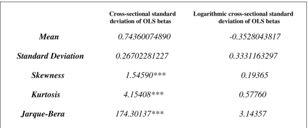
Herding model: Table 2 presents some statistics related to the estimated
cross-sectional standard deviation as well as the logarithmic cross-sectional standard deviation of the betas of the PSI-20 portfolio. As indicated by the table, the cross-sectional standard deviation of the betas is significantly different from zero and exhibits significant positive skewness and kurtosis, while the Jarque-Bera statistic indicates departures from normality (non-Gaussianity). When looking at the statistics of the logarithmic cross-sectional standard deviation of the betas, the above phenomena disappear. Therefore, the state-space model of Hwang and Salmon (2004) described previously can be legitimately estimated using the Kalman filter.
V. Results-Discussion
a) Positive feedback trading
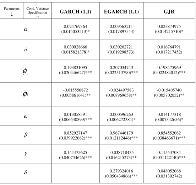
Table 3 presents the results from the Sentana and Wadhwani (1992) model-tests using the three variance-specifications mentioned above. The coefficients
describing the conditional variance process, ω,β, γ and δ , are all statistically significant (10% level) in all cases. Note also, that γ in the EGARCH-specification is negative and statistically significant (5%) implying that negative innovations tend to increase volatility more than positive ones. This is further confirmed by the -coefficient of the Asymmetric GARCH (1,1) which is positive (albeit insignificant). The feedback coefficient is indicative of statistically significant (5%) positive feedback trading for all three variance-specifications.
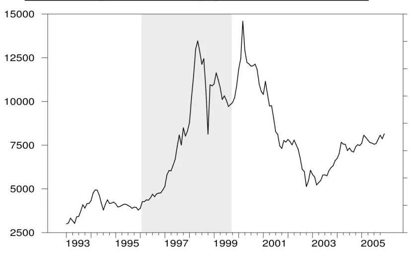
To see whether positive feedback trading exhibits statistical significance throughout the entire period of our sample, we run the model of Sentana and Wadhwani (1992) assuming 2-year rolling windows rolled every 30 days. Results indicated the presence of positive feedback trading, whose statistical significance is “clustered” around a certain period. More specifically, we found that positive feedback trading is found to be statistically significant (1%) during the 1996-1999 period which, as described previously (Section IV) corresponds to the “boom-bust” period for the Portuguese stock market11. These results are robust irrespective of the
GARCH-specification employed to test for the Sentana and Wadhwani (1992) model12; Figure 1 provides a graphic representation of these results.
b) Herding
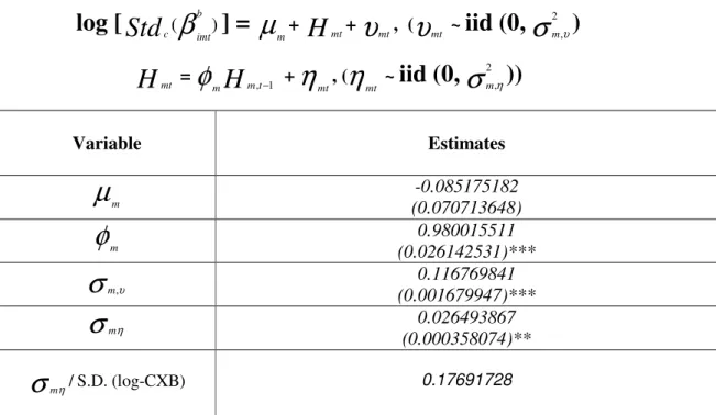
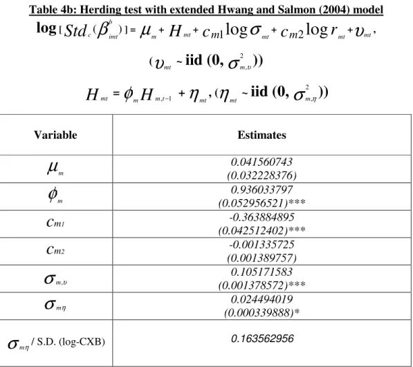
Tables 4a and 4b present the results related to herding on the premises of the Hwang and Salmon model, both the original one (Table 4a) as well as the extended one (Table 4b). According to those tables, both
φ
mand
σ
mη (the standard deviationof
η
mt) are statistically significant (10% level) and, thus it appears that there exists
herding towards the PSI-20 index. The bottom rows of Tables 4a-b provide us with the signal-proportion value, which according to Hwang and Salmon indicates what proportion of the variability of the logarithmic cross-sectional standard deviation of
11 We also run the Sentana and Wadhwani model using 3- and 4-year windows; the results obtained
were qualitatively similar to those generated by the 2-year windows.
12 Although each GARCH-specification is providing us with slight differences in the area of statistical
significance of positive feedback trading in the context of the Sentana and Wadhwani (1992) model, the area between January 1996 and September 1999 remains common among all three (GARCH(1,1), EGARCH, AGARCH(1,1) specifications across different rolling-window sizes.
the betas is explained by herding13. The signal-proportion value tends to hover around the same levels (approximately 17%) irrespective of the version of the Hwang and Salmon model used, which provides us with some evidence of robustness as to the presence of herding in the Portuguese market.
Although the signal-proportion value is well below the ones reported by Hwang and Salmon for the US and South Korean markets respectively14, it is hard to argue that there is less significant herding in Portugal compared to the US and South Korea, as Hwang and Salmon tested for herding on the premises of market indices, whose number of constituent stocks outnumber the one of the PSI-20 by far15.
It is interesting to note that Table 4b also reveals negative values for c1 and c2, thus indicating that the logarithmic cross-sectional deviation of the estimated betas tends to decrease as both market volatility and returns rise, although this relationship appears significant only with respect to market volatility. Since, according to Hwang and Salmon, herding appears as a reduction in the logarithmic cross-sectional dispersion of the estimated betas due to the
H
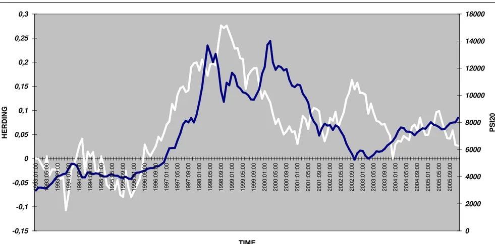
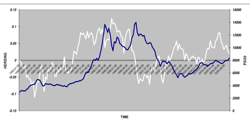
mt process, we interpret the above results as evidence of significant herd behaviour towards the PSI20, more so as the index exhibits higher volatility.Figures 2 and 3 present the evolution of herding diagrammatically (according to equation (12),
h
mt =1 – exp
(H
mt). We notice that herding assumes values wellbelow unity16, which indicates that extreme degrees of herding were not observed
during the 1993-2005 period.
The course of herding (represented by a white line in both Figures 2 and 3) compared to the PSI-20 index (represented by a dark line in both Figures 2 and 3) provides us with interesting insights. According to both charts, herding appears to be rising after January 1994, a rise which becomes more evident after December 1995 and continues up until October 1998. Following October 1998 herding exhibits a
13 The signal-proportion is estimated by dividing the
σ
ηm by the time series standard deviation of the
logarithmic cross-sectional standard deviation of the betas, in line with Hwang and Salmon (2004).
14 With the original herding model, Hwang and Salmon found that the value of the signal-proportion
was equal to approximately 44% for the US and South Korean markets; including the logarithmic market volatility and the index returns in the measurement equation, they came up with signal-proportion values equal to, approximately 32% for the US and 38% for the South Korean markets.
15 S&P500 for the US market and KOSPI for the Korean market. The KOSPI is an all-shares’ index;
Hwang and Salmon tested for herding in the Korean market based on 657 ordinary stocks listed on the KOSPI.
decline, whose direction asserts itself after October 1999. After January 2001, herding experiences certain fluctuations both upwards and downwards, without, however, managing to reach the pre-1999 levels. Overall, the picture seems to suggest that herding experienced a sharp rise during the pre-1999 boom-bust and started hovering around lower levels shortly after the “maturity” of the market.
We shall now try to delineate the course of herding compared to the PSI-20 over time on the basis of both Figures 2 and 3.
Herding exhibits a fall during 1993 (January-December), a year that coincides with the relaxation of restrictions on overseas capital flows and a sharp rise in foreign investment in Portuguese securities (Balbina and Martins (2002)). Herding starts rising (albeit with rather abrupt up- and down-fluctuations) throughout year 1994, reaching its highest level during the summer 1994, which corresponds to the outbreak of the Mexican crisis with its knock-on effects on international markets (Portugal included). This series of events, coupled with the poor corporate performance witnessed during that year (Balbina and Martins (2002)), could well have convinced the Portuguese investors of the negative prospects for the market, thus leading them to herd more. This is in line with Hwang and Salmon (2004), who found that herding is more pronounced during periods of “definitive” market direction, i.e. periods, when the course of the market clearly points towards a specific direction.
Following some fluctuations during 1995, herding sets onto an ascending course in December 1995. As Figures 2 and 3 illustrate, herding rallied with the PSI-20 for 2 ½ years (January 1996-April 1998) and continued its rally until October 1998. The herding peak coincides with the first bottom hit by the PSI-20 following the slump in May 1998. This implies that herding during this (roughly) three-year period kept growing as the market index skyrocketed (upward market direction) as well as when it bottomed (downward market direction). This constitutes evidence in favor of the aforementioned association between herding and “definitive” market direction postulated by Hwang and Salmon (2004). When the market was booming, investors were convinced of the rising trend and led herding levels to an unique (for the period under investigation) growth. In the advent of the Asian/Russian crises and their concomitant global impact, herding levels rose even more as these events may have led investors to believe that a market-reversal was imminent, thus leading the PSI-20 to its first bottom in October 1998.
Following year-end 1998, especially after September 1999, herding dwindled into lower levels with its descending course continuing until the beginning of year 2001. As mentioned previously, this period is characterized by a rather pronounced uncertainty (exacerbated by the international knock-on effects of the Asian/Russian crises) accompanied by a sudden rise of the index after September 1999 (US dotcom bubble-effect). It appears that herding towards the PSI-20 exhibited a free-fall during this period, as the index failed to produce a clear picture of a definitive directional movement.
After a series of fluctuations during most of 2001, herding shows some signs of ascension which culminates in increasing herding levels, especially between November 2001 and September 2002, only to drop abruptly again afterwards. This short rise in herding is associated with the bottom hit by the index following the peak of March 2000 and is found to commence shortly after the terrorist attack in New York on September, 11th 2001. Interestingly enough, Hwang and Salmon (2004)
report an increase in herding levels in the US-market following this event, which they associate with the advent of a “bearish” sentiment among US-investors. According to the above authors, this event may have functioned as a confirmation of a “bearish” market that was already underway following the NASDAQ’s slump in year 2000. The above may have impacted upon Portuguese investors as well, perhaps confirming the market drop that was underway in Portugal since March 2000. After the third quarter of 2002, herding starts falling again and begins to exhibit some signs of ascension during 2004 and 2005. However, as Figures 2 and 3 illustrate, herding during these two years has been mostly characterized by a rather volatile behaviour, without demonstrating any definitive directional movement.
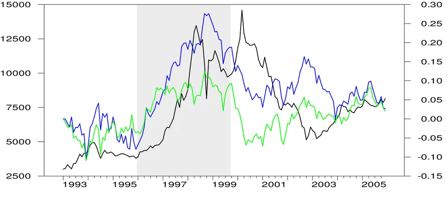
Our herding measure has, thus indicated that the boom-bust period (1996-1999) was characterized by a notably large rise in herding-levels, which never materialized again afterwards (until the end of our sample period). As this coincides with what has been noted previously for positive feedback trading (which was also found to be statistically significant during that same period), we also add Figure 4, which includes a combination of the results of our work for depiction purposes.
VI. Conclusion
Investors’ heterogeneity gives rise to complexity in the marketplace, as it leads to the interaction of a variety of strategies over time. Although heterogeneity is expected to maintain a sense of divergence within the market-participants’ ranks, this research suggests that convergence is also a valid possibility. Two forms of this potential “convergence” that have received extensive attention in Finance are herding and positive feedback trading. We have examined the presence of herding and positive feedback trading in the Portuguese stock exchange on the basis of the PSI-20 index during the 1993-2005 period. Our results indicate the presence of statistically significant herding and positive feedback trading during that period, which becomes more evident during the “boom-bust” period between 1996 and 1999. In line with Hwang and Salmon (2004), we find that herding tends to rise when the market exhibits a definitive direction and tends to decline when the market experiences fluctuations.
Appendix
Table 1: Sample statistics: PSI-20 daily returns (1/1/1993-31/12/2005) 0.03252137109 1.01772600552 S -0.63459*** K 7.68707*** LB(10) 117.9430919*** LB²(10) 766.0910101***
(* = 10% sign. Level, ** = 5% sign. Level, *** = 1% sign. Level). = mean, = standard deviation, S = skewness, K = excess kurtosis, LB (10) and LB² (10) are the Ljung-Box statistics for returns and squared returns respectively distributed as chi-square with 10 degrees of freedom.
Table 2: Sample statistics: Herding Measure (1/1/1993 to 31/12/2005)
Cross-sectional standard Logarithmic cross-sectional standard deviation of OLS betas deviation of OLS betas
Mean 0.74360074890 -0.3528043817 Standard Deviation 0.26702281227 0.3331163297 Skewness 1.54590*** 0.19365 Kurtosis 4.15408*** 0.57760 Jarque-Bera 174.30137*** 3.14357 (* = 10% sign. Level, ** = 5% sign. Level, *** = 1% sign. Level).
Table 3: Positive feedback trading tests (Sentana and Wadhwani (1992))
Parameters Cond. Variance
Specification GARCH (1,1) EGARCH (1,1) GJR
α (0.014053513)*0.024769364 (0.017897544)0.009563211 (0.014215710)*0.023874975 ϑ (0.015821378)*0.030028666 (0.019298573)0.030202721 (0.017217452)0.016764791
φ
0 0.193831095 (0.020446627)*** (0.022513790)***0.207034743 (0.022484012)***0.198475969φ
1 (0.005861641)**-0.015556872 (0.008969658)**-0.024497583 (0.005702052)**-0.015405740 ω 0.013058591 (0.006530899)*** (0.006272384)*0.000596263 (0.007342656)* 0.014177318 β 0.852927147 (0.039922082)*** (0.012112446)***0.967446179 (0.038463671)***0.854552062 γ 0.144475625 (0.040734626)*** (0.016215273)**-0.038718435 (0.031122140)***0.115537084 δ 0.279324016 (0.050434866)*** (0.031302742)0.048052068(* = 10% sign. Level, ** = 5% sign. Level, *** = 1% sign. Level). Parentheses include the standard errors of the estimates; sample period: 1/1/1993-31/12/2005.
Table 4a: Herding test with original Hwang and Salmon (2004) model
log [
(β
b ) imt cStd
] =
µ
m+H
mt+υ
mt, (υ
mt ~iid (0,
σ
υ 2 , m)
H
mt =φ
mH
m,t−1 +η
mt, (η
mt ~iid (0,
σ
η 2 , m))
Variable Estimatesµ
m (0.070713648) -0.085175182φ
m (0.026142531)*** 0.980015511σ
m,υ (0.001679947)*** 0.116769841σ
mη 0.026493867 (0.000358074)**σ
mη/S.D. (log-CXB) 0.17691728(* = 10% sign. Level, ** = 5% sign. Level, *** = 1% sign. Level). Parentheses include the standard errors of the estimates; sample period: 1/1/1993-31/12/2005.
Table 4b: Herding test with extended Hwang and Salmon (2004) model
log
[ (β
b ) imt cStd
] =µ
m+H
mt+c
m1log
σ
mt+c
m2log
r
mt+υ
mt, (υ
mt ~iid (0,
σ
2m,υ))
H
mt =φ
mH
m,t−1 +η
mt, (η
mt ~iid (0,
σ
η 2 , m))
Variable Estimatesµ
m (0.032228376) 0.041560743φ
m (0.052956521)*** 0.936033797c
m1 -0.363884895 (0.042512402)***c
m2 -0.001335725 (0.001389757)σ
m,υ (0.001378572)*** 0.105171583σ
mη 0.024494019 (0.000339888)*σ
mη/ S.D. (log-CXB) 0.163562956(* = 10% sign. Level, ** = 5% sign. Level, *** = 1% sign. Level). Parentheses include the standard errors of the estimates; sample period: 1/1/1993-31/12/2005.
25
Figure 1: Area of positive feedback trading significance for the PSI-20 (1993-2005)
1993
1995
1997
1999
2001
2003
2005
2500
5000
7500
10000
12500
15000
-1.00
-0.75
-0.50
-0.25
0.00
0.25
0.50
0.75
1.00
Figure 2: Herding towards the PSI-20 (testing with original Hwang and Salmon (2004) model)
-0,15 -0,1 -0,05 0 0,05 0,1 0,15 0,2 0,25 0,3 19 93 :0 1: 00 19 93 :0 5: 00 19 93 :0 9: 00 19 94 :0 1: 00 19 94 :0 5: 00 19 94 :0 9: 00 19 95 :0 1: 00 19 95 :0 5: 00 19 95 :0 9: 00 19 96 :0 1: 00 19 96 :0 5: 00 19 96 :0 9: 00 19 97 :0 1: 00 19 97 :0 5: 00 19 97 :0 9: 00 19 98 :0 1: 00 19 98 :0 5: 00 19 98 :0 9: 00 19 99 :0 1: 00 19 99 :0 5: 00 19 99 :0 9: 00 20 00 :0 1: 00 20 00 :0 5: 00 20 00 :0 9: 00 20 01 :0 1: 00 20 01 :0 5: 00 20 01 :0 9: 00 20 02 :0 1: 00 20 02 :0 5: 00 20 02 :0 9: 00 20 03 :0 1: 00 20 03 :0 5: 00 20 03 :0 9: 00 20 04 :0 1: 00 20 04 :0 5: 00 20 04 :0 9: 00 20 05 :0 1: 00 20 05 :0 5: 00 20 05 :0 9: 00 TIME H E R D IN G 0 2000 4000 6000 8000 10000 12000 14000 16000 P S I2 0Herding = white line PSI-20 = dark line
27
Figure 3: Herding towards the PSI-20 (testing with extended Hwang and Salmon (2004) model)
-0.15 -0.1 -0.05 0 0.05 0.1 0.15 1993 :01:00 1993 :05:00 1993 :09:00 1994 :01:00 1994 :05:00 1994 :09:00 1995 :01:00 1995 :05:00 1995 :09:00 1996 :01:00 1996 :05:00 1996 :09:00 1997 :01:00 1997 :05:00 1997 :09:00 1998 :01:00 1998 :05:00 1998 :09:00 1999 :01:00 1999 :05:00 1999 :09:00 2000 :01:00 2000 :05:00 2000 :09:00 2001 :01:00 2001 :05:00 2001 :09:00 2002 :01:00 2002 :05:00 2002 :09:00 2003 :01:00 2003 :05:00 2003 :09:00 2004 :01:00 2004 :05:00 2004 :09:00 2005 :01:00 2005 :05:00 2005 :09:00 TIME H E R D IN G 0 2000 4000 6000 8000 10000 12000 14000 16000 P S I2 0
Herding = white line PSI-20 = dark line
Figure 4: Herding and positive feedback trading towards the PSI20
1993 1995 1997 1999 2001 2003 2005 2500 5000 7500 10000 12500 15000 -0.15 -0.10 -0.05 0.00 0.05 0.10 0.15 0.20 0.25 0.30Herding (original model of Hwang and Salmon) = blue line, Herding (extended model of Hwang and Salmon) = green line PSI-20 = black line
References
1) Andergassen, R.,2003, “Rational destabilizing speculation and the riding of bubbles, Working Paper, Department of Economics, Univ. of Bologna.
2) Antoniou, A., Koutmos, G. and Pericli, A., 2005,“Index Futures and Positive Feedback Trading: Evidence from Major Stock Exchanges”, Journal of Empirical Finance, Vol.12, Issue 2, pp. 219-238.
3) Arthur, W.B., 1994, "Inductive Reasoning and Bounded Rationality," American Economic Review, A.E.A. Papers and Proc.), 84, pp. 406-411
4) Arthur, W.B.: "The Economy as an Evolving Complex System II.," W. Brian Arthur, Steven N. Durlauf, and David A. Lane, (Eds.), Proceedings Volume XXVII, Santa Fe Institute Studies in the Science of Complexity, Reading, MA: Addison-Wesley, 1997. Review by Gerald Silverberg, Maastricht.
5) Arthur, W.B., 2000a,”Complexity and the Economy”, Science, April 1999, 284, 107-109. Reprinted in The Complexity Vision and the Teaching of Economics, D. Colander, ed., Edward Elgar Publisher.
6) Arthur, W.B., 2000b,” Cognition: The Black Box of Economics," The Complexity Vision and the Teaching of Economics, David Colander, ed., Edward Elgar Publishing, Northampton, Mass.
7) Arthur, W.B.,: "The End of Certainty in Economics," Talk delivered at the conference Einstein Meets Magritte, Free University of Brussels, 1994. Appeared in “Einstein Meets Magritte”, D. Aerts, J. Broekaert, E. Mathijs, eds. 1999, Kluwer Academic Publishers, Holland. Reprinted in The Biology of Business, J.H. Clippinger, 1999, Jossey-Bass Publishers.
8) Balbina and Martins, 2002,“The Analysis of Seasonal Anomalies in the Portuguese Stock Market”, The Bank of Portugal
9) Banerjee, A. V., 1992, “A simple model of herd behavior”, The Quarterly Journal of Economics, Vol. CVII, Issue 3, pp. 797-817.
10) Barberis, N., Shleifer, A. and Vishny, R., 1998, “ A model of investor sentiment“, Journal of Financial Economics, 49, pp. 307-343.
11) Barberis, N. and Thaler, R., 2002, ” A survey of behavioural finance”, National Bureau of Economic Research Working Paper 9222.
12) Bikhchandani, S., Hirshleifer, D. and Welch, I., 1992, “A theory of fads, fashion, custom, and cultural change as informational cascades”, Journal of Political Economy, Vol. 100, No. 5, pp. 992-1026
13) Bikhchandani S. and Sharma S., 2001, ”Herd Behaviour in Financial Markets”, IMF Staff Papers, Vol. 47, No3
14) Bohl, M. T. & Reitz, S, 2002, “The influence of positive feedback trading on return autocorrelation: evidence from the German stock market”, Working Paper, European University Viadrina Frankfurt (Oder)
15) Bohl, M. T. & Reitz, S. ,2003, “Do positive feedback traders act in Germany’s Neuer Markt?”, Working Paper, European University Viadrina Frankfurt (Oder) 16) Bollerslev, T., R.F Engle and D. Nelson, 1994, ARCH Models, in R.F. Engle and D.L.McFadden, eds, Handbook of Econometrics, Vol IV (Elsevier Science B.V.) Ch 49. 17) Brooks, C.: “Introductory Econometrics for Finance”, Cambridge, 2002.
18) Chang, E.C., Cheng, J.W. and Khorana, A., 2000,” An examination of herd behaviour in equity markets: An international perspective”, Journal of Banking and Finance, 24, pp. 1651-1679
19) Christie, W.G. and Huang, R.D., 1995, “Following the Pied Piper: Do Individual Returns Herd around the Market?”, Financial Analysts Journal, pp.31-37.
20) De Bondt, W. F. M. and Teh, L. L., 1997, « Herding behavior and stock returns : an exploratory investigation », Swiss Journal of Economics and Statistics, Vol. 133 (2/2), pp. 293-324
21) De Long, J.B., Shleifer, A., Summers, L.H. and Waldmann, R.J., 1990, “Positive Feedback Investment Strategies and Destabilizing Rational Speculation”, The Journal of Finance, Volume 45, Issue 2, pp. 379-395.
22) Devenow, A. and Welch, I., 2004, “ Rational herding in financial economics” European Economic Review, 40, pp. 603-615.
23) Fama, E. and French, K.R., 1993, “Common risk factors in the returns on stocks and bonds”. Journal of Financial Economics 33, pp. 3–56
24) Farmer, J.D., 2001, “Toward Agent-Based Models for Investment”, Association for Investment Management and Research.
25) Farmer, J.D., 2002, “Market force, ecology and evolution”, Industrial and Corporate Change, Vol. 11, No.5, pp. 895-953 (59).
26) Farmer, J.D. and Lo, A.W., 1999, “ Frontiers of Finance: Evolution and Efficient Markets”.
27) Glaser, M. and Weber, M., 2004a, “Overconfidence and Trading Volume“, Sonderforschungsbereich 504 Working Paper No. 03-07.
28) Glaser, M. and Weber, M., 2004b, “Which Past Returns Affect Trading Volume? “, Sonderforschungsbereich 504 Working Paper.
29) Glosten L, Jagannathan R, and Runkle D, 1993, “Relationship between the Expected Value and the Volatility of the Nominal Excess Return on Stocks”, Journal of Finance, 48, 1779-1801.
30) Graham, J.R., 1999, ”Herding among Investment Newsletters: Theory and Evidence”, The Journal of Finance, Vol. LIV, No. 1, pp.237-268
31) Hirshleifer, D., 2001, “Investor Psychology and Asset Pricing”, Journal of Finance, Vol. LVI, No4.
32) Hirshleifer, D. and Teoh, S.T., 2003, ”Herd Behaviour and Cascading in Capital Markets: a Review and Synthesis”, European Financial Management Journal, Vol. 9, No. 1, pp. 25-66.
33) Huddart, S., Lang, M. and Yetman,M., 2002, ” Psychological factors, stock price paths and trading volume.” Pennsylvania State University.
34) Hwang, S. and Salmon, M., 2004, “Market stress and herding”, Journal of Empirical Finance, 11, pp. 585-616.
35) Koutmos, G., 1997, ”Feedback trading and the autocorrelation pattern of stock returns: further empirical evidence”, Journal of International Money and Finance, Vol. 16, No. 4, pp. 625-636.
36) Koutmos, G. and Saidi, R., 2002, “Positive feedback trading in emerging capital markets”, Applied Financial Economics, 11, 291-297.
37) Kyle, A.S. and Wang, F.A., 1997, ” Speculation Duopoly with Agreement to Disagree: Can Overconfidence Survive the Market Test? ”, The Journal of Finance, Vol. LII, No. 5, pp.2073-2090.
38) Lakonishok, J., Shleifer, A. and Vishny, R., 1992, ”The impact of institutional trading on stock prices”, Journal of Financial Economics, 32, pp. 23-43.
39) Lobao, J. & Serra, A.P., 2002,” Herding Behaviour: Evidence from Portuguese Mutual Funds”, CEMPRE, Faculdade de Economia do Porto
40) Mauboussin, M.J., 2002, “ Revisiting market efficiency: the stock market as a complex adaptive system”, Journal of Applied Corporate Finance, Vol. 14, No. 4, pp.8-16.
41) Nelson, D.B., 1991, “Conditional Heteroscedasticity in asset returns: A new approach”, Econometrica, 59(2), pp. 347-370.
42) Odean, T., 1998, ” Volume, Volatility, Price and Profit when all traders are above average”, The Journal of Finance, Vol LIII, No. 6.
43) Osler, C.L., 2002, “Stop-loss Orders and price cascades in currency markets”, The Federal Reserve Bank of New York, Staff Report No. 150.
44) Scharfstein and Stein, 1990, “Herd Behaviour and Investment“, The American Economic Review, Volume 80, Issue 3, pp. 465-479
45) Schwert G.W., 1989, “Why does stock market volatility change over time?”, Journal of Finance 44, pp. 1115–1153.
46) Sentana, E. and Wadhwani, S., 1992, ” Feedback Traders and Stock Return Autocorrelations: Evidence from a Century of Daily Data”, “The Economic Journal”, Volume 102, Issue 411, pp. 415-425.
47) Shiller, R. J., 1995, “Conversation, Information and Herd Behavior” American Economic Review, 85(2), pp. 181–185.”
48) Sousa, A, 2002, “A Evolução do Mercado de Acções em Portugal”, Mestrado em Economia, Faculdade de Economia, Universidade de Coimbra.
49) Trueman, Brett, 1994, “Analyst Forecasts and Herding Behaviour”, The Review of Financial Studies,Vol.7, No.1, pp.97-124
50) Wermers, Russ, 1999, ”Mutual Fund Herding and the Impact on Stock Prices”, The Journal of Finance, Vol. LIV, No.2, pp. 581-622.