Disorder and localization effects in correlated electronic systems

Vítor Manuel Pereira

Disorder and Localization Effects in

Correlated Electronic Systems

Departamento de Física

Faculdade de Ciências da Universidade do Porto

October 2006

Vítor Manuel Pereira

Disorder and Localization Effects in

Correlated Electronic Systems

Departamento de Física

Faculdade de Ciências da Universidade do Porto

October 2006

Vítor Manuel Pereira

Disorder and Localization Effects in

Correlated Electronic Systems

Tese submetida à Faculdade de Ciências da Universidade do Porto para obtenção do grau de Doutor em Física

faculdade de Ciências do rorfo

oibiioltcs do Departamento de ítsica

Departamento de Física

Faculdade de Ciências da Universidade do Porto

October 2006

Acknowledgements

I am most indebted to many people who, knowingly or not, have helped me throughout these doctoral years. It all starts with the privilege of working with my supervisor for the doctoral program at FCUP, professor João M. B. Lopes dos Santos, my mentor since the graduation years, and with whom there is always so much to learn, investigate and discuss (be the subject condensed matter theory or pretty much anything else). It is, and I am shure will always be, a pleasure to do physics with you.

When my PhD program had barely started, I came to meet professor Antonio H. Castro Neto, my su-pervisor at Boston University (BU). Staying in Boston under his attention was perhaps my most important experience as a training physicist. For many reasons, that include the quality of the scientific research and scientific debate at BU, my supervisor's expertise as a leading condensed matter theorist, but mostly from my personal contact with prof. Castro Neto's disturbingly unbreakable good spirits and optimism, which only seem to grow with the difficulties at hand, and readily spread among its collaborators.

At several stages, I benefited from discussing my ongoing work with other people. Among them, and for their precious insights, comments or suggestions, I would like to mention Leo Degiorgi (ETH), Paco Guinea (ICMM, Madrid), Nuno Peres (Universidade do Minho), Yuri G. Pogorelov (FCUP), Eduardo Castro (FCUP), Eduardo Novais (Duke University), Marcello Silva Neto (University of Utrecht), Peter Littlewood (Cambridge University) and Anders Sandvik (Boston University).

I acknowledge Boston University and its Department of Physics, for all the institutional and practical support during my four half-year stays at BU, including the access to the scientific computing facilities. Likewise, I recognize the support of the Department of Physics at FCUP, especially for their invitation to a teaching assistant position during the last year, and Centro de Física do Porto, for all financial, office and computational support.

I thank my family, Tânia's and my friends; I thank B. J. Teitleman for always insisting upon showing me the other side of things; my fellow students and post-doctoral researchers both at BU (especially the Brazilian contingent who helped me settle during the first weeks); and my fellow graduate students in Porto (mathematicians included, of course). Thanks to Miguel for the tips and suggestions about everything, especially on how to use OpenMP to get your code scheduled at 200% CPU. I would also like to mention Anton Kozlov, and David Sheridan, who is an amazing source of american culture, and did his best at coaching me how to strike a good hard liner.

My PhD activities, including the travelling expenses between Porto and Boston, would not have been possible without the doctoral grant from Fundação para a Ciência e a Tecnologia, under the reference SFRH/BD/465 5/2001, and to which I am most grateful indeed.

Last, but foremost, as always, I mention you, Tânia. In particular because...

Abstract

This thesis is about electrons in disordered structures, and electrons correlated with other degrees of freedom. In particular, the discussions and results in the ensuing chapters pertain to two main categories that can be summarily synthesized as electrons interacting with localized magnetic moments - as in the DEM - and electrons in disordered two dimensional carbon.

Double Exchange Model (DEM). With regard to the DEM, we discuss in detail the region of validity of the

DE limit for magnetic systems described by a Kondo lattice Hamiltonian, putting in perspective the two opposed limits J —v oo and J —► 0, and concluding that the former appears as the best approximation in the intermediate coupling regime. For DE systems with low densities of electronic carriers, the effects of Anderson localization are found here to be of paramount relevance. In that context we provide the first mapping of the mobility edge, Ec, as a function of the local spin magnetization in this system, and show that such magnetization dependent Ec has profound consequences to the magneto­transport response, including CMR effects, strongly enhanced electrical conductivities in the ferromagnetic phase, or blue­shifts of the plasma edge in the optical reflectivity.

The stability of free magnetic polarons in the pure low density DEM is addressed both phenomenologically and numerically. It is found that, at low densities, the PM­FM transition is mediated by a polaronic phase, which has the effect of considerably reducing the Curie temperatures, Tc, with respect to the mean­field estimates. At the same time, we analyze the related problem of phase separation in this same low density regime. We demonstrate that the phase separation instability characteristic of this model is strongly suppressed when electrostatic and localization corrections are included in the free energy, and establish a connection between the resulting ground state and the non­interacting polaronic phase.

Magnetic Hexaborides. A microscopic theory forrare­earth ferromagnetic hexaborides, of the type Eui_xCaxB6,

is proposed on the basis of the DE Hamiltonian. In these compounds, the reduced carrier concentrations place the Fermi level near the mobility edge, introduced in the spectral density by the disordered spin background. We show that some of their puzzling experimental signatures, such as the Hall effect, magnetoresistance, frequency dependent conductivity, and dc resistivity can be quantitatively described and coherently understood within the model. The region of magnetic polaron stability detected through Raman scattering experiments is also well re­ produced, and we make specific predictions as to the behavior of the Curie temperature as a function of the plasma frequency, proposing a phase diagram for the doped family. We also discuss how recent transport and magneto­ optical measurements confirm our Double Exchange (DE)­based picture and reproduce our originally proposed phase diagram.

Anderson Localization. We present evidence regarding the relevance of the local environment statistics in the

phenomenon of Anderson localization. It is shown that the fluctuations in the inverse participation ratio, or in the local density of states, exhibit critical behavior, and provide strong evidence supporting the LDOS as an order parameter for the Anderson transition.

Graphene. Our incursion onto the subject of two dimensional carbon, reveals the consequences of different

types of disorder for the electronic structure of graphene. We underline, in particular, the case of vacancies, which are shown to induce the emergence of localized modes at the Fermi energy, with a huge concomitant enhancement of the density of states. The relevance of these results in the explanation of the magnetism detected in disordered graphite is addressed.

Resumo

A presente tese é dedicada ao estudo de electrões em estruturas desordenadas, e electrões correlacionados com outros graus de liberdade. Em particular, as discussões e resultados apresentados nos capítulos seguintes poderão organizar-se segundo duas categorias principais, nomeadamente electrões interagindo com momentos magnéticos locais - tal como no MDT - e electrões no carbono bidimensional com desordem.

Modelo de Dupla Troca (MDT). Relativamente ao MDT, o regime de validade do limite de dupla troca é

dis-cutido em detalhe no âmbito de sistemas descritos pela rede de Kondo, colocando-se em perspectiva os limites J — K » e . / - í O , e concluindo-se acerca da melhor aplicabilidade do primeiro nos casos de acoplamento intermé-dio. Para sistemas de DT com uma densidade baixa de portadores, mostra-se que os efeitos associados à localização de Anderson são de máxima relevância. Nesse contexto, é apresentada a primeira trajectória do limiar de mobi-lidade, Ec, como função da magnetização local para este problema, mostrando-se ainda que a existência de um limiar de mobilidade dependente da magnetização tem profundas consequências na resposta eléctrica e magnética do sistema, incluindo o aparecimento de efeitos de magnetorresistência colossal, condutividades dramaticamente amplificadas na fase ferromagnética, ou desvios para o azul na frequência de plasma.

A estabilidade de polarões magnéticos no MDT a baixa densidade é estudada fenomenológica e numericamente. Decorre dos resultados que, a baixas densidades, a transição PM-FM é mediada por uma fase polarónica, donde decorre um abaixamento considerável das temperaturas de Curie, Tc, relativamente às estimativas típicas de campo médio. Ao mesmo tempo, é abordada a questão da separação de fases no MDT. Demonstra-se que a instabilidade subjacente à separação de fases é fortemente suprimida através da inclusão de contribuições electrostáticas e de localização na energia livre, evidenciando-se ainda as similaridades entre o estado fundamental daí resultante e a fase polarónica.

Hexaboretos magnéticos. No âmbito dos hexaboretos de európio do tipo Eui_xCaxB6, é proposto um

mo-delo microscópico alicerçado no MDT. Nestes compostos, a reduzida densidade electrónica implica a significativa proximidade entre o nível de Fermi e o limiar de mobilidade induzido pela desordem magnética. Mostra-se aqui que as intrigantes características experimentais destes hexaboretos, como sejam o efeito Hall, a magnetorresistên-cia, a condutividade óptica ou a resistividade, podem ser descritas e entendidas de modo coerente com base nesse modelo. A região de estabilidade polarónica registada em medidas Raman é igualmente bem reproduzida pelo cor-respondente diagrama de fases do MDT, sendo ainda proposto o diagrama de fases para os hexaboretos dopados. Finalmente, discute-se como este modelo e o diagrama de fases proposto vêm a ser corroborados por resultados experimentais subsequentes.

Localização. Entre os nossos resultados, são avançadas provas relativas à importância das propriedades locais

no processo de localização de Anderson. Mostra-se que tanto a fracção de orbitais que contribuem para um dado autoestado, como a densidade local de estados, exibem flutuações com comportamento crítico, dando força a uma interpretação da densidade local de estados como possível parâmetro de ordem na transição de Anderson.

Grafeno. A incursão no tópico do carbono bidimensional revela algumas das consequências que diferentes

modelos de desordem trazem para a estrutura electrónica do grafeno. É destacado, em particular, o caso de lacunas, das quais resultam estados localizados no nível de Fermi, ao mesmo tempo que fazem surgir um pico significativo na densidade de estados em EF. O significado destes resultados para a compreensão do magnetismo detectado em

amostras de grafite é discutido no final.

Résumé

Le sujet de cette thèse est les électrons en structures désordonnées, et les électrons corrélées avec d'autres degrés de liberté. En particulier, les discussions et les résultats dans les chapitres suivants concernent deux catégories principales qui peuvent être sommairement synthétisées comme des électrons en interaction avec des moments magnétiques localisés - comme dans le MDE - et des électrons dans le carbone bidimensionnel désordonné.

Modèle du Double Échange (MDE). En qui concerne le MDE, on discute en détail la région de validité du

limite de DE pour des systèmes magnétiques décrits par un Hamiltonien de Kondo, et on compare les deux limites opposées, J —> oo et J —» 0, en concluant que le premier apparaît comme une meilleure approximation dans le régime d'accouplement intermédiaire. Pour des systèmes avec de faibles densités des électrons, les effets de localisation d'Anderson ont une importance primordiale. Dans ce contexte on fournisse la dépendance du bord de mobilité, Ec, en fonction de la magnétisation du système, et nous prouvons qu'une telle dépendance a des conséquences profondes sur la réponse magnétique et électrique, comme par exemple, des effets de CMR, des conductivités fortement augmentées dans la phase ferromagnétique, ou le décalage vers le bleu de la fréquence de plasma dans la réflectivité optique.

La stabilité des polarons magnétiques dans le MDE est adressée phénoménologique et numériquement. On constate que, pour des faibles densités, la transition PM-FM est interpolée par une phase polaronique qui a l'effet d'une considérable réduction des températures de Curie, Te, vis-a-vis les valeurs obtenus en champ moyen. En même temps, on étude le problème de la séparation et coexistence des phases dans ce même régime de faible densité. On démontre que l'instabilité vers la séparation des phases caractéristique de ce modèle est fortement supprimée sur l'effet des contributions électrostatiques et de localisation dans l'énergie libre, et on établisse une liaison entre l'état fondamental résultant et la phase polaronique.

Hexaborures magnétiques. On propose une théorie microscopique pour les Hexaborures ferromagnétiques, du

type Eui_xCaxB6, basée sur le Hamiltonien de DE. Dans ces substances, pour vue de la faible concentration

d'électrons, le niveau de Fermi et le bord de mobilité se trouvent très proches. On montre que la majorité de leur signatures expérimentales, comme l'effet de Hall, la magnetorésistance colossale, la conductivité optique, et la résistivité peuvent être quantitativement décrites et entendus dune façon cohérente avec ce modèle. La région de stabilité des polarons magnétiques détectée par Raman est également reproduite, et nous faisons des prévisions spécifiques en ce qui concerne le comportement relatif entre la température de Curie et la fréquence de plasma, proposant le diagramme de phase pour la famille dopée. On discute également les récentes expériences magnéto-optiques que confirment notre scénario théorique basé dans le MDE, et reproduisent le diagramme de phase.

Localisation d'Anderson. On présente des évidences concernant la pertinence de l'environnement local dans le

phénomène de la localisation d'Anderson. On montre que les fluctuations dans le rapport inverse de participation, ou dans la densité locale d'états ont un comportement critique, et fournissent évidence soutenant la densité locale d'états comme paramètre d'ordre pour la transition d'Anderson.

Graphène. Notre incursion dans le sujet du carbone bidimensionnel montre les conséquences que différents

modeles de désordre peuvent avoir dans la structure électronique de graphène. Nous accentuons, en particulier, le cas de lacunes, qui donnent lieu a l'émergence des modes localisés à l'énergie de Fermi, au même temps qu'une énorme résonance apparaît dans la densité d'états. La pertinence de ces résultats pour une explication du magnétisme détecté en graphite désordonné est adressée.

Contents

Acknowledgements v

Abstracts vii Contents xvi List of Figures xix List of Acronyms xxi 1. Introduction 3

1.1. Context 3 1.2. Organization of the Thesis 4

1.3. Original Content and External Material 5

2. The Recursive Method 7

2.1. Introduction 7 2.1.1. When k-space will not do 7

2.1.2. Local electronic structure 8

2.1.3. Why Recur? 9 2.2. The Chain Model and the Tridiagonalization Scheme 10

2.2.1. Transformation to a chain 10 2.2.2. Exact diagonalization and orthogonal polynomials 14

2.3. Local Density of States and Green Functions 18

2.3.1. Green Functions 18 2.3.2. Continued Fraction Representation 19

2.3.3. Processing the Continued fraction 21 2.3.3.1. The Square Root Terminator 22 2.3.3.2. Delta Function Broadening 24 2.3.3.3. Integrated Quantities and Re-differentiation 26

2.4. Gapped and Disordered Systems 30 2.4.1. Singularities and Asymptotic Behavior of the Continued Fraction 30

2.4.2. Band Gaps and the asymptotic problem 31

2.4.3. Stochastic Recursive Method 33

2.5. Numerical Caveats 36 xiii

xiv CONTENTS

2.5.1. Versatility from a smart choice of the starting state 36

2.5.2. On the chain model 37 2.5.3. On the calculation of the LDOS 38

Appendices for this chapter 41 2.A. On the Sturm property of the leading minors 41

2.B. The truncated CF and Padé approximants 42 2.C. The CF expansion and Dyson's equation 43

2.D. DOS from the average LDOS 44 3. EuB6: Background and Significance 47

3.1. Crystal Structure 47 3.2. Theoretical Electronic Structure 48

3.3. Experimental Electronic Structure 49

3.4. Magnetism 52 3.5. Transport 52 3.6. Optical Response 55

3.7. Doping EuB6 56 Appendices for this chapter 59

3.A. A word on the magnetism of CaB6 59 4. The DEM and Magnetic Hexaborides 61

4.1. The Basic Premises 61 4.1.1. Estimation of Parameters 62

4.2. The Double Exchange Model at Low Density 63

4.2.1. The DE Hamiltonian 63 4.2.2. The DE Regime 66 4.3. Magnetic Disorder in the DEM 71

4.3.1. Hybrid Thermodynamic Approach 72

4.3.2. Anderson Localization 75 4.3.2.1. Full Diagonalization — Wavefunction Based 76

4.3.2.2. Local Environment — LDOS Fluctuations 82

4.3.2.3. Trajectory of the Mobility Edge 86

4.3.3. Spectral and Transport Properties 87 4.3.3.1. Single Particle Spectral Function 87

4.3.3.2. Mobility Gap, Extended and Localized Carriers 91

4.3.3.3. Electrical Resistivity 95 4.3.3.4. Optical Response: The Plasma Edge 96

4.4. The DE interpretation of Eui-xCa^Be 102 4.4.1. Recent Experimental Developments 105

Contents xv

Appendices for this chapter 107 4.A. Bilinear Fermionic Commutators 107 4.B. DEM: Projecting out the high energy scales 108

4.C. KLM within a Virtual Crystal Approximation 110 4.D. Average hoppings within mean field 112

4.E. IPR Statistics - Additional Results 115 4.F. Lifetime within perturbation theory for the Anderson model 116

5. Magnetic Polarons and Phase Separation 119

5.1. Magnetic Polarons in the DEM 119 5.1.1. Magnetic Polarons in Perspective 119

5.1.2. The Independent Polaron Model 120 5.1.3. The Polaronic Evidence in EuB6 124 5.2. The Problem of Phase Separation 125

5.2.1. Canonical Free Energy and Phase Diagram 125

5.2.2. The Essence of the Problem 126 5.2.3. Electrostatic Suppression of Phase Separation 130

5.2.3.1. Electrostatic Correction 130 5.2.3.2. Phase Space Correction 132 5.2.4. Consequences to the Phase Diagram 133

5.2.4.1. Phase Separation and Magnetic Polarons 134 5.2.5. General Argument Regarding Phase Separation 135

Appendices for this chapter 139 5.A. Effects of Finite Band Filling on Polaron Stability 139

5.B. Finite Size Corrections to the Electronic DOS 140

6. Two Dimensional Carbon 143 6.1. A Two Dimensional Solid Made Reality 143

6.2. Electrons in a Honeycomb Lattice 145 6.3. Disorder and Localization in Graphene 149

6.3.1. Relevance of Disorder in Graphene 149

6.3.2. Vacancies 149 6.3.2.1. Vacancies and a theorem 150

6.3.2.2. Numerical Results 152

6.3.3. Selective Dilution 156 6.3.4. Local Impurities 160 6.3.5. Non-Diagonal Impurities 161

6.4. Implications for real systems 164

xvi CONTENTS

A. Relevant Publications by the Author 167

List of Figures

2.1. Selected chain states for the tight-binding model in 2D 13

2.2. Selected chains states of different symmetry 13

2.3. Chain transformation 22 2.4. Numerical example for the 3D tight-binding Hamiltonian 24

2.5. Numerical example for the 2D tight-binding Hamiltonian 25 2.6. Constructing the DOS from broadening of the chain levels 25

2.7. Crude approximation to the integrated DOS 27 2.8. Quadrature technique applied to the integrated DOS 28

2.9. Integrated DOS for the 3D tight-binding from quadrature 29

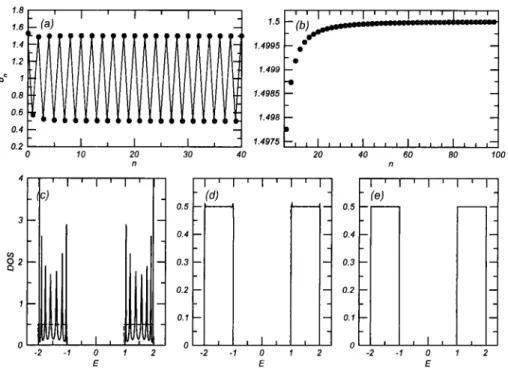
2.10. DOS from quadrature on a 3D cubic lattice 30 2.11. Matching of the terminator and effective medium (schematic) 30

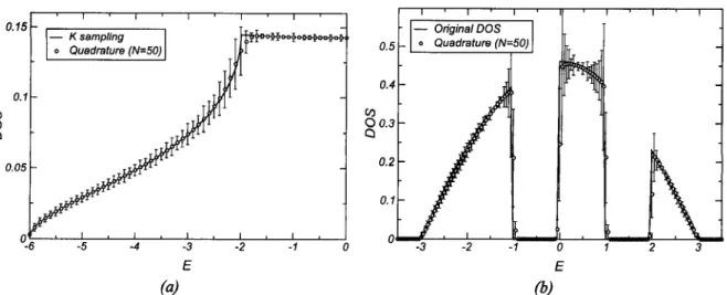
2.12. Recursive coefficients for a gapped square band 32 2.13. Recursive method applied to a gapped band 34 2.14. DOS of the 2D tight-binding model: recursion vs if-sampling 35

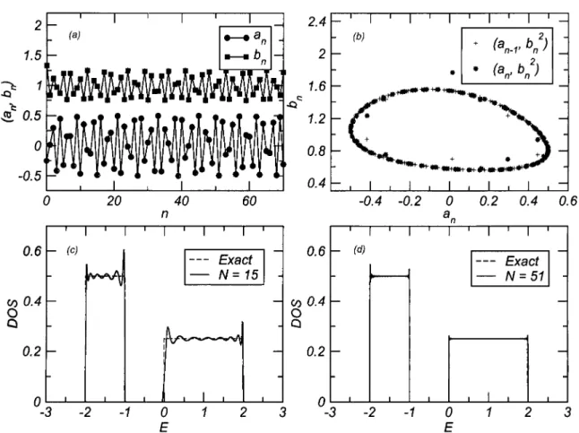
2.15. DOS for the Anderson model in 2D 36

2.16. Orthogonal Polynomials 41 2.17. Diagrammatic expansion and Dyson's equation 44

3.1. Crystal structure ofEuBg 48 3.2. Several DFT results for the bandstructure of hexaborides 50

3.3. Experimental band structure 51 3.4. Magnetic response of EuE$6 53 3.5. Transport and mageto-transport properties 54

3.6. Magneto-optical response ofEuBg 55

3.7. Raman scattering in EUBÔ 57

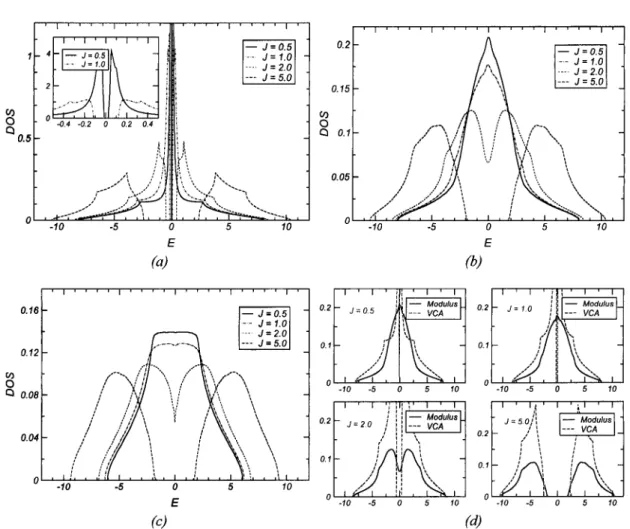
3.8. Consequences of doping upon the magneto-transport of Eui_xCaxB6 58 4.1. Schematic representation of global and local quantization axes 64 4.2. DOS for the KLM in the PM phase within several approximations 68

4.3. Examples of projected DOS 69 4.4. Local polarization per electron in the KLM 70

4.5. DOS for the DEM at different magnetizations 74 4.6. Schematic models of disorder and mobility edge 75 4.7. Spectrum and wavefunctions from full diagonalization of the DEM 77

x v i i i LIST OF FIGURES

4.8. IPR statistics in the DEM 80 4.9. Relative fluctuations in the IPR 81 4.10. LDOS distributions in the DEM and AM 83

4.11. LDOS fluctuations in the DEM and AM 84

4.12. Typical DOS 85 4.13. Localized wavefunctions (schematic) 85

4.14. Mobility edge trajectory for the DEM and AM 87 4.15. Single particle spectral function in the DEM along the cubic BZ 89

4.16. Inverse single-particle lifetimes in the AM and DEM 90

4.17. Density of localized states in the DEM 92 4.18. Mobility gap, Fermi energy and extended states in EuB6 94

4.19. Conduction states and resistivity: theory vs experiment 95

4.20. Plasma Frequency vs Magnetization 100 4.21. Proposed phase diagram for Eui-^Ca^Bg 104

4.22. Recent developments from experiments on Eui_xCaxB6 105

4.23. Interpolations of the average hopping parameters in the DEM 115 4.24. Relative fluctuations in the IPR for the DEM (M=0.2) 116 4.25. Relative fluctuations in the IPR for the Anderson Model 117

5.2. Bound States and Polarons 122 5.1. Self-Consistent and Variational Polaron 122

5.3. Phase diagram of the IPM 124 5.4. Phase diagram of the DEM obtained within the HTA 126

5.6. Maxwell construction in the DEM 127 5.5. Sketch of the Maxwell Construction 128 5.7. Phase diagram including phase separation 129 5.8. Schematic representation of the PS region 129 5.9. Depiction of the Wigner-Seitz construction 131 5.10. Electrostatic Suppression of Phase Separation 134

5.11. Number of electrons per FM bubble 135 5.12. Phase separation — graphical argument 136 5.13. Polaronic stability with finite band filling 140

5.14. Discrete Phase Space 141 6.1. Different rollings of nanotubes and consequences on transport 144

6.2. Allotropes of carbon 145 6.3. Honeycomb lattice 146 6.4. Bandstructure and DOS for graphene 148

6.5. Selected eigenstates in diluted graphene 153 6.6. IPR and LDOS with a single vacancy 154 6.7. IPR and DOS with finite concentration of vacancies 155

List of Figures xix

6.8. Dilution of just one sublattice of the honeycomb 157

6.9. Selective dilution gap versus x 158 6.10. DOS with controlled degree of uncompensation 159

6.11. DOS of the honeycomb lattice with local impurities 160 6.12. Effect of substitutional impurities in the LDOS 162 6.13. Peak position in the LDOS versus hopping perturbation 163

List of Acronyms

AFM Antiferromagnetic or Antiferromagnetism ARPES Angle-Resolved Photoemission Spectroscopy BMP Bound Magnetic Polaron

BZ Brillouin Zone

CF Continued Fraction

CMR Colossal Magnetoresistance CaB6 Calcium hexaboride

CPA Coherent Potential Approximation DEM Double Exchange Model

DE Double Exchange

DFT Density Functional Theory dHvA de Haas-van Alphen

DMS Diluted Magnetic Semiconductors DOS Density of States

EuB6 Europium hexaboride

Eui_xCaxB6 Calcium-doped Europium hexaboride FIR Far Infra-Red

FMP Free Magnetic Polaron

FM Ferromagnetic or Ferromagnetism

GF Green Function

HTA Hybrid Thermodynamic Approach HTSC High Temperature Superconductivity

xxii LIST OF ACRONYMS

HOPG Highly Oriented Pyrolytic Graphite IPR Inverse Participation Ratio

IPM Independent Polaron Model

IR Infra-Red

KLM Kondo Lattice Model

LDA Local Density Approximation LDOS Local Density of States

MC Monte Carlo

MFM Magnetic Force Microscopy Ml Metal-Insulator

MOSFET Metal-Oxide-Semiconductor Field Effect Transistor MR Magnetoresistance

PBC Periodic Boundary Conditions PM Paramagnetic or Paramagnetism PS Phase Separation

QHE Quantum Hall Effect

RE Rare-Earth

RKKY Ruderman-Kittel-Kasuya-Yosida RPA Random Phase Approximation STM Scanning Tunneling Microscopy

SW Spectral Weight

SdH Shubnikov de Hass TDOS Typical Density of States VCA Virtual Crystal Approximation WDA Weighted Density Approximation

WS Wigner-Seitz

"Those who have taken upon them to lay down the law of nature as a thing already searched out and understood, whether they have spoken in simple assurance or professional affectation, have therein done philosophy and the sciences great injury. For as they have been successful in inducing belief, so they have been effective in quenching and stopping inquiry; and have done more harm by spoiling and putting an end to other men's efforts than good by their own."

1. Introduction

"God could cause us considerable embarrassment by revealing all the secrets of nature to us: we should not know what to do for sheer apathy and boredom"

— J. W. von Goethe.

1.1. Context

The fields of correlated and disordered electronic systems have been the most active areas of research in condensed matter theory in the last decades. This derives mainly from the unexpected and intrigu-ing behaviour that can be extracted when correlations and/or disorder are added to electronic mod-els. The distinctive trait of these problems is the fact that traditional perturbative methods tend to fail in properly describing the many-body ground state of those systems. In addition, there is the non-irrelevant motivation that correlations and disorder are the driving mechanisms of many exciting and promising phenomena such as High Temperature Superconductivity (HTSC), Kondo physics, Colossal Magnetoresistance (CMR) or spin transport.

In the recent years a large fraction of theoretical and experimental effort in solid state physics has been oriented towards the understanding and optimization of very large changes occurring in the electric re-sistivity under the application of small magnetic fields. This magnetoresistive effect occurs traditionally in specially tailored thin film heterostructures, or in ferromagnetic metallic oxides like mixed-valence manganites1 [Pu et al., 1995]. In fact, it was in the context of manganites, one of the richest topics in condensed matter [Dagotto, 2003], that the Double Exchange Model (DEM) and its variants acquired its notorious relevance.

The DEM is one of our subjects, but in a slightly different context. Large magnetoresistance effects are known to occur in Eu-based hexaborides [Paschen et al., 2000]. As a consequence — and follow-ing a series of experiments which unveiled intrigufollow-ing connections between their magnetic, transport and optical properties — the series of compounds Ri_;rAxB6, where A is an alkaline-earth metal such as Ca or Sr, and R a rare-earth magnetic ion, has recently attracted considerable interest. EuB6 is a ferro-magnetic metal, with many intriguing properties like its very small carrier density, which increases upon decreasing the temperature, or an electrical resistivity that drops precipitously below Tc- The theoretical understanding of these and other effects in EuB6 has been characterized by controversies surrounding their underlying microscopic origins.

'Although its origin and magnitude is quite different in these two classes of materials.

4 1. INTRODUCTION

One of our central objectives with this thesis, is to state our case whereby the DE mechanism, com-bined with a reduced carrier density and the inevitable Anderson localization effects, provides a coherent framework for the interpretation of most experimental measurements pertaining to these hexaborides. As it turns out, the extremely low density regime of the DEM has remained much unexplored, mainly because all attentions were upon the opposite limit, suitable for the manganites. This work tries to fill some of those gaps and clarify others.

As our work in those matters unfolded, exciting, unconventional and unforeseeable physics started to emerge from studies of graphene, made possible by recent developments in the techniques for growth and control of materials at the atomic scale. Graphene is one of the allotropie forms of carbon, consisting of a two dimensional sheet of carbon atoms with sp2 hybridization arranged in a honeycomb lattice, and

constitutes the building block of most Carbon-based materials, including graphite, nanotubes, fullerenes, etc. Presumed until recently to be unstable on account of instabilities towards the formation of curved structures, single planes of graphene have now been successfully prepared and characterized by indepen-dent experimental groups [Novoselov et al., 2005a,b; Zhang et al., 2005].

Magneto-transport measurements indicate that the low energy charge and spin excitations in these sys-tems are Dirac fermions (electrons with a linear dispersion), a consequence of the peculiar structure of the honeycomb lattice. This means that the concept of effective mass, which controls much of the physical properties of ordinary metals and semiconductors, doesn't hold and leads to an unusual electrodynamics. As an example, Dirac fermions are known to exhibit anomalous properties, like suppression of screen-ing, in the presence of disorder and interactions [DiVincenzo and Mele, 1984; Gonzalez et al., 1996]. In addition, the high mobility of graphene samples allowed the identification of anomalous features in the Shubikov de-Haas oscillations and the integer Quantum Hall Effect (QHE), the latter displaying an anomalous (half-integer) quantization rule for the conductance [Novoselov et al., 2005a; Zhang et al, 2005].

The role of disorder is crucial. It was always observed that when graphite or fullerenes are bom-barded with high energy protons, ferromagnetic behavior is measured [Esquinazi et al., 2003]. The po-tential technological implications of these findings in micro and nano devices for spintronics, optics, and quantum computing are clear. Ferromagnetism in Carbon based structures above room tempera-ture, clearly challenges the traditional paradigm of localized magnetism based on d and f orbitais, and remains to be explained. Graphene also confronts the current wisdom on localization and transport in 2D since graphene and graphite-based devices exhibit an unexpected universal minimum metallic conductivity, have very high mobilities and display ballistic transport over micrometer distance scales [Novoselov et al., 2005a]. The wealth of results, formalism and predictions tailored for the usual metal-lic Fermi liquid paradigm, is, to a great extent, not directly appmetal-licable to graphene. Therefore many of the concepts upon which our physical intuition regarding electronic systems is founded, require a revision for this new scenario.

1.2. Organization of the Thesis

The thesis begins with a review of the recursive method, a powerful, versatile and efficient method to extract relevant physical information like spectral densities, the spectrum itself and response functions

1.3. Original Content and External Material 5

from (mostly, but not restricted to) single-particle Hamiltonians. This chapter was designed much like a general review and overview, including some historical notes on the method and condensed matter theory as well. It is completely self-contained and serves mainly for the author's own reference and sorting of ideas, but can also be a useful starting point for a student or whoever feels interested in the matter.

The core matter of the thesis lies within chapter 4, wherein our studies regarding the double exchange model at low densities are expounded. Before that, an excursion into the phenomenology of the Eu-based hexaborides is needed, and so the third chapter is dedicated to a brief coverage of the experimental knowledge about those compounds. Chapter 4 is the longest and densest, as it includes the discussions about Anderson localization, and the double exchange model for magnetic hexaborides.

Chapter 5 is devoted to the physics of magnetic polarons and the phase separation instability in the double exchange model, and the last chapter describes some of our results in the context of disorder and localization effects for electrons in graphene.

Throughout the text, several ancillary details of direct relevance to our argumentation have been trans-ferred to the appendices at the end of each chapter.

1.3. Original Content and External Material

This thesis contains around 80 figures, the vast majority of which is divided into further subfigures. With the exception of chapter 3, dedicated to the experimental signatures of Eu-based hexaborides, all these figures exhibit results obtained by the author, including all the demonstrative plots presented in the chap-ter about the recursive method. Moreover, all the numerical algorithms used for the core computations, have been coded by the author from blank files. The only exception where recourse was made to external routines is for the full diagonalization of matrices, where LAPACK, or LAPACK-derived routines were used.

2. The Recursive Method

"(...) in a large system, such as all solid state physics, one is always over-whelmed by too much information, in principle an infinite amount. The trouble with computers is that they give too many numbers, whereas physically one wants some combined quantity such as a magnetic moment."

— V. Heine, The Recursion Method and its Applications [Heine, 1980, pp. 3]

2.1. Introduction

2.1.1. When k-space will not do

The most immediate, and certainly self-evident, property of a disordered system is the absence of sym-metry, wherefrom its classification arises. Of particular relevance in the context of solid-state theory is the lack of the periodicity that characterizes crystals. The enormous developments in solid state physics during the most of the XXth century hinge, one may say, upon a central cornerstone: Bloch's theorem and the concept of electronic band. A wealth of important theoretical tools, theorems and results have been developed within a theoretical framework that assumes translational invariance of the target sys-tems. This is true to the extent that solid state physics is developed in classical textbooks around perfect lattices in perfect crystals.

Absence of such ideal regularity is, nonetheless, an insurmountable reality of the solid state, that starts with the ideal crystal being thermodynamically unstable towards the presence of defects'. Next come the real crystals where all classes of defects, grain boundaries and impurities are intrinsic to the growth process. Of course these are still the "clean" cases, where the overall regularity is scarcely broken, and always at scales considerably larger than the interatomic distances. For such cases, Bloch's theorem is still a central and decisive player, side by side with the tools of perturbative approaches. For them, disorder is frequently seen as an unsought property from the materials scientist perspective, or as a technical hindrance for the theoretical approaches.

Then, there is the broad class of the so-called disordered systems. For the purpose of our discussion, these are the cases in which absence of periodicity is a feature, rather than a nuisance. Here k-space methods often become unwieldy, as the plane wave basis might be just as good as anything else. That disorder is a feature means simply that the system's properties and behavior are such that, had disorder been absent, they would be something completely different. To this class of materials belong many of the systems at the forefront of today's research in condensed matter (amorphous solids, alloys, glasses,

' At any non-zero temperature.

8 2. THE RECURSIVE METHOD

diluted ferromagnetic metals, some nanostructured materials, etc.). Of course, absence of periodicity is not an exclusive consequence of disorder or vice-versa. Full translational invariance makes little sense in problems involving surfaces (surface states, adatoms, the Density of States (DOS) at the surface of some metal, etc), interfaces, quantum dots and certain mesoscopic systems.

The message is then that, such examples beg that absence of periodicity in the electronic environment be accounted for from the beginning, as opposed to starting from a Bloch-like view, trying to make physics fit the mathematics of perfect periodicity.

2.1.2. Local electronic structure

The above cited examples are not the only ones in which one might consider abandoning k-space. In many situations, the attention is upon the local electronic environment, and it is of interest to develop a theory or approach closer to the physics we want to describe. This might occur because in a system only the first few atomic shells neighboring some atom are of relevance in describing its physics (like in many transition metal compounds [Haydock, 1980]; or because one is really focusing on the local electronic structure, as when addressing the intriguing features revealed by surface scanning techniques as Scanning Tunneling Microscopy (STM), Magnetic Force Microscopy (MFM) or even Angle-Resolved Photoemission Spectroscopy (ARPES).

The development of the recursive approach is closely connected with the problem of local electronic structure. The ideas behind this technique germinated during the early 1970's in the context of studies involving random and ordered alloys, moment formation and studies regarding metal surfaces2. The basic concepts were strongly inspired by Friedel: he introduced the Local Density of States (LDOS) in electronic structure calculations, replacing wave functions [Friedel, 1954], and realized that the LDOS exhibits an independence upon boundary conditions known as invariance property1 4 [Friedel, 1954;

Heine, 1980].

The local point of view, besides allowing us to follow the historical path of the developments in the recursive technique, is of great avail in providing us with a notation and language most appropriate for the discussions that will follow. Recursion is useful in any problem (physical or not) regarding spectral properties of operators that, when defined on a countable basis, are relatively sparse, and anything that can be formulated as a linear eigenvalue problem will do. But, when presented with recourse to atomic orbitais, neighboring atomic shells, one-dimensional chains, and tight-binding models, the method ac-quires a very intuitive physical meaning, rather appropriate for the overall context of this work.

The recursive method is tailored for the calculation of LDOS. Physically the LDOS describes the effect of the rest of the solid on a given region: it measures the amplitude of each eigenstate within some energy E on a particular atom or bond. In terms of the eigenstates ipn{r) and eigenenergies En of a given

2Heine [1980, Chap. VI] gives a very personal and interesting account of the relevant historical circumstances.

3This insensitivity to distant changes in the system, besides being of obvious relevance in studying local properties, contrasts

with the unpredictably erratic behavior of the eigenstates under the same kind of perturbation.

"The concept of nearsightedness of the electronic system introduced by Kohn [1996] in the context of DFT is very closely related to this (see also cond-mat/0506687 for a more recent discussion).

2.1. Introduction 9

Hamiltonian it is simply the DOS projected upon a given orbital:

nr(E) = Y,\Mr)\2S(E-En), (2.1)

n

where 4>n{r) = (r\tpn) and r is a general coordinate representing a given orbital5. The fact that, as we will see below, nr(E) can be expressed in terms of a Green Function, permits a powerful generalization

of the physical quantities that can be addressed, much beyond what (2.1) would seem to imply6. This, added to the fact that in solid-state theory much of what we need is presentable through some appropriate Green Function (GF), is a first hint of the broad capabilities of this tool.

2.1.3. Why Recur?

Quantum mechanical problems are traditionally formulated in terms of the Schrõdinger equation and its solution [Fetter and Walecka, 1971]. In solid-state physics this entreats the calculation of a quantity of eigenstates and eigenvalues of the order of 1023 which, well, most of the time are rather useless, not to speak about the numerical difficulties in obtaining them in the first place! Solving for the greenian, being totally equivalent to the solution of Schrõdinger equation, allows for a much more interesting approach. This happens because small parts of the GF can be computed independently of the unwanted remainder and, therefore, for the set of problems that can be cast as a few matrix elements of some greenian operator, recursion is arguably the best procedure, as it yields a convergent sequence of bounded approximants for those matrix elements.

Recursive algorithms, at use since at least Euclid of Alexandria, are highly advantageous for numerical tasks: they are easy to implement, of fast execution and generally economical in storage. A recursion scheme is almost a machine ready formulation of a problem. To this we add elegance of representation: the recursive method was the first to produce and make use of a Continued Fraction (CF) representation of the local GF [Kelly, 1980].

Tight-binding Hamiltonians, to which we devote our attention, are strikingly sparse in their matrix representation. Thus, it comes as no surprise the feeling of uneasiness one might encounter if having to apply generic diagonalization schemes to store, handle and diagonalize a matrix that has ~ 100 % of zeros. More seriously, generic diagonalization routines put hard limits upon the treatable sizes of the model systems. In the recursion method the sparseness is key because repeated matrix-vector operations are the elementary operations. The spirit is to calculate nothing more than what is exactly needed to address the spectral problem. Such laconism is possible through the tailoring of an optimized basis of states, generated iteratively by the recursive procedure, and particularly fit for the calculation of local quantities like the LDOS in (2.1). How this can be achieved so efficiently constitutes the subject of the coming paragraphs.

In the sections that shall ensue, all the numerical examples, demonstrations and tests have been im-plemented by the author, all the plots in the figures resulting from these calculations.

5In most cases used along this work it coincides with the Wannier orbital of an atom at position r.

10 2. THE RECURSIVE METHOD

2.2. The Chain Model and the Tridiagonalization Scheme

2.2.1. Transformation to a chain

The power of the recursive method resides in that calculating matrix elements of the greenian can be converted in a highly efficient iterative procedure through its representation in terms of a CF. In section 2.3 it will become obvious that such economy requires a tridiagonal — or Jacobi — representation of the Hamiltonian. Again, standard tridiagonalization algorithms like the Givens or Householder reduction [Press et al., 1992] turn out to be rather demanding for the solid-state applications of our interest, as far as storage and time resources are concerned. Let us then expose one of the most efficient ways to achieve the Jacobi form of an hermitian operator.

We consider discrete basis sets (usually infinite), that generate the Hilbert space, H, of the problem, and will refer frequently to the local basis {<j>o(r),$i(r),... ,<pn(r),...} which, for convenience, we

take as orthogonal and normalized7. They provide a definition for the matrix elements, Hmn, ofH:

if = 5^#mn|<M(</>n|- (2.2)

The task is, hence, to construct a new basis {uo,ui, . . . , « „ , . . . } in which H has the tridiagonal representation

/do 61 0 0 0 . . . \ 61 01 62 0 0 ..

0 Ò2 a2 63 0 ..

V

'••/

We call such basis the tridiagonal basis. This form determines that only neighboring states in the tridi-agonal basis are connected through the Hamiltonian:

H \un) = an\un) + bn\un-x) + 6n +i|«n + 1) . (2.4) This is the familiar situation encountered in one-dimensional chains with nearest neighbor hopping.

Interestingly, it means that, since an hermitian operator can always be brought to tridiagonal form, every quantum-mechanical problem has some effective chain model representation. The sole information being

H, the determination of the unknown an, bn,un proceeds iterative ly as follows:

1. An arbitrary^, normalized, state \uo) is chosen as starter. This state determines trivially the value of ao:

a0 = (uo\H\u0) ; (2.5)

2. In the next step we apply H to generate a new state, from which we remove the projection onto |UQ). This state, defined by |«i) = H \UQ) - ao\uo), is by construction orthogonal to \UQ). Its

H = (2.3)

7 This saves the introduction of an overlap matrix and causes no loss of generality, as the extension to non-orthogonal basis is

straightforward [Haydock, 1980].

2,2. The Chain Model and the Tridiagonalization Scheme 11

norm and normalized counterpart are denoted by òi and |ui):

|6i|2 = (ûi|ni) (2.6a)

1^1) = 6 ^ 1 ¾ ) . (2.6b) At this stage we have produced two matrix elements, ao and 6i, and a new basis vector, u\.

3. The third and following iterations are completely analogous, and we give their general form. The

an are always the diagonal elements, (un \H\un), calculated with the vectors from the previ­

ous step. Having calculated the set of orthonormal states {uo, ■ ■ ■ ,un}, the next one is obtained

calculating H \un), after which its components of un and un­\ are projected out:

|«n+l) = H \un) ­ an\un) ­ 6„|itn_i) (2.7a)

|6n +i| = (un+iHWi) (2.7b)

|Un+l> = i^n+ll^n+l) • (2­7c)

The orthonormality condition only fixes |6n| , an arbitrariness that we use to choose the bn as

positive reals, as is already implicit in (2.6) and (2.7).

Having said this, we can condense the complete recursion scheme with regard to a starting vector |ito) as a tree­term recurrence with an initial condition:

6 o | u _ i ) = 0 , (2.8a)

K+iWn+i) = H \un) ­ an\un) ­ bn\un­i). (2.8b)

By construction, each |un) is orthogonal to its two predecessors. It remains to show that it is in fact orthogonal to all the preceding vectors9. The reader can convince itself easily of this by noting that any extra orthogonalizing terms on the r.h.s of (2.8b) will have a zero coefficient.

As the algorithm unfolds, the prescription (2.8) generates a new basis element and a pair of tridiagonal coefficients with each step. Aside from the orthogonalizing operation, each step involves only repeated multiplications of the previously calculated un by H, which is a very fast operation for sparse matrices

and tight­binding Hamiltonians. To this, we add the enormous advantage that a three­term recurrence in a carefully organized numerical implementation permits the calculation of {an,bn} keeping only

two vectors in back­storage. These two features allow us to work with Hilbert spaces of much higher dimension than would be possible otherwise, an attractive feature for typical condensed matter problems. Regardless of the fact that we are building an orthonormal basis, we are not guaranteed to generate a tridiagonal basis that spans the whole original Hilbert space. This peculiarity is due to the fact that we had to choose a given «o upon which H is repeatedly applied, and, therefore, only states that belong to the invariant subspace generated by uQ will appear in the chain. This is particularly important when H

'For that we can take any m < n ­ 1. We know that (itm|û„_i) = ( um| H | un) = ( H l u m » ^ ^ ) , and that, from (2.8b),

12 2. THE RECURSIVE METHOD

exhibits some symmetry: if u0 is chosen belonging to an invariant subspace generated by a symmetry operation, the chain states will remain in that subspace. This determines whether the chain terminates before N = dim(H) iterations or not. If a state of zero norm is encountered, implying that òjv = 0, the recursion relation is interrupted and the chain terminates: the set of linearly independent states, «5 = {un}, such that H\un) G S has been exhausted.

Let us now introduce some physical content in these general arguments. That the outcome of the recursion scheme depends on the choice for the initial state, means that, whereas H defines the model in a physical problem, UQ poses the specific question. Take, for instance, the Heisenberg model that couples neighboring spins via an exchange energy. The total spin along the quantization axis, Sz, is a conserved

quantity reflecting the underlying global rotational invariance of the problem. We can study the spectral properties of this model by focusing only upon a subspace of given Sz at a time, on which we apply the

recursive approach 10.

Another important physical example for our purposes, is the case of non-interacting, tight-binding, electronic problems on a lattice, modeled by an Hamiltonian in the second quantized form:

H = ^ti

s4ci

(2.9)

i,6

where c] is the operator that creates an electron at the local Wannier orbital 4>i{r) = 0(r — Ri), and tij the nearest-neighbor hopping (taken as constant below, for simplicity of discussion). Any quantum state of a single electron in this iV-orbital system is of the form

N

|*) = £ > | ^ ) . (2.10) Suppose we apply our recursive scheme to (2.9), choosing for initial state a single local orbital, 0o. The

starter for the tridiagonal basis is UQ = 0o and, from (2.8), the next vector, u\, will be a state with amplitude limited to the neighboring sites from the original orbital; the second will extend to the next nearest neighbors, and so on, in such a manner that the nth chain state spreads until the nth "shell" around the original orbital. This is clearly seen in Fig. 2.1, where the real space representation of selected chain states is shown. Three aspects are worth mentioning in this figure: (i) the amplitude distributes itself most significantly farther and farther from the central site (the starting orbital) as the index n of un increases;

(»') all the states exhibit the full point symmetry of the lattice about the origin, reflecting the fact that the starting vector is localized on a single site having an s-wave symmetry (it is also remarkable that in 2.Id the details of the lattice start to vanish and one can appreciate a coarse-grained s-wave symmetry); (Hi) despite (/), states higher in the the chain still exhibit residual amplitudes at almost all inner shells whose purpose is to ensure orthogonality of the basis. For comparison and better appreciation of these remarks, we present in Fig. 2.2 the corresponding plots for an initial state of different symmetry, namely the state

UQ OC 0(1,0) — 0(0,1) + 0(—i,o) — 0(0,-1)' f°r which the similarities and differences are self-evident. We have thus come to the point where we know a numerically efficient procedure to obtain a tridiag-onal representation of our Hamiltonian. In the way we learned that states obtained at higher recursion

2.2. The Chain Model and the Tridiagonalization Scheme 13 • (a) State U\ 9' 9 • » • • - •

-•It'

(b) State u2 (c) State U\Q (d) State U25

FIGURE 2.1 .: Selected chain states for the tight-binding model (2.9) in 2D. The starting orbital occupies the

central position (black). Each circle has a radius proportional to the amplitude of the state on that lattice site, and a color that identifies its sign: red for negative and blue for positive amplitudes.

• •

(a) State UQ (b) State u\ (c) State U\Q (d) State Ui5

FIGURE 2.2 .: An analogous plot to the one in Fig. 2.1, this time for a starting vector with p-symmetry u0 oc

14 2. THE RECURSIVE METHOD

steps have lesser and lesser weight on the local environment around UQ. Incidentally, the examples above demonstrate the usefulness of borrowing the language of local electronic structure in discussing this general technique.

2.2.2. Exact diagonalization and orthogonal polynomials

Although a pure analytical approach based on the recursion scheme can suit some specific problems, its numerical implementation and most real life situations require a finite-dimensional Hamiltonian matrix. We now consider that a finite chain of length iV has been constructed and the tridiagonal form of the Hamiltonian

/ao 6i 0 ... 0 0 \

6i oi b2 ... 0 0

0 0 0 ... ajv-2 &JV-I \ 0 0 0 ... 6;v_i ajv-i/

has been hence attained. We assume additionally, that such finite chain is the result of a truncation in the recursive procedure11, thereby being an incomplete representation of the original Hamiltonian. Since all knowledge about a system is contained in its eigenstates and eigenvalues, the first thing one can do with the information at hand in (2.11) is to calculate those quantities. Diagonalization of a Jacobi matrix is a reasonably fast numerical procedure and (2.11) lends itself very suitable to direct application of standard numerical diagonalization routines. Although this is what suffices for practical purposes we will explore some important consequences of the Jacobi form. The secular equation in the tridiagonal basis reads

H |V;

) = Y,

n(E

) H \u

) = E

J2 P

(E

) H \u

), (2.12)

n n

where Pn(E) is the amplitude of the eigenstate belonging to the eigenvalue E on the chain state un.

The eigenvalues, E, are the zeros of det(lE — H ), which is rather easy to calculate from (2.11). For that, let An(E) represent the principal leading minor 12 of order n of IE — H, and, in particular,

AN(E) = det(lE — H ). Developing the determinant along the last line, we have

AN(E) = (E- ajv-i)AAr-i(£) - b2N^AN_2(E). (2.13)

Given that all An(E) are determinants of tridiagonal matrices, the above relation is valid for any

or-der principal leading minors, which results in a definition in terms of a recurrence relation with initial

"The other possibility is, naturally that H was originally finite and small enough that machine limitations would not call the practical need for such truncation.

2.2. The Chain Model and the Trídíagonalization Scheme 15

conditions cast as

A0( £ ) = l, A _ i ( £ ) = 0 (2.14a)

An(E) = (E­ an_!)An_i(£;) ­ ^ .1A „ ­2( £ 7 ) . (2.14b) The initial conditions guarantee that An(E) is a polynomial of order n in E and that the zeros of A^(E)

are the eigenvalues of (2.11). As to the eigenstates, if (2.8) is applied to the r.h.s of (2.12), one readily obtains another three­term recurrence relation for the Pn's (cfr. (2.8)):

bn+1Pn+1(E) = {E­ an)Pn(E) ­ bnPn­X{E). (2.15)

Eq. (2.15) is a second­order difference equation and, as such, needs two initial conditions. If we do not impose a normalization of the eigenstates, the Pn(E) are undefined up to a constant factor, allowing us

to choose a particularly adequate initial condition:

P_1(£7) = 0> P0(E) = 1, (2.16)

in order to make Pn{E) a real polynomial of order n in E. Not only that, but the {Pn(E)} turn out to

be a family of orthogonal polynomials13. To appreciate how this comes about, it suffices to expand the definition of orthogonality of the chain states, (um\un) = Smn, using the resolution of the identity for

the vector space defined by {un}. Recalling that the eigenstates in (2.12) are not normalized we have:

where the normalization is just

r^

i

M

= Y.PniEa? • (2.18)

­ n ■*

With the help of (2.16) a simpler expression for the eigenstates' normalization is J\f~x — (uo\ipa), and

therefore

(«m|un> = ^ ( ^ 1 ^ ) 1 ( ^ 0 ^ ) 1 ^ ^ 1 ^ ) = ^ l ^ o l ^ l ^ m i ^ P n ^ a ) (2.19) a a

= ^ | ( u o | V > a } |2 [ Pm(E)Pn(E)6(E ­ Ea)dE . (2.20)

Resorting to the earlier definition of local density of states in (2.1), this can be cast simply as

Smn = J P

(E)P

(E)n

{E)dE : (2.21)

13Because (2.15) is of second order, there is another, linearly independent, solution, {Qn{E)}, resulting from the choice

Qo(E) = 0 , Qi(E) = 1. This is the so­called irregular solution [Haydock, 1980, §11], and, with due differences, shares

16 2. THE RECURSIVE METHOD

the statement that {Pn(E)} are, indeed, a family of orthogonal polynomials under a weight function, n0, that coincides with the LDOS on the starting orbital. This conclusion allows, at once, the enumeration of rather important properties of the spectrum of (2.11).

First, is easily shown by inspection that the determinants An(E) are related to these polynomials via n

An(E) = Pn{E)l[bi, (2.22)

i

with the consequence that the eigenvalues of (2.11) are also the zeros of PN(E)14. NOW, a general

characteristic of orthogonal polynomials is the Sturm property of the zeros of successive Pn(E)'s: i.e.,

the zeros of Pn(E) interlace the ones of Pn+i(E)15, the same applying directly to the eigenvalues of

our tridiagonal matrix16. For practical applications this Sturm property can be useful in the numerical calculation of the zeros of PN{E) (the eigenvalues), although in most cases one is better resorting to standard and optimized diagonalization routines applied to (2.11).

Second, an immediate consequence of the Sturm property is the absence of degeneracy in the eigen-values (Appendix 2.A). Degenerate eigeneigen-values are always a consequence of some underlying symmetry - physical or merely abstract - in the Hamiltonian, and its absence in the tridiagonal representation in-dicates that the chain model is a somewhat symmetry-purged representation of the original problem. So, even for a problem with small iV = dim(H ) where one could easily obtain the N chain states, the chain would terminate after some fraction of N steps, every time the original problem is degenerate. This was already unveiled in page 12, where it was stated that the chain model contains only one symmetry -the symmetry of UQ. This is one of -the trade-offs of -the recursive technique for tridiagonalization: it is fast, economical and numerically stable, but we are always bound to our choice for UQ — a particular realization of that old prosaic aphorism that guarantees the non-existence of such thing as a free lunch.

Third, and important to the extent of justifying the title of the present subsection, the extremal eigen-values of the chain model (2.11) converge uniformly (and rapidly) to the eigeneigen-values of the original problem, provided care has been taken in handling the subtleties just mentioned with an appropriate choice of the starting state, UQ. This is again a trivial consequence of the Sturm property of the zeros of

An(E), and the fact that the spectrum is bound in almost all problems of interest.

This last point is the essence of the Lanczos approach and what lies behind the designation "exact

diagonalization " in the context of solid state problems. Many times the knowledge of the ground state

and a few low-lying excited states suffices for a broad understanding of a physical system, but, just as often, the problem is unmanageable for a full diagonalization. The field of strongly correlated electronic systems has been rather prolific on that regard, with Hilbert spaces rising exponentially with the system size. For them, the local or short-range character of the interactions has meant that this so-called "exact 14 This can be interpreted in terms of boundary conditions as follows: because the chain of size N terminates at the orbital

UN-i, the amplitude of any eigenstate on the hypothetical UN (i.e. PJV(-EQ)) can only be zero.

15This is quite familiar in the context of quantum mechanics where the wavefunctions of successively excited states have

inter-laced zeros (seek no further than, for instance, the solutions for the ID infinite square well problem), a simple consequence of the stationary Schrõdinger equation reducing to a Sturm-Liouville differential problem.

l6That is indeed a property one expects for any hermitian tridiagonal matrix, as hinted by the generality of the above

2.2. The Chain Model and the Tridiagonalization Scheme 17

diagonalization" scheme has been very fruitful in the obtention of exact ground states17 for important models. The basic procedure for an "exact diagonalization" calculation is rapidly outlined as:

1. Choose some adequate UQ in the Hilbert space of interest of the target problem (usually a random state to overcome the symmetry related problems above).

2. Use the recursive method to build an effective chain of size N, and monitor the values of its ground state as N increases.

3. Wait until the ground state of the chain has converged (which usually happens for incredibly less iterations than dim(H)18) and terminate the chain. Transform the ground state of the con-verged/truncated chain back to the original basis and there you have the ground state of the original problem.

At first sight, the last step is easier said than done. The attraction of the recursive method, and what guarantees its usability in the above mentioned cases, lies on the economy that comes from the need to retain only the complete representation of two chain states during the recursion, which keeps storage requirements at O(N) as opposed to 0(2N), as is typically the case for S = 1/2 systems. Assume that

the chain truncation occurs at the Nth state, and that the original vector space has M — dim (H ). If the

ground state, \^o), is wanted in the original basis {fa, fa,..., 4>M], then a change of basis is required:

N M l*o> = Y l g n ^ = X ! 7m\4>m) , (2.23a) n=0 m=X N with 7m = J ^ ((j)m\un) gn . (2.23b) 71=0

The last result obviously requires the knowledge of all the chain states! Fortunately, it doesn't require them all at once. So, the only way to obtain the 7m's is to rebuild the chain model19, bookkeeping

(4>m\un) at every step so that, in the end, all 7m's are obtained. Compared to the sole calculation of the ground state energy, the execution time clearly doubles when we want to know the ground state proper, introducing another trade-off.

This method was used by the author to obtain the spin stiffness and spin correlations of the XXZ Heisenberg model with S = 1/2, and to investigate the scaling properties of this and other ground state properties [Gu, V Í T O R M. PEREIRA, and Peres, 2002]. It is widely used in current problems, either in the form presented here, or in one of its variations that, among others, include optimized algorithms, or extensions for finite temperature calculations [Aichhorn et al., 2003; Jaklic and Prelovsek, 1994].

l7Or, more accurately, extremal eigenvalues and eigenstates with a controlled convergence. l8More on this will come in sec. 2.5.2.

18 2. THE RECURSIVE METHOD

2.3. Local Density of States and Green Functions

The first attempts to calculate LDOS are attributed to Cryot-Lackmann [Kelly, 1980] who introduced [Cyrot-Lackmann, 1967, 1968, 1969] a method based on the calculation of the moments of the LDOS,

M(n) s f Ennr{E)dE = (r \Hn\r) (2.24a)

= Y^ {r\H\rl){rl\H\r2)...{rn^\H\r) . (2.24b)

n,r2,...,rn_i

which involved the analytical calculation of as many moments as possible by, essentially, counting the returning paths to the target local orbital. Although the calculation of the first few is a feasible analytical task, for the higher order moments, the work quickly becomes daunting and numerical approaches are needed. Sadly enough, the problem of extracting the LDOS numerically from a finite set of moments is rather troublesome insofar as the absolute values of /^ grow very rapidly, and, besides, a finite set of moments does not determine univocally a given LDOS. Amidst such difficulties the recursive technique emerged as a much more controlled and efficient way to get nr{E) from the corresponding local GF.

2.3.1. Green Functions

Given that the subject of Green Functions (GFs) in solid-state problems is extensively documented [Mahan] we limit our prose to a brief presentation of the quantities of relevance for our applications of this method, mainly for establishing the notation.

The Greenian or resolvent operator, G(E), associated with the Hamiltonian H is an alternative to the Schrõdinger equation method of tackling a quantum mechanical problem. It is defined formally as

G{E) =

E~hr

=

S

\^)-Ë~T^

'

(2

-

25)

a

where the last equality results from a simple spectral decomposition. Of special interest for us are the matrix elements of the Greenian defined, as usual, through

Gry(E) = (r\G(E)\r') , (2.26)

and, in particular, the diagonal matrix elements, that we designate generally by Green functions:

Gr(E) = (r \G{E)\r) = £ |<r|^)|2^ - . (2.27)

Dynamical properties are readily obtained from the so-called retarded Green functions which, in the energy representation used above, are obtained from Gr(E) by adding a small imaginary part to the

argument E20. From now on, we will be using the retarded counterpart of (2.25). Having established

this, we drop the qualifier retarded and use Gr{E) without the explicit imaginary part, always having in

mind that it actually stands for G^(E) and the limit is implied.

2.3. Local Density of States and Green Functions 19

The representation in (2.27) is very useful in that we readily conclude that the only singularities of

Gr(E) are simple poles at the (real) eigenvalues of H . Since the residues at those poles are necessarily

positive, the imaginary part of the retarded GF is positive whenever its complex argument E lies in the lower half of the complex plane. Given that the converse follows from hermiticity, one concludes that the zeros of Gr(E) are also real and interspersed with the eigenvalues Ea 21.

The total DOS is related to the trace of G(E), and a simple application of the Cauchy identity allows one to present the LDOS as

nr(E) = - - lim lm\G.(E) = — lim lm[Grr(E + in)] ■ (2.28) (E + ir])] .

The analytical properties enumerated above guarantee that no is defined positive.

2.3.2. Continued Fraction Representation

Obtaining the local GF, GQ(E) , is straightforward in the tridiagonal basis. Recalling the definitions (2.25) and (2.26) for the GFs, using the orthogonal, tridiagonal basis generated by UQ, {UQ, U\, . . . , u^}, and knowing that the representation of H in this basis is what was shown in (2.11), what is needed is but the first diagonal element of

/E-a

-h

-h

E-ai

E-a

\ 0

It is useful to introduce the quantities Dn(E), defined as the determinants of the submatrix obtained from

IE — H by removing its first n lines and columns 22. GQ(E) will simply be the first cofactor of the

quantity between braces divided by its determinant. As we already know from Sec. 2.2.2, determinants of tridiagonal matrices have a peculiar recursive structure that arises here again. Namely,

Go(E)

giCg)

6?

21A function with such analytical properties is called a Herglotz function.

22Notice that this is the opposite of the definition of the principal leading minors, An(E), introduced before. (See footnote 12