UNIVERSIDADE CATÓLICA PORTUGUESA
CATÓLICA LISBON SCHOOL OF BUSINESS AND ECONOMICS
Master of Science in Business Administration
Using Data Mining to Predict Automobile Insurance
Fraud
JOÃO BERNARDO DO VALE
Advisory: Prof. Dr. José Filipe Rafael
Dissertation submitted in partial fulfillment of requirements for the degree of
MSc in Business Administration at the Universidade Católica Portuguesa,
2
Abstract
This thesis presents a study on the issue of Automobile Insurance Fraud. The purpose of this study is to increase knowledge concerning fraudulent claims in the Portuguese market, while raising awareness to the use of Data Mining techniques towards this, and other similar problems.
We conduct an application of data mining techniques to the problem of predicting automobile insurance fraud, shown to be of interest to insurance companies around the world. We present fraud definitions and conduct an overview of existing literature on the subject. Live policy and claim data from the Portuguese insurance market in 2005 is used to train a Logit Regression Model and a CHAID Classification and Regression Tree.
The use of Data Mining tools and techniques enabled the identification of underlying fraud patterns, specific to the raw data used to build the models. The list of potential fraud indicators includes variables such as the policy’s tenure, the number of policy holders, not admitting fault in the accident or fractioning premium payments semiannually. Other variables such as the number of days between the accident and the patient filing the claim, the client’s age, and the geographical location of the accident were also found to be relevant in specific sub-populations of the used dataset.
Model variables and coefficients are interpreted comparatively and key performance results are presented, including PCC, sensitivity, specificity and AUROC. Both the Logit Model and the CHAID C&R Tree achieve fair results in predicting automobile insurance fraud in the used dataset.
3
Acknowledgements
Gostaria de agradecer particularmente ao Professor Doutor José Filipe Rafael, pela preciosa orientação disponibilizada ao longo da elaboração desta tese. Agradeço ainda à minha família e amigos por todo o apoio que prestaram.
4
Table of Contents
1.
Introduction ... 6
2.
Automobile Insurance Fraud... 8
Overview ... 8
The literature ... 9
3.
Modeling Automobile Insurance Fraud ... 12
Available Information ... 12
The data used in the model ... 14
4.
Tools and Techniques ... 16
Data Mining Methodology ... 16
SPSS Modeler ... 16
Logistic Regression – Model Definition ... 17
Classification and Regression Trees – CHAID – Model Definition... 18
Model Accuracy and Performance ... 20
5.
Results ... 23
Logistic Regression ... 23
Model Variables and Coefficients ... 23
Model Accuracy and Performance – LOGIT ... 25
Classification and Regression Trees (CHAID) ... 26
5
Model Accuracy and Performance – CHAID ... 30
Comparative Results between Logit and CHAID ... 31
6.
Conclusions ... 34
7.
Limitations and Next Steps ... 36
8.
References ... 38
9.
Appendix ... 41
Logistic Regression Model Accuracy Results, by selected Cut-Off threshold ... 41
CHAID Tree Model Accuracy Results, by selected Cut-Off threshold ... 42
6
1. Introduction
The focus of this thesis is to present the issue of automobile insurance fraud, and how insurance companies might use data mining tools and techniques to predict and prevent insurance fraud. While the methods presented herein will be applied specifically to an automobile insurance dataset, their applicability to other industries, such as healthcare, credit cards and customer retention, has also been the subject of various articles throughout the years.
The first section of this thesis will provide background information on the matter of insurance fraud. We will establish the relevant definitions and present the problem statement, showing facts that attempt to depict the impact and usefulness of predicting insurance fraud. Additionally, in the first section we will present an overview of existing literature covering this subject.
Once the initial definitions have been established, the second part will focus on presenting the dataset on which the process will be implemented, including summary statistics for the 380 selected claims, concerning a total of 17 relevant variables. Real insurance data is used, from a Top 10 insurance company operating in the Portuguese market, from the year of 2005. Data used herein is usually available in most databases set up by insurance companies.
The third section of this thesis will focus on presenting the data mining tools and techniques used in the following chapters. The theory behind the logistic regression models, as well as the statistics that enable interpretation and performance evaluation, will be detailed to some extent. Classification and Regression Trees will also be covered in the same manner. Additionally, we will illustrate the use of the software package SPSS Modeler, which was used to conduct several of the techniques detailed in this thesis.
From that point onward, this thesis will present the results obtained from predicting automobile insurance fraud through both Logistic Regression Models and Classification
7 and Regression Trees. A comparative summary will be presented, highlighting the differences between the two sets of results.
8
2. Automobile Insurance Fraud
OverviewThrough an insurance policy, the policyholder and the insurance company agree to the terms on which certain risks will be covered. If both parties behave honestly and share the same information, the premium paid by the insured, as well as the compensation due by the insurer, will adequately reflect the probability of the loss event occurring and the implicit estimated loss (plus the insurer’s profit margin). However, and as written by Artís et al. (2002), the behavior of the insured is not always honest.
To this matter, a study conducted by Accenture in 2003, and quoted by Wilson (2005), presented evidence suggesting that an average US adult is not entirely against insurance fraud. In the referred study, 24% of 1.030 enquiries stated that it can be somewhat acceptable to overstate the value of a claim, while 11% might not condone submitting claims for items not actually lost or damaged. To further understand this issue, one should note that it was also portrayed that 49% of people interviewed believed that they would be able to evade detection, if they were to commit insurance fraud. The moral issue behind people’s view on insurance fraud can also be found in Artís et al. (1999), which provides an attempt at modeling consumer behavior through a consumer’s utility function, by assessing the expected value of committing fraud.
Most types of fraudulent behavior can be construed as information asymmetry leaned towards the policy holder. In other words, fraud occurs when the insured possesses more information than the insurer (Artís et al. (1999)). A policy holder that does not divulge to the insurance company, any information that could influence the probability of the loss event occurring, or information on the damages resulting from any such loss event, is committing insurance fraud.
It is not easy, however, for an insurance company, to identify and prove that fraudulent behavior is behind a specific claim. While predictive models can sometimes reveal the presence of fraud indicators in a specific claim, or reveal similarities with other fraudulent
9 claims, models alone will not prevent the insurer from reimbursing the insured, to account for his losses. In order to prove that a claim is indeed fraudulent, the insurer must incur in additional costs to conduct the necessary investigations and audit the claim.
Thus, for the insurance company to save money spent on fraudulent claims, it is not only necessary that fraudulent claims are detected and indemnities not paid, but also the audit costs required to detect fraud must be kept as low as possible. Since it is impossible to audit every single claim, the difficulty that this thesis attempts to overcome is the selection of which claims to audit, i.e., which claims are most likely fraudulent, allowing the insurer to save money if audited?
According to Caron & Dionne (1998), in studies conducted in the Canadian market, 10 to 21.8% of indemnities are paid to fraudulent claims. More so, Snider & Tam (1996) quotes conventional wisdom in the industry (United States) to support that 10 to 20% of all indemnities are spent on automobile insurance fraud claims.
The literature
The study of Automobile Insurance Fraud has been approached in many different ways, with articles published on the matter of insurance fraud detection systems dating back over 20 years. However, and as mentioned, the methods presented in the following sections have been applied to other industries, such as healthcare, credit card fraud and customer retention, and depicted in various articles throughout the years.
The approach more commonly found in existent literature, and that greatly contributed to this work, is centered on the practical complexities faced by an insurer attempting to predict fraud.
Wilson (2005), Artís et al. (2002) and Artís et al. (1999) are three examples of this kind of approach. Using data from insurance companies in different countries, these authors present definitions of fraud with different levels of detail and move on to modeling auto insurance fraud in the used datasets. For this purpose, logistic regressions were applied to help identify fraudulent claims, using variables available in those datasets. While Wilson (2005)
10 used a standard Logistic Regression model to detect auto insurance fraud, Artís et al. (1999) approached the issue through a Multinomial Logit Model and a Nested Multinomial Logit Model. Artís et al. (2002) applies the same Logit Models but with correction factors, given the assumption that the group of claims identified as honest may contain a portion of fraudulent claims not identified, i.e., accounting for omission error. Caudill et al. (2005) further investigates the probability of a claim having been misclassified as honest, when predicting auto insurance fraud.
In a similar way, but using different techniques, Bhowmik (2010) focused on classifying auto insurance fraud claims as honest or fraudulent, using Naïve Bayesian Classification Network and Decision Tree-Based algorithms to analyze patterns from the data. The performance of such models was also measured.
Belhadji et al. (2010) derived from this approach by first querying domain experts on the subject of which variables (attributes) might be best fraud indicators. The authors then calculated conditional probabilities of fraud for each indicator and performed Probit regressions to determine the most significant fraud indicators, comparing results to those expected by insurance experts.
Some articles, such as Viaene (2002) and Phua et al. (2010), have taken a broader approach. Viaene (2002) compared how different modeling algorithms performed in the same data-mining problem, and using the same dataset. Logistic regressions, C4.5 decision trees, k-nearest neighbor clustering, Bayesian networks, support vector machines and naïve Bayes were contrasted. Alternatively, Phua et al. (2010) is said to have collected, compared and summarized most technical and review articles covering automated fraud detection in the years 2000-2010.
Further work of comparing data-mining tools and techniques was performed in Derrig & Francis (2005), specifically analyzing the performance of different methodologies, such as classification and regression trees, neural networks, regression splines and naïve Bayes classification, when compared to Logistic Regression Models. While, in Viaene (2002), it was found that Logistic Regression fared equivalently to other methodologies in predicting
11 auto insurance fraud, Derrig & Francis (2005) depicted other methods that were able to improve on the Logit results.
Smith et al. (2000) provides an example of a broader application of data mining techniques, focusing not only on insurance fraud patterns, but also on analyzing the issue of customer retention and presenting a case study for both.
Finally, and to conclude this section, it should be noted that most of the literature referenced in this thesis is what Tennyson & Salsas-Forn (2002) mentions as the statistical approach. A different approach, researched but not followed in this work, covers the theoretical design of optimal auditing strategies in the matter of insurance claims. The purpose of such audit strategies is to minimize the total costs incurred, including both the expected audit costs and the costs of undetected fraud. According to the authors, this kind of analysis is more focused on the deterrence of insurance fraud, i.e. its prevention, rather than its detection after occurrence. However, this line of work fell beyond the scope of this thesis. One of the reasons for this is the fact that the range of characteristics (variables) considered in this kind of analysis is fairly narrow, and does not follow the complexities found in live fraud data.
12
3. Modeling Automobile Insurance Fraud
Available InformationAll the procedures described in this thesis were conducted on a dataset of information from 2005. The dataset consists of real data belonging to an insurance company operating in the Portuguese market, with a total of over 200.000 claims, occurring from 2002 to 2005, and characterized on various subjects, including, but not limited to, information on the contract/policy, the policy holder, the accident and also the company’s action to evaluate the loss event and ascertain the compensation to pay or, on the contrary, determine if a kind of fraud has occurred.
Information on the contract ranges from the date of signature to the identification of the specific risks that the policy holder is choosing to cover in such contract. Information on the number of policy holders and the frequency of premium payments is also available. Insurance companies already keep track of any changes in contract specifications, and also any previous loss events associated with the contract.
On the policy holder, social and demographic variables are available, beyond age and gender, including profession, address, etc. Additionally, information on the client’s portfolio of insurance products as a policy holder is also recorded, enabling access to records of the client’s history of loss events.
Furthermore, specific variables characterize the loss event itself, as of the date the policy holder reports such loss event. Variables in this set of information allow us to determine the elapsed time between the date and time of the accident and those of the customer’s claim, as well as the geographical location of the event (rural areas, urban areas), but also whether the client recognized his own fault in the accident, and which type of accident. Additionally, vehicle characteristics are reported as of the date of the accident, such as vehicle age or if the vehicle retained moving capacity after the accident, as well as an estimate of its market value. At this point, the insurer may or may not decide to investigate the claim, with a specific variable to account for that decision.
13 Finally, a set of variables was available that represented details of the remainder of any insurance process. Estimated and effective repair costs, in both time and money, leading to the amount of compensation paid or the reason for which it was not paid, such as the identification of fraud.
For the purpose of this thesis, variables used were the ones available to the insurance company at the time the claim was filed. This rationale was set with the purpose of establishing a model that the insurer might use and infer a probability of fraud for a claim, as soon as it is filed.
Further considering variables available, and as will be detailed in the next chapter, it is important to note that not all variables described in this section could be used in the models that follow, mainly due to data quality issues. While it was considered relevant to show that the insurance company has developed the capacity to collect information on the referred matters, most variables presented missing values for most claims, rendering those variables unusable for statistical purposes.
Additionally, it should be noted that only the subset of audited claims was studied to formulate the predictive models, consisting of 6.485 claims (approximately 3% of all claims), of which 96 were proven to be fraudulent. It is clear that most insurers’ datasets carry the same limitation: as in Artís et al. (2002) and Artís et al. (1999), only claims that have been proven fraudulent actually feed the models developed in this kind of work. There is little doubt that a percentage of claims considered honest in the data set may be, in truth, undetected insurance fraud. This is likely to be true even for investigated claims, but is assumed in this thesis to be less prevalent. As so, by narrowing down the dataset to study only investigated claims, one can hope to improve the accuracy of the insurer’s classification of each claim as fraudulent or honest, i.e., the probability of an honest claim actually being honest, given the fact that the claim has been investigated, is greater than the
14
The data used in the model
To prepare the data for modeling, a subset of 380 claims was extracted from the original dataset, consisting of 200 randomly selected honest claims and 180 fraudulent claims. Due to the reduced number of fraudulent claims, these observations were duplicated using a simplified version of Artís et al. (2002) and Artís et al. (1999)’s oversampling techniques.
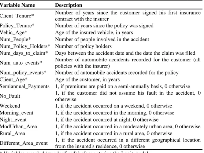
In what concerns the variables used in the model, names and descriptions are described in the following table. One should note, however, that not all of the variables described in the previous section were available, mainly due to missing information for most claims.
Variable Name Description
Client_Tenure* Number of years since the customer signed his first insurance contract with the insurer
Policy_Tenure* Number of years since the policy was signed Vehic_Age* Age of the insured vehicle, in years
Num_People* Number of people involved in the accident Num_Policy_Holders* Number of policy holders
Num_days_to_claim* Days between the accident date and the date the claim was filed Num_auto_events* Number of automobile accidents recorded for the customer (all
policies with the insurer)
Num_policy_events* Number of automobile accidents recorded for the policy Client_Age* Age of the customer, in years
Semiannual_Payments 1, if premiums are paid on a semi-annually basis, 0 otherwise No_Fault 1, if the customer did not assume his fault in the accident, 0
otherwise
Weekend 1, if the accident occurred on a weekend, 0 otherwise Morning_event 1, if the accident occurred in the morning, 0 otherwise Night_event 1, if the accident occurred at night, 0 otherwise
ModUrban_Area 1, if the accident occurred in a moderately urban area, 0 otherwise Rural_Area 1, if the accident occurred in a rural area, 0 otherwise
Different_Area_event 1, if the accident occurred in a different geographical location from the insured's residence, 0 otherwise
* Variables rescaled (standardized) before entering the Logit model.
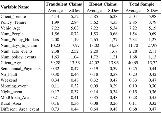
Summary statistics are calculated for the presented variables and shown in the following table. These statistics were computed in relation to the target variable Fraud. One should
15 note that, even for variables that were to be rescaled later in the process, statistics presented here refer to the used sample of 380 claims, using variables in their original state.
Variable Name Fraudulent Claims Honest Claims Total Sample
Average StDev Average StDev Average StDev
Client_Tenure 4,14 5,52 5,85 6,28 5,04 5,98 Policy_Tenure 1,99 2,84 3,62 4,33 2,85 3,79 Vehic_Age 7,22 5,03 7,22 5,34 7,22 5,19 Num_People 1,56 0,72 1,53 0,66 1,54 0,69 Num_Policy_Holders 2,00 1,19 2,65 1,27 2,34 1,27 Num_days_to_claim 10,23 17,97 13,02 34,58 11,70 27,97 Num_auto_events 2,38 2,52 2,20 1,67 2,28 2,11 Num_policy_events 1,63 1,04 1,72 1,21 1,68 1,13 Client_Age 39,28 13,36 42,02 13,96 40,69 13,72 Semiannual_Payments 0,32 0,47 0,19 0,39 0,25 0,44 No_Fault 0,30 0,46 0,18 0,38 0,23 0,42 Weekend 0,34 0,48 0,32 0,47 0,33 0,47 Morning_event 0,11 0,32 0,09 0,29 0,10 0,30 Night_event 0,17 0,37 0,14 0,34 0,15 0,36 ModUrban_Area 0,21 0,41 0,35 0,48 0,28 0,45 Rural_Area 0,16 0,36 0,08 0,26 0,11 0,32 Different_Area_event 0,73 0,44 0,64 0,48 0,68 0,47
These differences will be further analyzed in the results section, concerning their impact in the resulting models.
16
4. Tools and Techniques
Data Mining MethodologyThe use of data mining techniques and methodologies to extract meaningful information from large information systems has been widely accepted, as proven by the extensive literature discussed above. To quote only one other, Smith et al. (2000) has stated that:
Data mining has proven to be a useful approach for attacking this [insurance claim patterns] suite of problems. Each of the sub problems required a different technique and approach, yet the methodology of data mining discussed (…) provided for a logical fusion of the analysis. Rather than using a single technique for solving a single problem, data mining provides a collection of techniques and approaches that help to fully integrate the solutions with existing business knowledge and implementation.
The purpose of this exercise is not, however, to have a mathematical model provide a definite decision about a claim being fraudulent, but rather to estimate a level of similarity between that claim and others that were identified as fraudulent. The recommended decision is then whether to investigate such claim or not. As referenced by Caudill et al. (2005), using a scoring method to identify fraudulent claims can be useful when implementing a claim auditing strategy.
To best take advantage of existing technology when detecting automobile insurance fraud, we selected the software package SPSS Modeler to perform all techniques that might help us identify the most contributing factors and build models, through which one might estimate a fraud propensity for any given claim, given a set of its characteristics.
SPSS Modeler
All statistic procedures included in this work were conducted using SPSS Modeler. SPSS Modeler is a window based software package that enables the use of basic and advanced statistical procedures and common data mining features, beyond those depicted in this thesis.
17 Work in SPSS Modeler is conducted through a process flow diagram designed by the user, selecting which techniques to use from a list of predefined nodes. Many variants are available for each technique, and careful consideration should be employed to navigate all the options presented.
Logistic Regression – Model Definition
For the purpose of automobile insurance fraud, let us define a logistic regression model to explain , which represents the incentive (or utility, in economic terms) of the insured to commit fraud, in any claim . Since logistic models are usually defined in a latent variable context (Artís et al. (2002)), it seems adequate that is unobservable. Nevertheless, one can define the regression model:
(1)
In the presented model, is the vector of explanatory variables, in this model weighted by vector of the unknown regression parameters. is a residual term.
In insurance claim datasets, one cannot observe the utility of the insured when committing fraud. The only available information is dichotomous: whether the claim was identified as fraudulent or honest. This information can be stored in variable , defined as follows:
, if
, otherwise.
Assuming that there is no undetected fraud, the probability of fraud can be derived, using (1), in the following manner:
18
Which, by letting F be the cumulative distribution function of the residual term , means:
(2)
Please note that the absence of undetected fraud is a simplification taken in this thesis and not a pre-requisite of this kind of analysis. Artís et al. (2002), among others, have considered the possibility of misclassification in the response variable, covering the matter in their studies.
In order to estimate the parameter vector , one can use the maximum likelihood method through the maximization of the log-likelihood function. The generic method will not be derived in this thesis but allows the reader to arrive at the following equation, by assuming the residual term above follows a logistic distribution:
(3)
Thus, and once parameters are estimated, equation (3) enables the user to assign, through a set of assumptions, a probability-like score that a claim is fraudulent, given its characteristics .
Classification and Regression Trees – CHAID – Model Definition
An alternative procedure that may provide answers to the issue of predicting insurance fraud is the use of Classification and Regression Trees. Also known as segmentation trees, decision trees or recursive partitioning, C&R Trees have been used frequently as both exploratory tools, as well as predictive tools (Ritschard (2010)).
For the purpose of this thesis, the CHAID variation of C&R Trees will be used. CHAID means Chi-square Automatic Interaction Detector, which, according to Ritschard (2010), is one of the most popular supervised tree growing techniques.
19 The implementation of a model based on a CHAID Tree was first suggested in Kass (1980), and follows a specific algorithm, consisting of 3 global steps: Merging, Splitting and Stopping. The C&R tree grows by repeatedly applying the following algorithm, starting from the root node, i.e., the complete dataset on which it is used (or the full training sample, as we will see in the results section).
Globally, the algorithm will determine the best split for each potential predictor and then select the predictor whose split presents the most significant differences in sub-populations of the training sample, i.e., the lowest p-value for the chi-squared significance test.
Each of these steps will now be described in further detail:
1. Merging
The first part of the algorithm consists of grouping categories in the predictor, or independent, variables. If a predictor is categorical, this part of the algorithm will merge non-significant categories, i.e., any two categories that show the most similar distribution, when compared to the target variable (fraud). The most similar distribution is found by comparing p-values of the Pearson's chi-squared test.
For ordinal predictor, the same method will apply, but only adjacent categories can be merged. Numerical predictors are grouped into exclusive and exhaustive ordinal variables and then treated as such.
The outcome of this step is the identification, for each predictor, of the optimal way to merge categories of that predictor, as well as the optimal p-value for that predictor.
2. Splitting
Taking the outcome of the first part as input, this part of the algorithm will simply select the predictor with the smallest p-value in relation to the target variable. If the p-value is considered significant by the user, i.e. below a significance threshold defined by the user (in this case 5%), the tree is split using that predictor, with merged categories. Otherwise, the node is considered terminal and no split is performed.
20 When a new split is performed, the process restarts at the merging step, for each of the new nodes.
3. Stopping
For each node of the tree, the last part of the algorithm evaluates a set of stopping criteria. The node will not be split if, and only if, any of the following occurs:
a) All records in that node have the same value in the target variable;
b) All predictors have the same value for all records in that node;
c) The maximum number of consecutive splits (tree depth), as defined by the user, has been reached;
d) The number of records in the node is lower than a user-specified minimum;
e) The selected split will create at least one node with a number of records lower than a user-specified minimum.
When no other splits can be performed for any node in the tree, the tree growing algorithm finishes.
Model Accuracy and Performance
All predictive models must be evaluated in terms of accuracy and performance. In other models such as econometric ones, where most predicted variables are quantitative and continuous, model evaluation is performed by measuring the difference between the observed and the predicted values. The probability of a claim being fraudulent, however, is unobservable. Since the only observable variable in this context is the claim’s real classification as fraudulent or legitimate, the model must classify each claim accordingly, assigning a user-defined cut-off point to convert the score calculated in the previous section into a binary variable: fraudulent or honest.
According to Derrig & Francis (2005), it is common for the cut-off point to be 0.5. This means that claims with scores higher than 0.5 will be classified as fraud, while the
21 remaining claims will be predicted to be legitimate. However, one can select different cut-off points for each model. In fact, the selected cut-cut-off point should represent, as reminded by Viaene (2002), the misclassification costs. For the purpose of this thesis, however, the cost of predicting fraud for a legitimate claim is assumed to be the same as that of allowing a fraudulent claim to be indemnified.
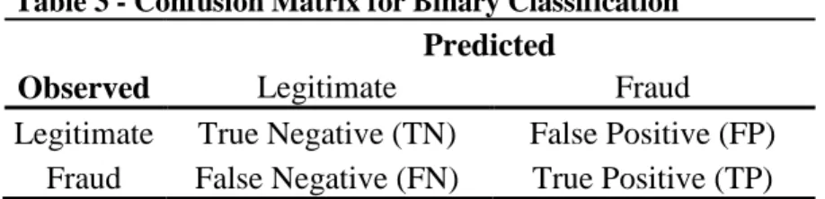
Viaene (2002) suggests that the most used evaluation and comparison statistic is the PCC, percentage correctly classified. PCC, along with other descriptive statistics, such as false positives, false negatives, sensitivity and specificity are the most often used to evaluate and compare model accuracy and predictive power. These can be calculated by defining a so-called Confusion Matrix that combines the four possible outcomes when comparing the predicted classification with the observed one.
Table 3 - Confusion Matrix for Binary Classification
Predicted
Observed Legitimate Fraud
Legitimate True Negative (TN) False Positive (FP) Fraud False Negative (FN) True Positive (TP)
Sensitivity is the percentage of fraudulent claims that were predicted to be fraudulent. On the other hand, specificity is the proportion of legitimate claims predicted to be legitimate. Good models will tend to show high values for these statistics. When both sensitivity and specificity equal 1, the model is considered to be a perfect predictor in the dataset it was used.
Despite being useful statistics to evaluate model accuracy, sensitivity and specificity vary depending on the selected cut-off point. Thus, it is common to plot the two statistics over the range of selectable cut-off points. The most frequently used example of this technique is the receiver operating characteristic (ROC) curve.
22 The ROC curve plots the pairs (sensitivity; 1 – specificity) computed for each cut-off point, allowing a graphical comparison of the overall accuracy of the model. ROC analysis may enable the following interpretation: Since model A’s sensitivity is higher than model B’s,
for all levels of specificity, one can conclude that A usually performs more accurately than B, in the referenced dataset.
ROC analysis, in general, may suffice to provide intuitive or informal model comparison, in terms of accuracy. However, like any graphical comparison, it may prove difficult to rank models whose ROC curves intersect, posing no direct dominance over one another. To overcome this limitation, one often computes the so-called AUROC, literally the area under the ROC curve. Models with higher AUROC are generally considered more accurate.
One important matter must be addressed before the model is generated and the performance indicators are calculated. As part of the data mining methodology, it is recommended to divide the available dataset, i.e. to partition the data in a training sample and a test sample. While the training sample is used to generate the model, its performance is usually best evaluated in the test sample, a set of different claims not used in the building process.
23
5. Results
Logistic RegressionThis section is focused on the application of theory presented in the previous section to the available dataset, further investigating the issue of predicting fraudulent claims in the automobile insurance industry.
Model Variables and Coefficients
The following table summarizes the model obtained through the described procedures:
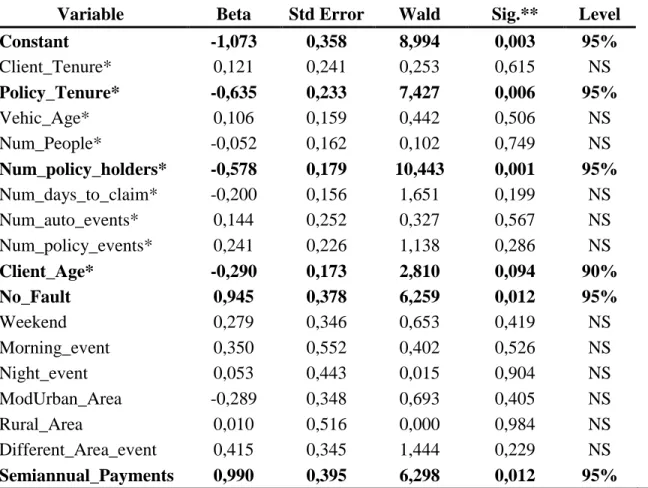
Variable Beta Std Error Wald Sig.** Level
Constant -1,073 0,358 8,994 0,003 95% Client_Tenure* 0,121 0,241 0,253 0,615 NS Policy_Tenure* -0,635 0,233 7,427 0,006 95% Vehic_Age* 0,106 0,159 0,442 0,506 NS Num_People* -0,052 0,162 0,102 0,749 NS Num_policy_holders* -0,578 0,179 10,443 0,001 95% Num_days_to_claim* -0,200 0,156 1,651 0,199 NS Num_auto_events* 0,144 0,252 0,327 0,567 NS Num_policy_events* 0,241 0,226 1,138 0,286 NS Client_Age* -0,290 0,173 2,810 0,094 90% No_Fault 0,945 0,378 6,259 0,012 95% Weekend 0,279 0,346 0,653 0,419 NS Morning_event 0,350 0,552 0,402 0,526 NS Night_event 0,053 0,443 0,015 0,904 NS ModUrban_Area -0,289 0,348 0,693 0,405 NS Rural_Area 0,010 0,516 0,000 0,984 NS Different_Area_event 0,415 0,345 1,444 0,229 NS Semiannual_Payments 0,990 0,395 6,298 0,012 95%
* Variables rescaled (standardized) before entering the Logit model. ** P-values for the Wald test for significance
Policy_Tenure is a significant variable in the model, suggesting that claims related to older insurance policies have a lower probability of being fraudulent. Client_Tenure, however,
24 shows no relevant influence in the outcome. One possible interpretation is that the customer may establish some kind of loyalty towards an insurance company they’ve dealt with for a long time or at least considering a specific insurance policy.
Client_Age has been identified as a significant variable in the model, portraying a tendency for younger people to more likely incur in fraudulent claims. This finding has been observed in other datasets, such as Artís et al. (2002), for instance. However, this variable is only significant at the 10% significance level, so caution is advised when interpreting its coefficient.
The number of policy holders shows a negative influence in the outcome, suggesting that policies signed by a higher number of people are less likely to contain fraudulent claims. One could speculate that a policy holder with intent to commit fraud will probably want to minimize his relationship with the insurer, and therefore avoid providing additional information or sharing ownership of the policy.
In the used dataset, the variable No_Fault has a positive impact on the estimated fraud probability. According to the model, accepting blame in the accident originating the claim increases the chance of the claim being legitimate. This result is contrary to that in Artís et
al. (2002), where it was suggested that, in accepting the blame, claimants of that dataset
might be hoping to reduce the probability of the claim being audited. However, and looking at the model in this thesis, an alternate proposition can be made that fraudulent claimants will not only try to obtain wrongful indemnities but also to do so without incurring in the premium aggravation associated with being blamed for an accident.
The last significant variable identified in the model is Semiannual_Payments. The model suggests that policies with semiannual payments are more likely to contain fraudulent claims, when compared to annual payment policies. This result could indicate that claimants with intent to commit fraud may wish to reduce the initial investment by fractioning premium payments. Alternatively, one could speculate that there is a higher propensity to commit fraud in the lower economic classes of society, but no association
25 between fractioned payment of premiums and policy holder income could be found, so the speculation lacks justification.
Model Accuracy and Performance – LOGIT
As detailed in the previous sections, the most intuitive process to evaluate the accuracy of a classification model is to compare the predicted outcome with the true outcome, and calculate the number of correct predictions. The following confusion matrices summarize the results, for the 0.5 cut-off point:
Training Sample Test Sample
Observed Classification
Predicted Classification Observed Classification
Predicted Classification
Honest Fraud Total Honest Fraud Total
Honest 98 30 128 Honest 52 20 72
Fraud 39 60 99 Fraud 33 48 81
Total 137 90 227 Total 85 68 153
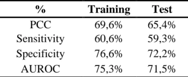
These confusion matrices represent a total PCC of approximately 69.6% for the Training Sample and 65.4% for the Test Sample, as seen in the following table:
% Training Test
PCC 69,6% 65,4%
Sensitivity 60,6% 59,3%
Specificity 76,6% 72,2%
AUROC 75,3% 71,5%
While these results are not the best, other studies have considered similar results to be acceptable (see Artís et al. (2002), for example). The difference between the training sample results and those of the test sample are expected and within normalcy, giving support to saying that the model is not too focused on the specificities of the training sample’s claims (little or no overfitting). The area under the ROC Curve, presented in the previous chapter, is 71.5% for the Test sample, which is commonly considered fair.
Table 5 – Confusion Matrices for the Logit Model - Results
26 As a final note for this section, the following table summarizes the different levels of overall accuracy delivered by the presented model, obtained by selecting different cut-off points for predicting insurance fraud. Additional detail is included in appendix 1:
Cut-Off Threshold
Percentage Correctly Classified (PCC)
Training Sample Test Sample
0% 43,6% 52,9% 10% 46,3% 57,5% 20% 51,5% 60,1% 30% 62,1% 65,4% 40% 67,8% 67,3% 50% 69,6% 65,4% 60% 70,5% 60,1% 70% 68,3% 59,5% 80% 58,1% 50,3% 90% 57,3% 47,7% 100% 56,4% 47,1%
As mentioned, the selected cut-off for the model presented above was 50%: If the score calculated by the model was above this threshold, the claim was predicted to be fraudulent, and legitimate, otherwise. Table 7 indicates that selecting a different cut-off might return more accurate results: selecting 40% would net a 2 point increase in accuracy, for the test sample.
Classification and Regression Trees (CHAID)
As an alternate path to modeling automobile insurance fraud, a classification and regression tree model, using CHAID, was built with the same data set. This section covers the results in further detail.
Model variables and tree design
The CHAID tree selected to predict automobile insurance fraud, with the used dataset is depicted in Table 8 below. As for the technical conditions specified in the model execution,
27 the minimum p-value required for splitting and merging was set to 0.05, with a minimum number of records in parent branch of 20, and a minimum in a child branch of 10.
Additionally, it should be noted that, since the tree growth algorithm treats all variables as either categorical or ordinal, no standardizations were required for this step.
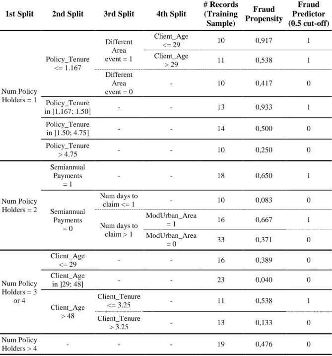
1st Split 2nd Split 3rd Split 4th Split
# Records (Training Sample) Fraud Propensity Fraud Predictor (0.5 cut-off) Num Policy Holders = 1 Policy_Tenure <= 1.167 Different Area event = 1 Client_Age <= 29 10 0,917 1 Client_Age > 29 11 0,538 1 Different Area event = 0 - 10 0,417 0 Policy_Tenure in ]1.167; 1.50] - - 13 0,933 1 Policy_Tenure in ]1.50; 4.75] - - 14 0,500 0 Policy_Tenure > 4.75 - - 10 0,250 0 Num Policy Holders = 2 Semiannual Payments = 1 - - 18 0,650 1 Semiannual Payments = 0 Num days to claim <= 1 - 10 0,083 0 Num days to claim > 1 ModUrban_Area = 1 16 0,667 1 ModUrban_Area = 0 33 0,371 0 Num Policy Holders = 3 or 4 Client_Age <= 29 - - 16 0,389 0 Client_Age in ]29; 48] - - 23 0,040 0 Client_Age > 48 Client_Tenure <= 3.25 - 11 0,538 1 Client_Tenure > 3.25 - 13 0,133 0 Num Policy Holders > 4 - - - 19 0,476 0
28 According to the CHAID model, the number of policy holders in the claim’s policy is the first recommended split that should be applied (p-value of 0.000). This is consistent with what was found in the Logit model, since the number of policy holders significantly contributed to predicting fraud in that model as well. In this dataset, fraudulent claims appear to be differently distributed across 4 categories: 1 policy holder, 2 policy holders, 3 and 4 or more than 4 policy holders, with a higher concentration of fraudulent claims, the lower the number of policy holders (on average). Possible interpretations of this were suggested in the analysis of the Logit model, partly explained by an intention to minimize the relationship with the insurance company, avoiding the involvement of any friends or relatives.
For the second split, three different variables were used, depending on the number of policy holders identified in the first split: the policy’s tenure (p-value 0.001), the flag for indicating semiannual premium payments (0.039) and the client’s age (0.007). All three variables were considered relevant in the Logit model as well.
Concerning policy tenure, for the sub-sample of claims with only one policy holder, it should be noted that the model predicts no fraudulent claims for policies with over 1.5 years of tenure, reassuring the interpretation that a loyalty effect may be in place (as with a negative coefficient in the Logit model).
Concerning semiannual payments, and as suggested by the Logit model, this data set shows a specifically higher concentration of fraudulent claims in policies that share this attribute. The CHAID tree predicts no legitimate claims for this node, and the same interpretation as the one for the Logit model applies: if premeditated fraud is in place, the insured may wish to reduce his/her initial investment but fractioning premium payments.
The last of the second level splits, recommended for policies that have 3 or 4 policy holders, refers to the first policy holder’s age. According to this split, there is a lower concentration of fraudulent claims in the younger policy holders. While this same variable was found to be significant in the Logit model, the interpretations differ. No fraudulent claims are being predicted by the CHAID tree, for claims whose first policy holder is under
29 48 years-old. However, it should be noted that the Logit model does not consider sub-samples of the training data set. Thus, there is no necessary contradiction in this variable and no effects should be ruled out for this reason.
For the third level of splits, and mostly due to the sample size being limited, only three nodes were split, of nine different nodes created by the two earlier splits. These splits revealed significant effects in variables Different Area Event (p-value 0.049), number of days between the accident and the filing of the claim (0.006) and the client’s tenure (0.012). The remaining nodes were considered terminal, as no splits were found for the defined stopping criteria.
Different Area Event, a flag type variable that equals “1” if the accident occurred in a different geographical area from the insurer’s area of residence, is shown to be significant in this specific sub-sample. The CHAID tree suggests that, for fairly recent policies (under 14 months since signing) with only one policy holder, claims tend to be more frequently fraudulent if the accident occurs in a different area than the client’s residence. This can be hypothesized as intent to avoid being recognized, for instance if the accident was simulated or caused intentionally. While this variable was not identified as significant in the Logit model, the same reasoning applies as above, since the CHAID algorithm focuses on different distributions in specific subsamples of the data set. Further to this third level split, an additional split is identified by the tree, distinguishing claims whose client’s age is under or above 29 years (p-value of the fourth level split 0.015). However, this split does not affect the predicted outcome for the selected cut-off, estimating two different propensity levels that still fall on the fraudulent side.
According to the CHAID tree model, not paying premiums semiannually is no reason to rule out possible fraudulent behavior. The model suggests that, if the client takes 2 or more days, after the accident, to file the claim, there may still be a possibility that the claim is fraudulent. In fact, an additional fourth level split is suggested, predicting those claims as fraudulent, if the client lives in a moderately urban area (p-value of the fourth level split 0.033).
30 Lastly, the third level split using the client’s tenure, applicable to policies with 3 or 4 policy holders whose first policy holder is above 48 years of age, suggests different fraud distributions at the 3.25 years of tenure cut-off point. The loyalty effect described above seems to be particularly noticeable above a certain age.
Model Accuracy and Performance – CHAID
In a similar analysis to the one performed for the Logistic Regression model, we now present detailed performance results for the CHAID Classification and Regression defined in the previous section. Unless otherwise stated, all results are for the 50% selected cut-off threshold.
Training Sample Test Sample
Observed Classification
Predicted Classification Observed Classification
Predicted Classification
Honest Fraud Total Honest Fraud Total
Honest 107 21 128 Honest 55 17 72
Fraud 41 58 99 Fraud 35 46 81
Total 148 79 227 Total 90 63 153
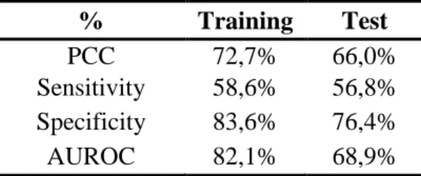
The confusion matrices above represent a Percentage of Correct Classifications of 72.7% for the Training Sample and 66.0% for the Test Sample, as presented below:
% Training Test
PCC 72,7% 66,0%
Sensitivity 58,6% 56,8%
Specificity 83,6% 76,4%
AUROC 82,1% 68,9%
Similarly to the Logit model results, results for the CHAID model are within range of what is commonly considered fair. Comparative results between both models will be further detailed in the following section.
Table 9 – Confusion Matrices for the CHAID Model – Results
31 Concerning the cut-off selection of 0.5, similar to the Logit model, the simulated PCC is as follows:
Cut-Off Threshold
Percentage Correctly Classified (PCC)
Training Sample Test Sample
0% 43,6% 52,9% 10% 58,1% 65,4% 20% 63,0% 65,4% 30% 65,6% 64,7% 40% 71,4% 63,4% 50% 72,7% 66,0% 60% 71,8% 58,2% 70% 66,5% 54,2% 80% 66,5% 54,2% 90% 66,5% 54,2% 100% 56,4% 47,1%
Contrary to the Logit model, and from the presented cut-off points, the 50% cut-off is the one that provides the most accurate results, both for the Training and Test Samples. Additional detail is included in Appendix 2.
Comparative Results between Logit and CHAID
As the final part of this results’ section, we discuss the comparative results between the alternate methodologies applied, in what concerns their accuracy and performance, as well as other aspects.
LOGIT CHAID
50% cut-off Training Test Training Test
PCC 69,6% 65,4% 72,7% 66,0%
Sensitivity 60,6% 59,3% 58,6% 56,8%
Specificity 76,6% 72,2% 83,6% 76,4%
AUROC 75,3% 71,5% 82,1% 68,9%
Table 11 – PCC simulation for different cut-off points in the CHAID Model
32 When comparing performance indicators for both techniques, one might argue that the similarities are greater than the differences. Concerning the PCC, Sensitivity and Specificity indicators, the differences between the Logit and CHAID models can be considered residual, at best. Overall, one could say that there is no relevant difference in accuracy between the two selected models, in this data set, with a slight advantage to the Logit model in terms of Area Under the ROC Curve.
One noticeable difference, however, lies in the loss of accuracy when changing from the Training Sample to the Test Sample. While Logit obtains slightly lower results for the training sample’s PCC, Specificity and AUROC, the decrease that these results show for the test sample is also lower. This is particularly noticeable for the AUROC indicator. While Logit loses 3.8 points, the CHAID value for the test sample is 12.2 points lower than the one for the training sample. One might consider that this difference reveals an abnormal level of over-fitting to the training sample data that might question the model’s use in other datasets.
As a final note, Picture 3 above shows the ROC curves for both models, as approximated by the different cut-off threshold simulations detailed in the previous sections and the
Picture 3 – Comparative ROC Curves: Logit vs CHAID (approximate)
0% 10% 20% 30% 40% 50% 60% 70% 80% 90% 100% 0% 20% 40% 60% 80% 100% S e n si ti v it y 1 - Specificity
Receiving Operating Characteristic (ROC) Curve
(based on Test Sample)
33 matching appendices. As shown, the two curves intercept repeatedly, disallowing a clear recommendation on which model might be preferable.
34
6. Conclusions
The work conducted in this thesis has shown an application of data mining software and techniques in the prediction of automobile insurance fraud.
Using information available in most insurance companies’ databases, in the form of 17 variables that contained characteristics of the policy, the policy holder, the vehicle and the loss event, the Logit model and the CHAID model derived were able to correctly classify 65.4% and 66.0% of claims in the test sample, respectively, which are considered fair results. Each of 380 claims was classified as fraudulent if the probability-like score computed by the models was above 0.5.
In conclusion, the use of the demonstrated tools and techniques enabled the identification of underlying fraud patterns, specific to the raw data used to build the model. Despite the overall accuracy of approximately 66%, key variables were shown to have a significant impact in the outcome of the predicted variable.
The models derived in this thesis suggest a number of “fraud indicators” specific to the used dataset.
Concerning the Logit model, on average, the higher the number of years since the policy was signed, the lower the association with fraudulent claims. The same was true for the number of policy holders. The client’s age was also identified as a significant factor – the average age for the claimant was significantly lower in the population of fraudulent claims than on the legitimate one. Not admitting fault in the accident that led to the claim was also considered an overall suspicious factor, as well as paying premiums semiannually instead of annually.
Concerning the CHAID model, the most significant fraud indicator, and the first split to be applied to the full training sample, was the number of policy holders. Further in the decision tree, and taking into account the sub-populations found after each split, variables such as the policy’s tenure, semiannual payments and the client’s age were considered significant for the second split, allowing very similar interpretations to those of the Logit
35 model. The third and fourth level splits used variables not significant in the Logit model, such as the flag for an accident in a geographical area different from the client’s residential area or the number of days between the accident and the filing of the claim. This has extended the list of possible “fraud indicators” seen in this dataset, even if only applicable to smaller sub-populations.
A comparison of the two derived models was performed, generating very similar performance results between the Logit and CHAID models. Aside from the small difference in the percentage of correctly classified claims, mentioned above, the AUROC indicators differ from 71.5% for the Logit to 68.9% in CHAID.
Perhaps the most noticeable difference is that the tree based algorithm is showing a decrease in AUROC levels from 82.1% in the training sample, to 68.9% in the test sample. This decrease was considered relevant, and suggests some level of over-fitting to the training sample data.
As a final note, the purpose of this work was not solely to present a set of fraud indicators that would help insurance companies target fraudulent behavior in their insurance policies. This thesis aims to present an application of how investing in data mining techniques might be rewarding in the fight against fraudulent behavior. Rather than targeting policies with semiannual payments because it is a significant variable in both models, for instance, companies are encouraged to identify specific fraud indicators in their datasets, taking into account the specificities not found in articles or other academic papers, such as the behavioral patterns of their own clients.
36
7. Limitations and Next Steps
The work developed in this thesis follows a set of assumptions that limits the use of the referred techniques in a real life context, for an insurance company. The following illustrates the limitations of this work.
The first limitation is the assumption that all fraudulent claimants in the dataset are committing the same kind of fraud. This is incurred by working with a binary target variable Fraud that assigns the same value to every kind of fraudulent behavior, and can decrease quality in the results. As in Belhadji et al. (2010), the model is only estimating a probability for a general type of fraud.
While the goal of fraud analysts is to detect any and all kinds of fraud, assigning equal relevance to every kind is a simplification not recommended in a real life application. Suppose, for illustrative purposes, that fraud type A is very frequent among the younger policy holders, while fraud type B is most often perpetrated by the elder: Assigning the same target value to both fraud type A and B will add noise to the model’s characterization of fraudulent claims. In the referred example, there is a possibility that the average age of fraudulent claimants might suggest middle aged people as fraudsters, which, in this example, is not the case.
To deal with this limitation, one could attempt to define various fraud types and assign one to each fraudulent claim. Data mining techniques, such as classification trees or multiple logistical regressions, could then attempt to classify claims as legitimate or fraudulent, for each of the specific fraud types. Additionally, and because there may be fraud types unknown to the user, one is advised to use clustering techniques that may reveal different groups of fraudulent claims, separating, for instance, claimants incurring in fraud type A from those incurring in fraud type B, as above. These alternatives, however, fall beyond the scope of this work, and are suggested for further study.
This thesis is focused in demonstrating the applicability of data mining techniques towards predicting automobile insurance fraud. As mentioned, even if a claim is predicted to be
37 fraudulent, this is not sufficient to save the insurance company from reimbursing the claimant. Taking in consideration that the model assigns a greater fraud probability to specific claims, the insurer may find benefits when choosing to audit those specific claims, instead of purely random ones. This is also referred in Belhadji et al. (2010). However, further applications would need to be conducted in order to estimate and prove these benefits, and a likely subject of further studies.
The last limitation to be depicted in this section, and as in most data mining applications, is the fact that they are intrinsically dependant on the dataset they were applied on. As mentioned in prior chapters, only fraudulent claims that were perceived by the insurance company as fraudulent, and only after an in-depth investigation, were considered
automobile insurance fraud. Each fraudulent claim that the insurer fails to detect will be
adding noise to statistical models in place, and results should always be interpreted cautiously. Moreover, any data mining derived model can only identify fraudulent patterns related to data collected in the adequate time intervals. The more the variables, and the higher their quality, the better any model obtained using the data will tend to become.
38
8. References
Artis, M., Ayuso, M., & Guillén, M., 1999, “Modelling different types of automobile insurance fraud behaviour in the Spanish market”, Insurance: Mathematics and Economics 24 (1999) 67–81
Artis, M., Ayuso, M., & Guillén, M., 2002, “Detection of Automobile Insurance Fraud with Discrete Choice Models and Misclassified Claims”, The Journal of Risk and Insurance, Vol. 69, No. 3 (Sep., 2002)
Belhadji, E., & Dionne, G., 1997, “Development of an Expert System for the Automatic Detection of Automobile Insurance Fraud”, Working paper 97-06, École des Hautes Études Commerciales, Université de Montreal.
Belhadji, E., Dionne, G. & Tarkhani, F., 2000, “A Model for the Detection of Insurance Fraud”, The Geneva Papers on Risk and Insurance 25(4): 517-538.
Bhowmik, R., 2010, “Detecting Auto Insurance Fraud by Data Mining Techniques”,
Journal of Emerging Trends in Computing and Information Sciences, Volume 2 No.4,
APRIL 2011
Caron, L. & Dionne, G., 1998, “Insurance Fraud Estimation: More evidence from the Quebec Automobile Insurance Industry”, Kluwer Academic Publishers, pp 175-182
Caudill, S., Ayuso, M., & Guillén, M., 2005, “Fraud Detection Using a Multinomial Logit Model with Missing Information”, The Journal of Risk and Insurance, Vol. 72, no 4 (2005)
Derrig, R. & Francis, L., 2005, “Comparison of Methods and Software for Modeling Nonlinear Dependencies”, International Congress of Actuaries – Paris – May 28–June 2, 2006
Dionne, G., Giuliano, F. & Picard, P., 2003, “Optimal Auditing for Insurance Fraud”, CIRPEE Working Paper No. 03-29
39 Dugas, C., Bengio, Y., Chapados, N., Vincent, P., Denoncourt, G., & Fournier, C., 2003, “Statistical Learning Algorithms Applied to Automobile Insurance Ratemaking”,
Intelligent Techniques for The Insurance Industry: Theory and Applications, L. Jain et A.F.
Shapiro, editors, World Scientific, 2003.
Elkan, C., 2001, “Magical Thinking in Data Mining: Lessons From CoIL Challenge 2000”,
Proceedings of the seventh ACM SIGKDD international conference on Knowledge discovery and data mining, Pages 426 - 431
Kass, G. V., 1980, “An Exploratory Technique for Investigating Large Quantities of Categorical Data”, Journal of the Royal Statistical Society Series C (Applied Statistics), Vol. 29, No. 2
Kim, H. & Loh, W., 2001, “Classification Trees With Unbiased Multiway Splits”, Journal
of the American Statistical Association, Vol. 96, No. 454 (Jun., 2001), pp. 589-604
Maalouf, T., 2010, “Robust weighted kernel logistic regression in imbalanced and rare events data”, Computational Statistics & Data Analysis; Jan2011, Vol. 55 Issue 1, p168-183, 16p
Pérez, J. M., Muguerza, J., Arbelaitz, O., Gurrutxaga, I., & Martín, J. I., 2005, “Consolidated Tree Classifier Learning in a Car Insurance Fraud Detection Domain with Class Imbalance”, Lecture Notes in Computer Science 3686, Pattern Recognition and Data
Mining. Springer-Verlag. S. Singh et al. (Eds.), 381-389
Phua, C., Lee, V., Smith-Miles, K., Gayler, R., 2010, “A Comprehensive Survey of Data Mining-based Fraud Detection Research”, Computing Research Repository, abs/1009.6119
Quinlan, J. R., 1986, “Induction of Decision Trees”, Machine Learning 1: 81-106, Kluwer Academic Publishers
Ritschard, G., 2010, “CHAID and Earlier Supervised Tree Methods”, Cahiers du
département d’économétrie – Faculté des sciences économiques et sociales - Université de Genève
40 Smith, K. A., Willis, R. J., & Brooks, M., 2000, “An analysis of customer retention and insurance claim patterns using data mining: a case study”, The Journal of the Operational
Research Society, Vol. 51, No. 5 (May, 2000), pp. 532-541
Snider, H., & Tam, S., 1996, “Detecting Fraud With Insurance Data Warehouse”, National
Underwriter, June 1996.
Tennyson, S. & Salsas-Forn, P., 2002, “Claims Auditing in Automobile Insurance - Fraud Detection and Deterrence Objectives”, The Journal of Risk and Insurance, Vol. 69, No. 3 (Sep., 2002), pp. 289-308
Viaene, S., 2002, “A Comparison Of State-Of-The-Art Classification Techniques For Expert Automobile Insurance Claim Fraud Detection”, The Journal of Risk and Insurance, Vol. 69, No. 3 (Sep., 2002), pp. 373-421
Wilson, J. H., 2005, “An Analytical Approach To Detecting Insurance Fraud Using Logistic Regression”, Journal of Finance & Accountancy
41
9. Appendix
Logistic Regression Model Accuracy Results, by selected Cut-Off threshold
Training Sample Selected Cut-Off Point # Predicted Fraud Claims True Positives True Negatives False Positives False
Negatives Sensitivity Specificity PCC
0% 227 99 0 128 0 100% 0% 43,6% 10% 217 97 8 120 2 98% 6% 46,3% 20% 189 89 28 100 10 90% 22% 51,5% 30% 153 83 58 70 16 84% 45% 62,1% 40% 126 76 78 50 23 77% 61% 67,8% 50% 90 60 98 30 39 61% 77% 69,6% 60% 64 48 112 16 51 48% 88% 70,5% 70% 33 30 125 3 69 30% 98% 68,3% 80% 4 4 128 0 95 4% 100% 58,1% 90% 2 2 128 0 97 2% 100% 57,3% 100% 0 0 128 0 99 0% 100% 56,4% Test Sample Selected Cut-Off Point # Predicted Fraud Claims True Positives True Negatives False Positives False
Negatives Sensitivity Specificity PCC
0% 153 81 0 72 0 100% 0% 52,9% 10% 146 81 7 65 0 100% 10% 57,5% 20% 130 75 17 55 6 93% 24% 60,1% 30% 114 71 29 43 10 88% 40% 65,4% 40% 89 60 43 29 21 74% 60% 67,3% 50% 68 48 52 20 33 59% 72% 65,4% 60% 52 36 56 16 45 44% 78% 60,1% 70% 33 26 65 7 55 32% 90% 59,5% 80% 11 8 69 3 73 10% 96% 50,3% 90% 3 2 71 1 79 2% 99% 47,7% 100% 0 0 72 0 81 0% 100% 47,1%
42
CHAID Tree Model Accuracy Results, by selected Cut-Off threshold
Training Sample Selected Cut-Off Point # Predicted Fraud Claims True Positives True Negatives False Positives False
Negatives Sensitivity Specificity PCC
0% 227 99 0 128 0 100% 0% 43,6% 10% 194 99 33 95 0 100% 26% 58,1% 20% 181 98 45 83 1 99% 35% 63,0% 30% 171 96 53 75 3 97% 41% 65,6% 40% 122 78 84 44 21 79% 66% 71,4% 50% 79 58 107 21 41 59% 84% 72,7% 60% 57 46 117 11 53 46% 91% 71,8% 70% 23 23 128 0 76 23% 100% 66,5% 80% 23 23 128 0 76 23% 100% 66,5% 90% 23 23 128 0 76 23% 100% 66,5% 100% 0 0 128 0 99 0% 100% 56,4% Test Sample Selected Cut-Off Point # Predicted Fraud Claims True Positives True Negatives False Positives False
Negatives Sensitivity Specificity PCC
0% 153 81 0 72 0 100% 0% 52,9% 10% 126 77 23 49 4 95% 32% 65,4% 20% 116 72 28 44 9 89% 39% 65,4% 30% 113 70 29 43 11 86% 40% 64,7% 40% 91 58 39 33 23 72% 54% 63,4% 50% 63 46 55 17 35 57% 76% 66,0% 60% 47 32 57 15 49 40% 79% 58,2% 70% 15 13 70 2 68 16% 97% 54,2% 80% 15 13 70 2 68 16% 97% 54,2% 90% 15 13 70 2 68 16% 97% 54,2% 100% 0 0 72 0 81 0% 100% 47,1%
43
CHAID and Exhaustive CHAID Algorithm, as performed in SPSS Modeler®
The CHAID algorithm is originally proposed by Kass (1980) and the Exhaustive CHAID is by Biggs et al (1991). Algorithm CHAID and Exhaustive CHAID allow multiple splits of a node.
Both CHAID and exhaustive CHAID algorithms consist of three steps: merging, splitting
and stopping. A tree is grown by repeatedly using these three steps on each node starting
from the root node.
Merging
For each predictor variable X, merge non-significant categories. Each final category of X will result in one child node if X is used to split the node. The merging step also calculates the adjusted p-value that is to be used in the splitting step.
1. If X has 1 category only, stop and set the adjusted p-value to be 1.
2. If X has 2 categories, go to step 8.
3. Else, find the allowable pair of categories of X (an allowable pair of categories for ordinal predictor is two adjacent categories, and for nominal predictor is any two categories) that is least significantly different (i.e., most similar). The most similar pair is the pair whose test statistic gives the largest p-value with respect to the dependent variable Y. How to calculate p-value under various situations will be described in later sections.
4. For the pair having the largest p-value, check if its p-value is larger than a user-specified alpha-level α merge . If it does, this pair is merged into a single compound category. Then a new set of categories of X is formed. If it does not, then go to step 7.
5. (Optional) If the newly formed compound category consists of three or more original categories, then find the best binary split within the compound category which p-value is the smallest. Perform this binary split if its p-value is not larger than an alpha-levelα split-merge .