A 31P MR spectroscopy study on rat models of liver disease

Universidade de Lisboa

Faculdade de Ciências

Departamento de Física

A 3 1 P M R S p e c t r o s c o p y S t u d y o n

R a t M o d e l s o f L i v e r D i s e a s e

Dissertação

Mestrado Integrado em Engenharia Biomédica e Biofísica

Perfil de Radiacões em Diagnóstico e Terapia

Universidade de Lisboa

Faculdade de Ciências

Departamento de Física

A 3 1 P M R S p e c t r o s c o p y S t u d y o n

R a t M o d e l s o f L i v e r D i s e a s e

Dissertação

Mestrado Integrado em Engenharia Biomédica e Biofísica

Perfil de Radiacões em Diagnóstico e Terapia

Orientador externo: Professor Doutor Maurits Jansen

Orientador interno: Professor Doutor Hugo Ferreira

i |

Table of Contents

1. INTRODUCTION ... 1

1.1 AIM OF THE WORK ... 1

1.2 DISSERTATION OUTLINE ... 2

2. BACKGROUND IN MAGNETIC RESONANCE IMAGING ... 4

2.1 NUCLEAR MAGNETIC RESONANCE ... 4

2.2 RELAXATION PROCESSES AND THE BLOCH EQUATIONS ... 5

2.2.1 Longitudinal Relaxation (T1) ... 5

2.2.2 Transverse Relaxation (T2) ... 5

2.3 CHEMICAL SHIFT ... 6

2.4 SPIN–SPIN COUPLING ... 7

2.5 B1INHOMOGENEITY AND MAPPING B1 TRANSMIT FIELDS ... 9

1.6.1 Double Angle (ratio method) ... 10

2.6 ALTERNATIVE NUCLEI ... 11

2.6.1 Phosphorous 31 ... 11

2.6.2 Identification of Resonances ... 12

3. ANIMAL MODELS OF LIVER FIBROSIS ... 14

3.1 IN-VIVO STUDY ... 15

4. MR SETUP ... 17

4.1 THE MRI APPARATUS ... 17

4.2 MAGNET AND GRADIENT ... 17

4.3 RFCOIL ... 17

4.3.1 Tuning and Matching ... 20

4.4 IN VIVO SPECIFIC HARDWARE ... 21

5. MR SPECTROSCOPY SEQUENCES ... 23

5.1 IMAGE SELECTED IN VIVO SPECTROSCOPY (ISIS) ... 23

5.2 SINGLE PULSE AND 1D ACQUIRE (SPULS) ... 26

5.3 SATURATED SINGLE PULSE (SATSP) ... 27

5.4 CHEMICAL SHIFT IMAGING (CSI) ... 28

5.5 GRADIENT ECHO (GEMS) ... 29

6. EXPERIMENTAL PROTOCOLS ... 30

6.1 PHANTOM PROTOCOL ... 30

6.2 IN VIVO PROTOCOL ... 31

7. METHODS OF DATA ANALYSIS ... 33

7.1 PREPARATION ... 33

7.2 QUANTIFICATION ... 36

7.2.1 AMARES ... 37

8. PHANTOM DESIGN ... 40

8.1 LIVER PHANTOM ... 40

8.1.1 Concept and early draft ... 40

ii |

8.1.3 Phosphorous Components ... 45

8.1.4 Problems and possible solutions ... 47

8.2 PPAPHANTOM ... 49

8.2.1 Phosphorous Components ... 50

8.3 FLIPMAP PHANTOM ... 50

8.3.1 Phosphorous components... 51

9. PHANTOM DATA RESULTS ... 52

9.1 ISIS ... 52

9.2 SPULS ... 53

9.3 SATSP ... 54

9.4 CHEMICAL SHIFT IMAGING ... 56

9.5 PHANTOM DATA ANALYSIS ... 57

10. IN VIVO DATA RESULTS ... 62

10.1 ISIS ... 62

10.2 SATSP ... 63

10.3 CHEMICAL SHIFT IMAGING ... 65

10.4 IN VIVO DATA ANALYSIS ... 69

11. ADDITIONAL RESULTS... 72 11.1 ABSOLUTE QUANTIFICATION ... 72 11.1.1 Discussion ... 75 11.2 B1MAPPING ... 77 11.2.1 Experimental Setup ... 77 11.2.2 Experimental Data ... 77

11.2.3 B1 Map creation (Matlab Script) ... 78

11.2.4 Generated B1 maps ... 79

12. GENERAL DISCUSSION ... 82

13. CONCLUSION ... 85

14. APPENDIX ... 86

14.1SATSP PULSE SEQUENCE ... 86

14.2FLIP ANGLE MAP GENERATION IN MATLAB ... 88

iv |

FIG 1SPIN-SPIN INTERACTIONS INVOLVED WITH SCALAR COUPLING.. ... 8

FIG 2SPIN SPIN COUPLING IN ,1,2-TRICHLOROETHANE DURING 1HMRSPECTROSCOPY. ... 9

FIG 3TYPICAL LOCALIZED IN VIVO 31PNMR SPECTRA FROM (A) RAT SKELETAL MUSCLE,(B) BRAIN AND (C) LIVE. ... 12

FIG 4A TYPICAL SPRAGUE-DAWLEY ALBINOLABORATORYRAT ... 16

FIG 5DOTY SCIENTIFIC DOTY30 ... 18

FIG 6REMOTE COIL MATCHING UNITS, FOR BOTH PROTON AND PHOSPHOROUS, FROM LEFT TO RIGHT. ... 19

FIG 7 REARSIDE VIEW OF THE MAGNET HOLE AND A SCHEMATIC OF VARIAN’S HIGH BAND RF PRE AMPLIFIER. ... 19

FIG 8TUNE INTERFACE BOX AND RE-ROUTING UNIT REPRESENTATIONS, FROM LEFT TO RIGHT. ... 20

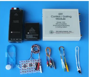
FIG 9 SAINSTRUMENTS INC.(SAII)MODEL 1025MR-COMPATIBLE MONITORING AND GATING SYSTEM. ... 21

FIG 10ISIS PULSE PROGRAM, AS SEEN IN VNMRJ ... 23

FIG 11PULSE SEQUENCE FOR ISIS LOCALIZATION... 24

FIG 12EXPERIMENTAL EVALUATION OF 2DISIS LOCALIZATION BY MRI ... 25

FIG 13SPULS PULSE PROGRAM, AS SEEN IN VNMRJ ... 26

FIG 14SATSP PULSE PROGRAM, AS SEEN IN VNMRJ ... 27

FIG 15CSI PULSE PROGRAM, AS SEEN IN VNMRJ ... 28

FIG 16CSI MAP AND RELATIVE ANATOMICAL REPRESENTATION. ... 28

FIG 17GEMS PULSE PROGRAM, AS SEEN IN VNMRJ ... 29

FIG 18GENERAL VIEW OF JMRUI.ACSI SEQUENCE IS DISPLAYED ... 33

FIG 19APODIZATION TOOLBOX AND ITS EFFECT ON THE VISUAL REPRESENTATION OF A SPECTRUM ... 34

FIG 20PHASING TOOLBOX, SHOWING BOTH ZERO ORDER PHASE AND BEGIN TIME AS FLEXIBLE PARAMETERS. ... 35

FIG 21ZERO FILLING TOOLBOX, WITH THE NUMBER OF POINTS TO ADD TO THE SPECTRUM. ... 35

FIG 22EFFECT OF ZERO FILLING ON SPECTRAL RESOLUTION ... 36

FIG 23A THREE WAY VIEW OF THE AMARES TOOLBOX AS PRESENTED IN JMRUI ... 37

FIG 24EXAMPLE OF GOOD DATA FITTING USING AMARES.ESTIMATED SPECTRUM LOOKS SIMILAR TO THE ORIGINAL ONE. .... 38

FIG 25EXAMPLE OF BAD DATA FITTING USING AMARES.ESTIMATED SPECTRUM BARELY RESEMBLES THE ORIGINAL. ... 38

FIG 26EARLY DRAFT OF THE LIVER PHANTOM ... 40

FIG 27FIRST TRIDIMENSIONAL DRAFT OF THE LIVER PHANTOM ... 41

FIG 28LEFT:TRIDIMENSIONAL MODEL OF THE LIVER PHANTOM.RIGHT:FINAL, PRINTED VERSION OF THE LIVER PHANTOM. 42 FIG 29THREE-WAY PERSPECTIVE OF THE SEPARATED SMALL MPARTMENT, AFTER THE EPOXY RESIN HAD BEEN APPLIED. ... 43

FIG 30THREE-WAY VIEW OF THE COMBINED LARGE AND SMALL COMPARTMENT. ... 44

FIG 31FINAL, DEVELOPED FORM OF THE LIVER PHANTOM ... 45

FIG 32SCOUT IMAGES OF A TRANSVERSAL CUT OF THE LIVER PHANTOM WITH (RIGHT) WITHOUT (LEFT) THE AIR BUBBLE ... 47

FIG 33PPAPHANTOM IN THREE DIFFERENT PERSPECTIVES. ... 49

FIG 34THREEWAY VIEW OF THE FLIPMAP PHANTOM. ... 50

FIG 35ISIS PULSE SEQUENCE |TR2000 MS |256 AVERAGES |25X43X5 MM VOXEL, POSITIONED INSIDE THE SECOND COMPARTMENT |EP[HARD,90°,50 µS,41 DB]|IP[HS-AFP,270°,500 µS,45DB]|VERY HIGH APODIZATION 52 FIG 36ISIS PULSE SEQUENCE |TR2000 MS |256 AVERAGES |25X43X5 MM VOXEL, POSITIONED INSIDE THE SECOND COMPARTMENT |EP[HARD,135°,50 µS,45 DB]|IP[HS-AFP,270°,500 µS,45DB]... 52

FIG 37SPULS SEQUENCE WITH A LOW FLIP ANGLE,HARD PULSE 90°[100 µS,35 DB]|16 AVERAGES |TR2000MS | ... 53

FIG 38SPULS SEQUENCE HIGH FLIP ANGLE,HARD PULSE 350°[100 µS,44 DB]|16 AVERAGES |TR2000MS | ... 53

FIG 39SATSP SEQUENCE |EPHARD 350°[100 µS,45 DB]|SATP HS2090°[2000 µS,33DB]|16 AVERAGES |TR 2000MS | ... 54

FIG 40SATSP SEQUENCE |EPHARD 350°[100 µS,45 DB]|SATP SINC 90°[2000 µS,22DB]|16 AVERAGES |TR 2000MS | ... 54

FIG 41SATSP SEQUENCE |EP,HARD 350°[100 µS,45 DB]|SATP, GAUSS 90°[2000 µS,20DB]|16 AVERAGES |TR 2000MS | ... 55

FIG 42SATSP SEQUENCE |EP,HARD 350°[100 µS,45 DB]|SATP,HARD 360°[110 µS,44DB]|16 AVERAGES |TR 2000MS | ... 55

FIG 43CSI SEQUENCE |2 DUMMY SCANS |32 AVERAGES |TR2000MS |DATA MATRIX 8X8|SLICE ORIENTATION – CORONAL,PHASE 1D 40MM,2D 40MM,THICKNESS 40MM |NO SATURATION BANDS WERE USED ... 56

v |

FIG 45DP SIGNAL AMPLITUDE DEPENDING ON FA ... 58

FIG 46PHENYLPHOSPHONIC ACID SIGNAL AMPLITUDE DEPENDING ON FA ... 59

FIG 47SATURATED VS NON SATURATED SPULS ... 60

FIG 48DP/PPA RATIO WITH INCREASING NUMBER OF AVERAGES ... 61

FIG 49ISIS PULSE SEQUENCE |TR2000 MS |256 AVERAGES |25X31X5 MM VOXEL, POSITIONED INSIDE THE LIVER |EP [HARD,200°,100 µS,44 DB]|IP[HS-AFP,260°,500 µS,46DB] ... 62

FIG 50CONTROL GROUP - SUBJECT N1| HIGH FLIP ANGLE 350°[EP[280 µS,39DB]|64 AVERAGES |SW8000HZ | ... 63

FIG 51CONTROL GROUP - SUBJECT N1| HIGH FLIP ANGLE 350°[EP[280 µS,39DB]|64 AVERAGES |SW8000HZ |SP [360°HARD,140 µS,45DB] ... 63

FIG 52CONTROL GROUP - SUBJECT N2| HIGH FLIP ANGLE 350°[EP[280 µS,39DB]|64 AVERAGES |SW8000HZ | ... 64

FIG 53CONTROL GROUP - SUBJECT N2| HIGH FLIP ANGLE 350°[EP[280 µS,39DB]|64 AVERAGES |SW8000HZ |SP [360°HARD,140 µS,45DB] ... 64

FIG 54CONTROL GROUP - SUBJECT N1|CSI SEQUENCE |2 DUMMY SCANS |64 AVERAGES |TR2000MS |DATA MATRIX 8X8|SLICE -PHASE 1D 60MM,2D 60MM,THICKNESS 10MM |NO SATURATION BANDS WERE USED ... 65

FIG 55CONTROL GROUP - SUBJECT N2|CSI SEQUENCE |2 DUMMY SCANS |64 AVERAGES |TR2000MS |DATA MATRIX 8X8|SLICE -PHASE 1D 60MM,2D 60MM,THICKNESS 10MM |NO SATURATION BANDS WERE USED ... 66

FIG 56DISEASE MODEL GROUP - SUBJECT DM1|CSI SEQUENCE |2 DUMMY SCANS |96 AVERAGES |TR2000MS |DATA MATRIX 8X8|SLICE -PHASE 1D 60MM,2D 60MM,THICKNESS 15MM |NO SATURATION BANDS WERE USED ... 67

FIG 57DISEASE MODEL GROUP - SUBJECT DM1|CSI SEQUENCE |2 DUMMY SCANS |96 AVERAGES |TR2000MS |DATA MATRIX 8X8|SLICE -PHASE 1D 60MM,2D 60MM,THICKNESS 15MM |NO SATURATION BANDS WERE USED ... 68

FIG 58RED SQUARES DEPICTS VOXELS WITH HIGHER TOTAL COMBINED ACQUIRED SIGNAL, WHILE BLUE (ALL THE WAY TO TRANSLUCENT BLUE) SQUARES REPRESENTS THOSE WITH LOWER ACQUIRED SIGNAL. ... 72

FIG 59PPAPHANTOM VOXEL LABEL FOR ABSOLUTE QUANTIFICATION. ... 73

FIG 60THREE FLIPMAP PHANTOM GRADIENT ECHO IMAGES ACQUIRED WITH DIFFERENT NUMBER OF AVERAGES.FROM LEFT TO RIGHT, IMAGES WERE ACQUIRED WITH 32,512 AND 1024 AVERAGES, RESPECTIVELY. ... 78

FIG 61THREE FLIPMAP PHANTOM GRADIENT ECHO IMAGES ACQUIRED WITH DIFFERENT FLIP ANGLES.FROM LEFT TO RIGHT, IMAGES WERE ACQUIRED WITH 20,40 AND 80 DEGREES, RESPECTIVELY. ... 78

FIG 62GENERATED B1 MAP WITHOUT THE NOISE CORRECTION ALGORITHM ... 80

FIG 63GENERATED B1 MAP WITH THE NOISE CORRECTION ALGORITHM. ... 80

TABLE 1CHEMICAL SHIFTS OF BIOLOGICALLY RELEVANT 31P-CONTAINING METABOLITES. ... 13

TABLE 2TYPICAL VALUES/SETTINGS USED IN EACH OF THE AMARES REQUIRED PARAMETERS ... 38

TABLE 3DISODIUM PHOSPHATE CHARACTERISTICS AND CHEMICAL REPRESENTATION. ... 45

TABLE 4PHENYLPHOSPHONIC ACID CHARACTERISTICS AND CHEMICAL REPRESENTATION. ... 46

TABLE 5MONOSODIUM PHOSPHATE CHARACTERISTICS AND CHEMICAL REPRESENTATION. ... 51

TABLE 6SUBJECT DM2 ABSOLUTE METABOLITE CONCENTRATION FOR EACH OF THE 9 CONSIDERED VOXELS... 74

1 |

1. Introduction

2 |

4 |

2. Background in Magnetic Resonance Imaging

2.1 Nuclear Magnetic Resonance

𝛾 =

𝑒

2𝑚

𝑇 = 𝑚

× 𝐵

=

𝑑𝐈

5 |

𝑑𝑚

𝑑𝑡

= 𝛾𝑚

× 𝐵

𝜔

= −𝛾𝐵

𝑣

= (

𝜔

2𝜋

) = (

𝛾

2𝜋

) 𝐵

2.2 Relaxation Processes and the Bloch Equations

2.2.1 Longitudinal Relaxation (T1)

𝑑𝑀

𝑑𝑡

=

𝑀

− 𝑀

𝑇

2.2.2 Transverse Relaxation (T2)

6 |

𝑑𝑀

𝑑𝑡

= −

𝑀

𝑇

+ 𝛾𝑀

𝐵

𝑑𝑀

𝑑𝑡

= −

𝑀

𝑇

− 𝛾𝑀

𝐵

1

𝑇

=

1

𝑇

+

𝛾∆𝐵

2

2.3 Chemical Shift

𝑣

ω

𝛾

7 |

𝐵 = 𝐵

(1 − 𝜎)

σ

σ

𝑣 = (

𝛾

2𝜋

) 𝐵

(1 − 𝜎)

δ

𝛿 =

𝑣

− 𝑣

𝑣

× 10

δ

2.4 Spin–Spin Coupling

8 |

Fig 1 Spin-spin interactions involved with scalar coupling. (A) In isolated atoms, the Fermi contact energetically favors an antiparallel orientation between nuclear and electronic spins. (B) In chemical bonds, the Pauli Exclusion Principle demands that the electron spins are in an antiparallel orientation thereby potentially forcing nuclear and electron spins in an energetically higher parallel orientation, depending on the nuclear spin state [14].

9 |

2.5 B1 Inhomogeneity and Mapping B1 transmit fields

10 |

α

α

α

α

1.6.1 Double Angle (ratio method)

α

α

𝑀

= 𝑀

sin(𝛼)

𝑀

= 𝑀

sin(2𝛼)

α

α

α

𝑀

𝑀

=

2 cos(𝛼) sin(𝛼)

sin(𝛼)

𝛼 = cos

₍

𝑀

2 𝑀

)

α

α

11 |

2.6 Alternative Nuclei

12 |

2.6.2 Identification of Resonances

P

α

β

γ

α

β

γ

Metabolite

Chemical Shift (ppm)

Adenosine monophosphate (AMP)

6.33

Adenosine diphosphate (ADP)

α

-7.05

β

-3.09

Adenosine triphosphate (ATP)

α

-7.52

β

-16.26

Fig 3 Typical localized in vivo 31_{P NMR spectra from (A) rat skeletal muscle, (B) brain and (C) liver.}

13 |

γ

-2.48

Dihydroxyacetone phosphate

7.56

Fructuose-6-phosphate

6.64

Glucose-1-phosphate

5.15

Glucose-6-phosphate

7.20

Glycerol-1-phosphate

7.02

Glycerol-3-phosphorylcoline

2.76

Glycerol-3-phosphorylcethanolamine

3.20

Phosphomonoester (PME)

6.90

Phosphodiester (PDE)

2.20

Inorganic Phosphate

5.02

Phosphocreatine

0.00

Phosphoenolpyruvate

2.06

Phosphorylcoline

5.88

Phosphorylethanolamine

6.78

Nicotinamide adenine dinucleotide (NADH)

-8.30

Table 1 Chemical shifts of biologically relevant 31P-containing metabolites in no specific order [4][14][42][43].

14 |

15 |

16 |

17 |

4. MR Setup

4.1 The MRI apparatus

4.2 Magnet and Gradient

18 |

19 |

Fig 6 Remote Coil Matching Units, for both Proton and Phosphorous, from left to right. These units were used to manually adjust both matching and tuning on each coil, without the need to access it directly.

20 |

4.3.1 Tuning and Matching

Fig 8 Tune Interface Box and Re-Routing Unit representations, from left to right. The Tune Interface Box was used to check the tuning for each nuclei, the lower the value on the display, the better. The Re-Routing Unit was used to link the coil to the Preamplifier while connecting it to the Tuner.

21 |

4.4 In Vivo specific hardware

23 |

5. MR Spectroscopy Sequences

5.1 Image Selected In Vivo Spectroscopy (ISIS)

24 |

Fig 11 Pulse sequence for ISIS localization. For 1D ISIS localization, two experiments are required, one with and one without a spatially selective inversion pulse prior to excitation. Subtraction of the two datasets will only give signal from the localized volume. For 3D localization, eight experiments (2 × 2 × 2) are required as shown, whereby the right column indicates the relative receiver phase (+ = 0◦, − = 180°) [14]

25 |

Fig 12 Experimental evaluation of 2D ISIS localization by MRI. (A) Image representation of a water-filled sphere. No spatially selective (in-plane) inversion pulses were executed. (B and C) Images (in absolute value) in which one spatially selective inversion pulse has been executed. The + and− signs correspond to noninverted and inverted areas, respectively. (D) Image of the sphere after the execution of two spatially orthogonal selective inversion pulses. Due to the double inversion in the middle of the sphere, the magnetization resides along the positive longitudinal axis. (E) The localized volume is obtained according to the following add–subtract scheme : (E) = (A) − (B) − (C) + (D).

26 |

5.2 Single Pulse and 1D acquire (SPULS)

27 |

5.3 Saturated Single Pulse (SATSP)

28 |

5.4 Chemical Shift Imaging (CSI)

Fig 15 CSI pulse program, as seen in vNMRj

Fig 16 CSI map and relative anatomical representation. Each voxel represented on the figure (PPA phantom SCOUT acquired image) on the left has a correspondent spectrum on the right, creating a metabolic matrix.

29 |

◦

◦

◦

5.5 Gradient Echo (GEMS)

30 |

6. Experimental Protocols

31 |

33 |

7. Methods of Data Analysis

7.1 Preparation

Fig 18 General view of jMRUI. A CSI sequence is displayed, where we can see the anatomical image and the selected voxel, the correspondent spectrum as well as a Phase Parameters toolbox

34 |

Fig 19 Apodization Toolbox and its effect on the visual representation of a spectrum. No apodization was used on the left spectrum, as evidenced by the apparently erratic variations, and extreme apodization was used on the spectrum on the left, now displaying very smooth lines

35 |

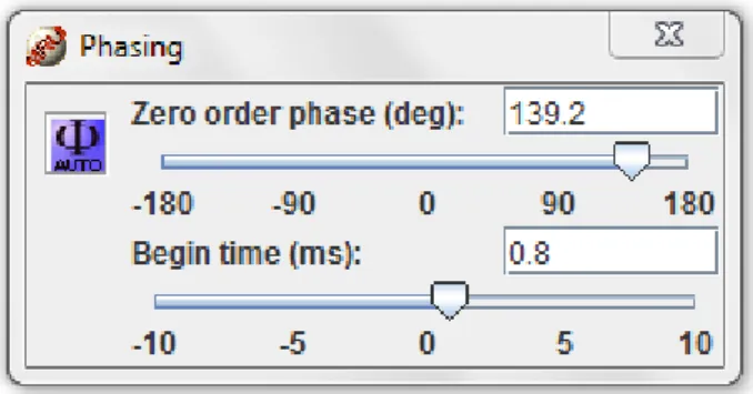
Fig 20 Phasing Toolbox, showing both Zero Order Phase and Begin Time as flexible parameters.

36 |

Fig 22 Effect of zero filling on spectral resolution. The triplet resonance Beta-atp is not well resolved after a FT of the acquired data points. Zero filling the original data (by a power of 2), completely resolves the triplet resonance. After four times zero filling no further improvement in spectral resolution is observed (this, of course, on a case by case basis) [14]

37 |

7.2.1 AMARES

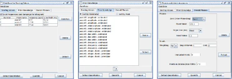
Fig 23 A three way view of the AMARES toolbox as presented in jMRUI, displaying the three main parameter categories at our disposal, “Starting Values”, Prior Knowledge” and “Overall Phases”, from left to right

38 |

Prior Knowledge

Phases

Details

Amplitude Line width Relative

phase Frequency Shape

Zero Order Phase Begin Time Weighting Truncated points Number of Points Estimated Estimated or bound by soft constraints Estimated Estimated or bound by soft constraints Usually Lorentzian Fixed during the analysis of each voxel. Variable between voxels. Fixed On Usually 2 Maximum, dependent on the acquire data set. Table 2 Typical values/settings used in each of the AMARES required parameters

Fig 24 Example of good data fitting using Amares. Estimated spectrum looks similar to the original one.

40 |

8. Phantom Design

8.1 Liver Phantom

8.1.1 Concept and early draft

Fig 26 Early draft of the Liver Phantom. On the left, a sideway cut of both compartments and the surface coil on top. On the right, isometric perspective of the Liver Phantom with the surface coil on top.

41 |

8.1.2 Phantom Design and Production

Fig 27 First tridimensional draft of the Liver Phantom. Both compartments are already in place, design is not final

42 |

Fig 28 Left: Tridimensional model of the Liver Phantom. The two compartments are depicted in different colors for an easier interpretation. Right: Final, printed version of the Liver Phantom. The two pink duplicates are complete. The black phantom is missing its front side, making it possible to see the two separate compartments.

43 |

44 |

45 |

8.1.3 Phosphorous Components

a. Small Compartment (Disodium phosphate)

Table 3 Disodium phosphate characteristics and chemical representation [53].

Molecular

formula

Na

HPO

Molar mass

141.96 g/mol

Appearance

White crystalline solid

Odor

Odorless

Density

1.7 g/cm

Melting point

250 °C

Solubility in

water

7.7 g/100 ml (20 ºC)

Acidity (pKa)

6.83

Fig 31 Final, developed form of the Liver Phantom, next to and positioned inside the small protective plastic container. The container’s cap was itself wrapped in parafilm to supplementary prevent any leaks.

46 |

–

–

b. Large Compartment (Phenylphosphonic Acid)

Molecular

formula

C

HO

P

Molar mass

Appearance

Odor

Odorless

Density

1.422 g/cm

Melting point

163 °C

Solubility in

water

Very soluble

Acidity (pKa)

1.85

Table 4 Phenylphosphonic acid characteristics and chemical representation [53].

–

–

47 |

8.1.4 Problems and possible solutions

Fig 32 SCOUT images of a transversal cut of the Liver Phantom with (right) and without (left) the air bubble (absence of signal in the small compartment),

49 |

8.2 PPA Phantom

50 |

8.2.1 Phosphorous Components

8.3 FlipMap Phantom

51 |

8.3.1 Phosphorous components

Monosodium phosphate

Molecular

formula

NaH2PO4

Molar mass

119.98 g/mol

Appearance

White powder or crystals

Odor

odorless

Density

2.36 g/cm3

Melting point

Solubility in

water

59.9 g/100 mL (0°C)

Acidity (pKa)

4.52

Table 5

–

–

52 |

9. Phantom Data Results

9.1 ISIS

Fig 35 ISIS pulse sequence | TR 2000 ms | 256 averages | 25x43x5 mm voxel, positioned inside the second compartment | EP [Hard, 90°, 50 µs, 41 dB] | IP [HS-AFP, 270°, 500 µs, 45dB] | Very high apodization

Fig 36 ISIS pulse sequence | TR 2000 ms | 256 averages | 25x43x5 mm voxel, positioned inside the second compartment | EP [Hard, 135°, 50 µs, 45 dB] | IP [HS-AFP, 270°, 500 µs, 45dB]

53 |

9.2 SPULS

Fig 37 SPULS sequence with a low flip angle, Hard pulse 90° [100 µs, 35 dB] | 16 averages | TR 2000ms |

54 |

9.3 SATSP

Fig 39 SATSP sequence | EP Hard 350° [100 µs, 45 dB] | SatP hs20 90° [2000 µs, 33dB] | 16 averages | TR 2000ms |

Fig 40 SATSP sequence | EP Hard 350° [100 µs, 45 dB] | SatP sinc 90° [2000 µs, 22dB] | 16 averages | TR 2000ms |

55 |

Fig 41 SATSP sequence | EP, Hard 350° [100 µs, 45 dB] | SatP, gauss 90° [2000 µs, 20dB] | 16 averages | TR 2000ms |

Fig 42 SATSP sequence | EP, Hard 350° [100 µs, 45 dB] | SatP, Hard 360° [110 µs, 44dB] | 16 averages | TR 2000ms |

56 |

9.4 Chemical Shift Imaging

Fig 43 CSI sequence |2 dummy scans | 32 averages | TR 2000ms | Data Matrix 8x8 |Slice orientation – Coronal, Phase 1d 40mm, 2d 40mm, Thickness 40mm |No saturation bands were used

57 |

58 |

Fig 44 Metabolite Ratio varying on applied Flip Angle

Fig 45 DP signal amplitude depending on FA 0,0 20,0 40,0 60,0 80,0 0 50 100 150 200 250 300 350 400 DP/PPA R atio

Flip Angle (degrees)

Metabolite Ratio varying on applied Flip Angle

0 100 200 300 400 500 600 700 0 50 100 150 200 250 300 350 400

Flip Angle (degrees)

59 |

Fig 46 Phenylphosphonic Acid signal amplitude depending on FA 0 20 40 60 80 0 50 100 150 200 250 300 350 400

Flip Angle (degrees)

60 |

Fig 47 Saturated vs Non saturated SPULS 0 5000 10000 15000 20000 25000 0 100 200 300 400 500 600 Peak Am p litu d e Averages

Saturated vs Non saturated SPULS

61 |

Fig 48 DP/PPA ratio with increasing number of averages 0 1 2 3 4 5 6 7 0 100 200 300 400 500 600 D P/PPA R atio Averages

Saturated vs Non-saturated SPULS

62 |

10.

In Vivo Data Results

10.1

ISIS

Control Group [n1]

Fig 49 ISIS pulse sequence | TR 2000 ms | 256 averages | 25x31x5 mm voxel, positioned inside the liver | EP [Hard, 200°, 100 µs, 44 dB] | IP [HS-AFP, 260°, 500 µs, 46dB]

63 |

10.2

SATSP

Control Group [n1]

Fig 51 Control Group - subject n1| high flip angle 350° [EP [280 µs, 39dB] | 64 averages | SW 8000 Hz | SP [360° Hard, 140 µs, 45dB]

64 |

Control Group [n2]

Fig 52 Control Group - subject n2| high flip angle 350° [EP [280 µs, 39dB] | 64 averages | SW 8000 Hz |

Fig 53 Control Group - subject n2| high flip angle 350° [EP [280 µs, 39dB] | 64 averages | SW 8000 Hz | SP [360° Hard, 140 µs, 45dB]

65 |

10.3

Chemical Shift Imaging

Control Group [c1]

Fig 54 Control Group - subject n1 | CSI sequence |2 dummy scans | 64 averages | TR 2000ms | Data Matrix 8x8 |Slice - Phase 1d 60mm, 2d 60mm, Thickness 10mm |No saturation bands were used

66 |

Control Group [c2]

Fig 55 Control Group - subject n2 | CSI sequence |2 dummy scans | 64 averages | TR 2000ms | Data Matrix 8x8 |Slice - Phase 1d 60mm, 2d 60mm, Thickness 10mm |No saturation bands were used

67 |

Disease Model [dm1]

Fig 56 Disease Model group - subject DM1 | CSI sequence |2 dummy scans | 96 averages | TR 2000ms | Data Matrix 8x8 |Slice - Phase 1d 60mm, 2d 60mm, Thickness 15mm |No saturation bands were used

68 |

Disease Model [dm2]

Fig 57 Disease Model group - subject DM1 | CSI sequence |2 dummy scans | 96 averages | TR 2000ms | Data Matrix 8x8 |Slice - Phase 1d 60mm, 2d 60mm, Thickness 15mm |No saturation bands were used

69 |

10.4 In Vivo Data Analysis

70 |

α β

γ

72 |

11. Additional Results

11.1 Absolute Quantification

Fig 58 Red squares depicts voxels with higher total combined acquired signal, while blue (all the way to translucent blue) squares represents those with lower acquired signal.

73 |

Fig 59 PPA Phantom Voxel label for absolute quantification.

74 |

SUBJECT DM2 - ABSOLUTE METABOLITE CONCENTRATION

PPA Test Data

Voxel Amplitude C Voxel Amplitude C Voxel Amplitude C [5,3] 1911 50 [5,4] 2176 50 [5,5] 2186 50 [4,3] 2023 [4,4] 2452 [4,5] 2571 [3,3] 1375 [3,4] 1767 [3,5] 1945 Adjusted C Adjusted C Adjusted C PME Voxel PME Voxel PME Voxel [5,3] 3.3 [5,4] 12.2 [5,5] 10.9 [4,3] 11.8 [4,4] 9.4 [4,5] 18.9 [3,3] 21.3 [3,4] 22.6 [3,5] 19.9 Adjusted C Adjusted C Adjusted C PDE Voxel PDE Voxel PDE Voxel [5,3] 2.8 [5,4] 4.0 [5,5] 6.2 [4,3] 3.9 [4,4] 4.1 [4,5] 5.1 [3,3] 6.3 [3,4] 8.8 [3,5] 6.4 Adjusted C Adjusted C Adjusted C PCr Voxel PCr Voxel PCr Voxel [5,3] 29.0 [5,4] 26.1 [5,5] 15.7 [4,3] 21.2 [4,4] 16.8 [4,5] 10.4 [3,3] 9.6 [3,4] 5.3 [3,5] 2.2 Adjusted C Adjusted C Adjusted C γ-ATP Voxel γ-ATP Voxel γ-ATP Voxel [5,3] 12.1 [5,4] 13.6 [5,5] 13.9 [4,3] 11.8 [4,4] 12.7 [4,5] 11.5 [3,3] 10.6 [3,4] 8.5 [3,5] 8.3 Adjusted C Adjusted C Adjusted C α-ATP Voxel α-ATP Voxel α-ATP Voxel [5,3] 16.1 [5,4] 19.9 [5,5] 19.8 [4,3] 16.6 [4,4] 19.6 [4,5] 18.7 [3,3] 22.8 [3,4] 16.1 [3,5] 13.9 Adjusted C Adjusted C Adjusted C β-ATP Voxel β-ATP Voxel β-ATP Voxel [5,3] 13.3 [5,4] 15.5 [5,5] 16.0 [4,3] 11.5 [4,4] 12.6 [4,5] 12.5 [3,3] 11.1 [3,4] 7.9 [3,5] 8.7

75 |

76 |

𝐶

=

𝑆

𝑆

[𝑚] = (

𝑆

_𝑆

77 |

11.2 B1 Mapping

11.2.1 Experimental Setup

11.2.2 Experimental Data

Flip Angle

(degrees) Averages TR (s) TE (ms) FOV

Slice Thickness (mm) Data Matrix GEMS 20 32 10 4 100x100 2 128x128 20 512 20 40 512 80 512 20 1024 80 1024 40 1024

78 |

11.2.3 B1 Map creation (Matlab Script)

%% Both images, acquired with different flip angles, are %% loaded and converted into doubles. A Flip Angle matrix %% (FA) is defined, having the same size as the previously %% loaded images. This FA matrix will later carry a flip %% angle value for each pixel. doublei40 matrix is created %% as the supposed multiple of matrix i20.

Fig 60 Three FlipMap phantom gradient echo images acquired with different number of averages. From left to right, images were acquired with 32, 512 and 1024 averages, respectively.

Fig 61 Three FlipMap phantom gradient echo images acquired with different flip angles. From left to right, images were acquired with 20, 40 and 80 degrees, respectively.

79 |

i40 = imread('NaP 1024av 40deg.jpg'); i80 = imread('NaP 1024av 80deg.jpg'); i40 = double(i40);

i80 = double(i80); FA = zeros(128,128); doublei40 = 2*i40;

%% A threshold (T) is set for the signal magnitude, below

%% which a specific pixel is considered to be noise.

T = 45; for i = 1:1:128; for j =1:1:128; if doublei40(i,j) < T doublei40(i,j) = 1; end if i80(i,j) < T i40(i,j) = 1; end FA(i,j) = acosd(i80(i,j)/doublei40(i,j)); end end

%% New matrix FAR (Flip Angle Real) cuts out the imaginary %% part of the FA matrix. Then, a noise reducing mechanism %% is applied. FAR = real(FA); for i = 1:1:128; for j =1:1:128; if FAR(i,j) > 80 FAR(i,j) = 1; end end end imagesc(FAR, [20,70]);

For the code to work as intended, the position of the phantom/subject must be

kept exactly the same in relation to the coil, as the algorithm assumes that the

position of each pixel is the same for both acquired images.

80 |

Fig 62 Generated B1 map without the noise correction algorithm

82 |

85 |

86 |

14.

Appendix

14.1 SATSP pulse sequence

1 #ifndef LINT

2 static char SCCSid[] = "modified SPULS/PRESS with saturation bands";

3 #endif 4 /*

5 * Varian,Inc. All Rights Reserved.

6 * This software contains proprietary and confidential

7 * information of Varian, Inc. and its contributors.

8 * Use, disclosure and reproduction is prohibited without

9 * prior consent.

10 */

11 /****************************************************************** 12 SPULS + Saturation Slices

13 14 ******************************************************************/ 15 16 #include <standard.h> 17 #include "sgl.c" 18 19 20 pulsesequence() 21 {

22 /***** Internal variable declarations *****/ 23 double te_d1,te_d2,te_d3; /* delays */

24 double tr_delay;

25 double freq1,freq2,freq3;

26 char volumercv[MAXSTR];

27 28

29 get_parameters();

30 get_ovsparameters();

31

32 initparms_sis(); /* initialize standard imaging parameters */

33

34 getstr("volumercv",volumercv);

35

36 te2 = getvalnwarn("te2");

37

38 /***** RF power calculations *****/ 39 init_rf(&p1_rf,p1pat,p1,flip1,rof1,rof2);

40 init_rf(&p2_rf,p2pat,p2,flip2,rof1,rof2);

41 calc_rf(&p1_rf,"tpwr1","tpwr1f");

42 calc_rf(&p2_rf,"tpwr2","tpwr2f");

43

44 /***** Initialize gradient structs *****/ 45 init_slice(&vox1_grad,"vox1",vox1);

46 init_slice_refocus(&vox1r_grad,"vox1r");

47

48 /***** Gradient calculations *****/

49 calc_slice(&vox1_grad,&p1_rf,WRITE,"gvox1");

50 calc_slice_refocus(&vox1r_grad,&vox1_grad,WRITE,"gvox1r");

51

52 if (vox1_grad.rfDelayFront < 0.2e-6) vox1_grad.rfDelayFront = 0;

53 if (vox1_grad.rfDelayBack < 0.2e-6) vox1_grad.rfDelayBack = 0;

54 55

56 /* Optional Outer Volume Suppression and Saturation Bands */

57 if (ovs[0] == 'y') create_ovsbands();

58 if (sat[0] == 'y') create_satbands();

59

60 /***** Min TR *****/ 61 trmin = 4e-6 + at;

62

63 if (ovs[0] == 'y') trmin += ovsTime;

64 if (sat[0] == 'y') trmin += satTime;

65

66 if (mintr[0] == 'y') {

67 tr = trmin+4e-6; // ensure at least 4us between gradient events

87 |

69 }

70 if (tr < trmin+4e-6) {

71 abort_message("tr too short. Minimum tr = %.2f ms\n",(trmin+4e-6)*1000);

72 } 73 74 /***** Calculate TR delay *****/ 75 tr_delay = tr - trmin; 76 77 78 /* Frequency offsets */

79 freq1 = poffset(pos1,vox1_grad.ssamp); // First RF pulse

80 roff = resto-tof; // receiver frequency, delta from transmitter

81 tof=5500;

82 83

84 /* Put gradient information back into VnmrJ parameters */

85 putvalue("gvox1",vox1_grad.ssamp);

86

87 putvalue("rgvox1",vox1_grad.tramp);

88

89 putvalue("tvox1",vox1r_grad.duration);

90 putvalue("rgvox1r",vox1r_grad.tramp);

91 92 93 sgl_error_check(sglerror); 94 95 96 /* Relaxation delay ***********************************/ 97 status(A); 98 obsoffset(resto); 99 delay(4e-6);

100 rot_angle(vpsi,vphi,vtheta);

101 xgate(ticks);

102

103 if (ix == 1) grad_advance(tep);

104

105 /* Saturation bands ***********************************/

106 if (ovs[0] == 'y') ovsbands();

107 if (sat[0] == 'y') satbands();

108 delay(4e-6);

109

110 /* Slice selective 90 degree RF pulse *****/

111

112 obspower(tpwr);

113

114 shapedpulse(pwpat,pw,oph,rof1,rof2);

115 116 startacq(alfa); 117 acquire(np,(1.0/sw)); 118 endacq(); 119 120 delay(tr_delay); 121 122 }

88 |

14.2 Flip Angle map generation in matlab

1 /* Matlab code for B1 map generation (example) */

2

3 i40 = imread('NaP 1024av 40deg.jpg');

4 i80 = imread('NaP 1024av 80deg.jpg');

5 i40 = double(i40);

6 i80 = double(i80);

7 8 FA = zeros(128,128); 9 T = 45; 10 11 ii40 = 2*i40; 12 13 for i = 1:1:128; 14 for j =1:1:128; 15 16 if ii40(i,j) < T 17 ii40(i,j) = 1; 18 end 19 20 if i80(i,j) < T 21 i80(i,j) = 1; 22 end 23

24 FA(i,j) = acosd(i80(i,j)/ii40(i,j));

25 end 26 end 27 28 FAR = real(FA); 29 for i = 1:1:128; 30 for j =1:1:128; 31 if FAR(i,j) > 80 32 FAR(i,j) = 1; 33 end 34 end 35 end 36 37 imagesc(FAR, [20,70]);

89 |

15. References

[1]

P. Rossi, P. Ricci, and L. Broglia, Portal Hypertension: Diagnostic Imaging and Imaging-guided Therapy ; with 49 Tables. Springer Science & Business Media, 2000.

[2]

R. N. Anderson and B. L. Smith, “Deaths: leading causes for 2001,”Natl Vital Stat Rep, vol. 52, no. 9, pp. 1–85, Nov. 2003. [3]

L. Castéra, J. Vergniol, J. Foucher, B. Le Bail, E. Chanteloup, M. Haaser, M. Darriet, P. Couzigou, and V. De Lédinghen, “Prospective comparison of transient elastography, Fibrotest, APRI, and liver biopsy for the assessment of fibrosis in chronic hepatitis C,”Gastroenterology, vol. 128, no. 2, pp. 343–350, Feb. 2005.

[4]

I. R. Corbin, R. Buist, J. Peeling, M. Zhang, J. Uhanova, and G. Y. Minuk, “Hepatic 31P MRS in rat models of chronic liver disease: assessing the extent and progression of disease,” Gut, vol. 52, no. 7, pp. 1046–1053, Jul. 2003.

[5]

M. Ronot, S. A. Lambert, M. Wagner, P. Garteiser, S. Doblas, M. Albuquerque, V. Paradis, V. Vilgrain, R. Sinkus, and B. E. Van Beers, “Viscoelastic Parameters for Quantifying Liver Fibrosis: Three-Dimensional Multifrequency MR Elastography Study on Thin Liver Rat Slices,” PLoS ONE, vol. 9, no. 4, p. e94679, Apr. 2014.

[6]

H. J. Alter, Y. Nakatsuji, J. Melpolder, J. Wages, R. Wesley, J. W. Shih, and J. P. Kim, “The incidence of transfusion-associated hepatitis G virus infection and its relation to liver disease,” N. Engl. J. Med., vol. 336, no. 11, pp. 747–754, Mar. 1997.

[7]

K. K. Changani, B. J. Fuller, D. J. Bryant, J. D. Bell, M. Ala-Korpela, S. D. Taylor-Robinson, D. P. Moore, and B. R. Davidson, “Non-invasive assessment of ATP regeneration potential of the preserved donor liver. A 31P MRS study in pig liver,” J. Hepatol., vol. 26, no. 2, pp. 336–342, Feb. 1997.

[8]

E. M. Haacke, R. W. Brown, M. R. Thompson, and R. Venkatesan,Magnetic Resonance Imaging: Physical Principles and Sequence

Design, 1st edition. New York: Wiley-Liss, 1999.

[9]

C. Westbrook, C. K. Roth, and J. Talbot, MRI in Practice, 4th Edition edition. Chichester, West Sussex ; Malden, MA: Wiley-Blackwell, 2011.

[10]

M. A. Flower, Webb’s Physics of Medical Imaging, Second Edition. CRC Press, 2012. [11]

V. Kuperman, Magnetic Resonance Imaging: Physical Principles and Applications. Academic Press, 2000. [12]

J. C. Maxwell and F. Jenkin, “LXI. On the elementary relations between electrical measurements,” Philosophical Magazine Series 4, vol. 29, no. 198, pp. 436–460, Jun. 1865.

[13]

F. Bloch, R. I. Condit, and H. H. Staub, “Neutron Polarization and Ferromagnetic Saturation,” Phys. Rev., vol. 70, no. 11–12, pp. 972– 973, Dec. 1946.

[14]

R. A. de Graaf, In Vivo NMR Spectroscopy: Principles and Techniques, 2nd Edition edition. Chichester, West Sussex, England ; Hoboken, NJ: Wiley-Blackwell, 2007.

[15]

Lebon V, Petersen KF, Cline GW, Shen J, Mason GF, Dufour S, Behar KL, Shulman GI, Rothman DL. Astroglial contribution to brain energy metabolism in humans revealed by 13C nuclear magnetic resonance spectroscopy: elucidation of the dominant pathway for neurotransmitter glutamate repletion and measurement of astrocytic oxidative metabolism. J Neurosci 22, 1523–1531 (2002). [16]

Bluml S, Moreno-Torres A, Shic F, Nguy CH, Ross BD. Tricarboxylic acid cycle of glia in the in vivo human brain. NMR Biomed 15, 1– 5 (2002).

[17]

Blakely RD, Coyle JT. The neurobiology of N-acetylaspartylglutamate. Int Rev Neurobiol 30, 39–100 (1988).

[18]

H. Van As and D. van Dusschoten, “NMR methods for imaging of transport processes in micro-porous systems,” Geoderma, vol. 80, no. 3–4, pp. 389–403, Nov. 1997.

90 |

G. R. Morrell, “A phase-sensitive method of flip angle mapping,” Magn. Reson. Med., vol. 60, no. 4, pp. 889–894, Oct. 2008. [20]

C. H. Cunningham, K. S. Nayak, and J. M. Pauly, “RF field mapping for magnetic resonance imaging,” US7446526 B2, 04-Nov-2008. [21]

L. I. Sacolick, F. Wiesinger, I. Hancu, and M. W. Vogel, “B1 Mapping by Bloch-Siegert Shift,” Magn Reson Med, vol. 63, no. 5, pp. 1315–1322, May 2010.

[22]

R. Stollberger and P. Wach, “Imaging of the active B1 field in vivo,”Magn. Reson. Med., vol. 35, no. 2, pp. 246–251, Feb. 1996. [23]

R. Treier, A. Steingoetter, M. Fried, W. Schwizer, and P. Boesiger, “Optimized and combined T1 and B1 mapping technique for fast and accurate T1 quantification in contrast-enhanced abdominal MRI,” Magn. Reson. Med., vol. 57, no. 3, pp. 568–576, Mar. 2007. [24]

“Section 5.5: Spin-spin coupling,” chemwiki.ucdavis.edu. [Online]. Available:

http://chemwiki.ucdavis.edu/Organic_Chemistry/Organic_Chemistry_With_a_Biological_Emphasis/Chapter_05%3A_Structure_De termination_II/Section_5.5%3A_Spin-spin_coupling. [Accessed: 11-Oct-2014].

[25]

R. Issa, X. Zhou, N. Trim, H. Millward-Sadler, S. Krane, C. Benyon, and J. Iredale, “Mutation in collagen-1 that confers resistance to the action of collagenase results in failure of recovery from CCl4-induced liver fibrosis, persistence of activated hepatic stellate cells, and diminished hepatocyte regeneration,” FASEB J, vol. 17, no. 1, pp. 47–49, 2003.

[26]

J. P. Iredale, “Hepatic Stellate Cell Behavior during Resolution of Liver Injury,” Seminars in Liver Disease, vol. 21, no. 03, pp. 427–436, 2001.

[27]

F. Ursini, M. Maiorino, M. Valente, L. Ferri, and C. Gregolin, “Purification from pig liver of a protein which protects liposomes and biomembranes from peroxidative degradation and exhibits glutathione peroxidase activity on phosphatidylcholine hydroperoxides,” Biochimica et Biophysica Acta (BBA) - Lipids and Lipid Metabolism, vol. 710, no. 2, pp. 197–211, Feb. 1982. [28]

Y. Kamada, S. Tamura, S. Kiso, H. Matsumoto, Y. Saji, Y. Yoshida, K. Fukui, N. Maeda, H. Nishizawa, H. Nagaretani, Y. Okamoto, S. Kihara, J. Miyagawa, Y. Shinomura, T. Funahashi, and Y. Matsuzawa, “Enhanced carbon tetrachloride-induced liver fibrosis in mice lacking adiponectin,” Gastroenterology, vol. 125, no. 6, pp. 1796–1807, Dec. 2003.

[29]

G. Vendemiale, I. Grattagliano, M. L. Caruso, G. Serviddio, A. M. Valentini, M. Pirrelli, and E. Altomare, “Increased Oxidative Stress in Dimethylnitrosamine-Induced Liver Fibrosis in the Rat: Effect of N-Acetylcysteine and Interferon-α,” Toxicology and Applied

Pharmacology, vol. 175, no. 2, pp. 130–139, Sep. 2001.

[30]

“Systemic Infusion of FLK1+ Mesenchymal Stem Cells Ameliorate... : Transplantation.” [Online]. Available:http://journals.lww.com/transplantjournal/Fulltext/2004/07150/Systemic_Infusion_of_FLK1__Mesenchymal_Stem_Cell s.14.aspx. [Accessed: 11-Oct-2014].

[31]

C. Constandinou, N. Henderson, and J. P. Iredale, “Modeling Liver Fibrosis in Rodents,” in Fibrosis Research, J. Varga, D. A. Brenner, and S. H. Phan, Eds. Totowa, NJ: Humana Press, 2005, pp. 237–250.

[32]

A. Canbay, S. Friedman, and G. J. Gores, “Apoptosis: The nexus of liver injury and fibrosis,” Hepatology, vol. 39, no. 2, pp. 273–278, Feb. 2004.

[33]

P. Hammel, A. Couvelard, D. O’Toole, A. Ratouis, A. Sauvanet, J. F. Fléjou, C. Degott, J. Belghiti, P. Bernades, D. Valla, P. Ruszniewski, and P. Lévy, “Regression of Liver Fibrosis after Biliary Drainage in Patients with Chronic Pancreatitis and Stenosis of the Common Bile Duct,” New England Journal of Medicine, vol. 344, no. 6, pp. 418–423, Feb. 2001.

[34]

P. de la M Hall, C. S. Lieber, L. M. DeCarli, S. W. French, K. O. Lindros, H. Järveläinen, C. Bode, A. Parlesak, and J. C. Bode, “Models of alcoholic liver disease in rodents: a critical evaluation,” Alcohol. Clin. Exp. Res., vol. 25, no. 5 Suppl ISBRA, p. 254S–261S, May 2001.

[35]

P. P. Simeonova, R. M. Gallucci, T. Hulderman, R. Wilson, C. Kommineni, M. Rao, and M. I. Luster, “The Role of Tumor Necrosis Factor-α in Liver Toxicity, Inflammation, and Fibrosis Induced by Carbon Tetrachloride,” Toxicology and Applied Pharmacology, vol. 177, no. 2, pp. 112–120, Dec. 2001.

91 |

S. Sawada, K. Murakami, J. Murata, K. Tsukada, and I. Saiki, “Accumulation of extracellular matrix in the liver induces high metastatic potential of hepatocellular carcinoma to the lung,” International Journal of Oncology, vol. 19, no. 1, pp. 65–70, Jul. 2001.

[37]

J. A. Fallowfield and J. P. Iredale, “Targeted treatments for cirrhosis,”Expert Opin. Ther. Targets, vol. 8, no. 5, pp. 423–435, Oct. 2004. [38]

Y. N. Kallis, A. J. Robson, J. A. Fallowfield, H. C. Thomas, M. R. Alison, N. A. Wright, R. D. Goldin, J. P. Iredale, and S. J. Forbes, “Remodelling of extracellular matrix is a requirement for the hepatic progenitor cell response,” Gut, vol. 60, no. 4, pp. 525–533, 2011. [39]

J. A. Fallowfield, “Therapeutic targets in liver fibrosis,” American Journal of Physiology - Gastrointestinal and Liver Physiology, vol. 300, no. 5, pp. G709–G715, May 2011.

[40]

A. Pellicoro, P. Ramachandran, J. P. Iredale, and J. A. Fallowfield, “Liver fibrosis and repair: immune regulation of wound healing in a solid organ,” Nat Rev Immunol, vol. 14, no. 3, pp. 181–194, Mar. 2014.

[41]

“Laboratory rat,” Wikipedia, the free encyclopedia. 11-Oct-2014. [42]

O. D. Bengt Noren, “Separation of advanced from mild fibrosis in diffuse liver disease using 31P magnetic resonance spectroscopy” European journal of radiology, vol. 66, no. 2, pp. 313–20, 2008.

[43]

J. D. Bell, I. J. Cox, J. Sargentoni, C. J. Peden, D. K. Menon, C. S. Foster, P. Watanapa, R. A. Iles, and J. Urenjak, “A 31P and 1H-NMR investigation in vitro of normal and abnormal human liver,” Biochim. Biophys. Acta, vol. 1225, no. 1, pp. 71–77, Nov. 1993. [44]

A. Kumar and P. A. Bottomley, “Optimized quadrature surface coil designs,” MAGMA, vol. 21, no. 1–2, pp. 41–52, Mar. 2008. [45]

R. J. Ordidge, A. Connelly, and J. A. B. Lohman, “Image-selected in Vivo spectroscopy (ISIS). A new technique for spatially selective nmr spectroscopy,” Journal of Magnetic Resonance (1969), vol. 66, no. 2, pp. 283–294, Feb. 1986.

[46]

S. S. Rajan, “MRI Hardware System Components,” in MRI, Springer New York, 1998, pp. 25–39. [47]

J. P. Hannon, “Effect of Temperature on the Heart Rate, Electrocardiogram and Certain Myocardial Oxidations of the Rat,”Circulation

Research, vol. 6, no. 6, pp. 771–778, 1958.

[48]

X. He and D. A. Yablonskiy, “Biophysical mechanisms of phase contrast in gradient echo MRI,” PNAS, vol. 106, no. 32, pp. 13558– 13563, 2009.

[49]

Vanhamme, van den Boogaart A, and Van Huffel S, “Improved method for accurate and efficient quantification of MRS data with use of prior knowledge,” J. Magn. Reson., vol. 129, no. 1, pp. 35–43, Nov. 1997.

[50]

J. Weis, L. Johansson, F. Ortiz-Nieto, and H. Ahlström, “Assessment of lipids in skeletal muscle by LCModel and AMARES,” J Magn

Reson Imaging, vol. 30, no. 5, pp. 1124–1129, Nov. 2009.

[51]

D. E. Bohning, A. C. Wright, and K. M. Spicer, “In vivo phosphorus spectroscopy of human skin,” Magn. Reson. Med., vol. 35, no. 2, pp. 186–193, Feb. 1996.

[52]

“Plastic Properties of Acrylonitrile Butadiene Styrene (ABS),” www.dynalabcorp.com [Online]. Available:

http://www.dynalabcorp.com/technical_info_abs.asp. [Accessed: 11-Oct-2014]. [53]

“Chemical Database” www.chemspider.com [Online] [54]

C. J. Cooksey, E. J. Land, and P. A. Riley, “A SIMPLE ONEPOT PREPARATION OF 4ALKOXYAND 4ALKYLTHIOCATECHOLS AND o -BENZOQUINONES,” Organic Preparations and Procedures International, vol. 28, no. 4, pp. 463–467, Aug. 1996.

92 |

K. Schrödter, G. Bettermann, T. Staffel, F. Wahl, T. Klein, and T. Hofmann, “Phosphoric Acid and Phosphates,” in Ullmann’s

Encyclopedia of Industrial Chemistry, Wiley-VCH Verlag GmbH & Co. KGaA, 2000.

[56]

S. Fortune, M. A. Jansen, T. Anderson, G. A. Gray, J. E. Schneider, P. R. Hoskins, and I. Marshall, “Development and characterization of rodent cardiac phantoms: comparison with in vivo cardiac imaging,”Magn Reson Imaging, vol. 30, no. 8, pp. 1186–1191, Oct. 2012.

[57]

G. A. Webb, Modern Magnetic Resonance: Part 1: Applications in Chemistry, Biological and Marine Sciences, Part 2: Applications in

Medical and Pharmaceutical Sciences, Part 3: Applications in Materials Science and Food Science. Springer Science & Business Media,

2007. [58]

“Magnetism,” Questions and Answers in MRI. [Online]. Available:http://mriquestions.com/adiabatic-pulses.html. [Accessed: 03-Dec-2014].

[59]

B. Norén, P. Lundberg, M. Ressner, S. Wirell, S. Almer, and O. Smedby, “Absolute quantification of human liver metabolite concentrations by localized in vivo 31P NMR spectroscopy in diffuse liver disease,” Eur Radiol, vol. 15, no. 1, pp. 148–157, Jan. 2005.