Admission Control based on End-to-end Delay Estimation to Enhance the Support of Real-Time Traffic in Wireless Sensor Networks

M A P

tele

DOCTORAL PROGRAMME IN TELECOMMUNICATIONS

Admission Control based on End-to-end Delay

Estimation to Enhance the Support of Real-Time

Traffic in Wireless Sensor Networks

Pedro Filipe Cruz Pinto

A dissertation submitted in partial fulfillment of the requirements for the degree of

Doctor of Philosophy (PhD) in Telecommunications

Supervisor: Manuel Alberto Pereira Ricardo (PhD)

Professor Associado da Faculdade de Engenharia da Universidade do Porto Co-Supervisor: António Alberto dos Santos Pinto (PhD)

Professor Adjunto do Instituto Politécnico do Porto

c

The Jury

President

Doutor Aurélio Joaquim de Castro Campilho

Professor Catedrático da Faculdade de Engenharia da Universidade do Porto

Examiners Committee

Doutor Edmundo Heitor Silva Monteiro

Professor Catedrático da Faculdade de Ciências da Universidade de Coimbra Doutor António Manuel Raminhos Cordeiro Grilo

Professor Auxiliar do Instituto Superior Técnico da Universidade de Lisboa Doutor Rui Luís Andrade Aguiar

Professor Catedrático da Universidade de Aveiro Doutor Manuel Alberto Pereira Ricardo

Professor Associado da Faculdade de Engenharia da Universidade do Porto Doutor Paulo José Lopes Machado Portugal

M A P

tele

DOCTORAL PROGRAMME IN TELECOMMUNICATIONS

This work has been done in context of the

SELF-PVP project CMU-PT/SIA/0005/2009 (FCOMP-01-0124-FEDER-013070) financed by the European Regional Development Fund (ERDF) through the COMPETE Programme and by national funds through the

Fundação para a Ciência e a Tecnologia (FCT) and the

BEST CASE project (NORTE-07-0124-FEDER-000056) financed by the North Portugal Regional Operational Programme (ON.2 - O Novo Norte), under the National Strategic Reference Framework (NSRF), through the

Abstract

Wireless Sensor Networks (WSNs) are an essential enabler of the Internet of Things (IoT) concept that envisions a world of interactions between objects. In a WSN, the objects are small computers equipped with sensor, control and wireless communications capabilities. The WSN nodes specifications are driven by energy constraints since they use batteries and may be required to operate over long periods of time. As a consequence, these nodes’ hardware use low-power electronics and their operation is often defined by limited processing and communications capabilities.

This thesis considers the case study of a solar smart grid, where each solar panel is equipped with a WSN node that may generate real-time streams towards a sink. Real-time monitoring or video surveillance are examples of such applications. The real-time traffic generated by WSN nodes demands from the network a service characterized by parameters such as delay, packet loss, and throughput. In particular, we focus this work on guaranteeing a maximum End-to-End Delay (EED) at the application layer for packets transported by the WSN. A packet will be considered useful if delivered at the destination within the expected maximum EED, and useless otherwise. The transmission of useless packets consumes processing and communications resources, and contributes negatively to the congestion of the system.

The thesis aims to enhance the WSN support for real-time applications and efficiently use the WSN resources, by exploring the hypothesis that potential useless data packets should not be transmitted by the source node. Therefore, the thesis provides two major contributions: 1) a real-time mechanism to estimate packet EED based on IPv6 Routing Protocol for Low-Power and Lossy Networks (RPL); 2) a cross-layer admission control mechanism that decides if a packet should progress towards its destination, based on the EED estimation available in each network node.

The proposed EED estimation mechanism was evaluated and the results obtained reveal that internal processing delays of the nodes are significant and they should be considered in order to accurately forecast the packet EED; RPL was also found to be usable as the instrument for

ii

enabling the distributed estimation of EED. The packet admission control mechanism was also evaluated and the results obtained show that it actively contributes to decrease the number of the useless packets in transit in the WSN, consequently increasing the number of useful packets received at the destination, and improving the energy efficiency of each node, particularly under high network loads.

Resumo

As Redes de Sensores Sem Fios (RSSF) potenciam o conceito da Internet das Coisas que prevê um mundo de interações entre objetos. Numa RSSF, os objetos são pequenos computadores equipados com sensores, controlos e recursos para comunicação sem fios. As especificações dos nós de uma RSSF são orientadas por restrições de energia uma vez que estes utilizam baterias e podem ter de operar por longos períodos de tempo. Como consequência, o hardware destes nós utiliza eletrónica de baixa potência e a sua operação é geralmente definida por capacidades limitadas de processamento e de comunicação.

Esta tese considera o caso de estudo de uma central solar inteligente, onde cada painel solar está equipado com um nó de uma RSSF e pode gerar fluxos em tempo real para um nó de destino. A monitorização ou a vídeo vigilância são exemplos de tais aplicações. O tráfego em tempo real, gerado pelos nós da RSSF, exige da rede um serviço caracterizado por parâmetros tais como atraso, perda de pacotes e taxa de transferência. Em particular, este trabalho foi focado em garantir um Atraso Extremo-a-Extremo (AEE) máximo ao nível da camada de aplicação para os pacotes transportados pela RSSF. Um pacote será considerado útil se for entregue no destino dentro de um AEE máximo esperado, caso contrário, será inútil. A transmissão dos pacotes inúteis consome recursos de processamento e de comunicação, e contribui negativamente para o congestionamento do sistema.

A tese tem como objectivo melhorar o suporte da RSSF para aplicações em tempo real, utilizando de forma eficiente os seus recursos, explorando a hipótese de que os pacotes potencialmente inúteis não devem ser transmitidos pelo nó fonte. Assim, a tese apresenta duas contribuições principais: 1) um mecanismo para estimar em tempo real o AEE de um pacote baseado no protocolo de encaminhamento RPL; 2) um mecanismo de controlo de admissão inter-camadas que decide se um pacote deve progredir para o seu destino, com base na estimativa do AEE disponível em cada nó da rede.

O mecanismo proposto para a estimativa do AEE foi avaliado e os resultados obtidos revelam que os atrasos de processamento internos aos nós são significativos e que devem

iv

ser considerados na previsão do AEE de um pacote; ao mesmo tempo, o RPL também se apresentou como um instrumento útil para permitir a distribuição da estimativa do AEE para todos os nós da rede. O mecanismo de controlo de admissão de pacotes foi também avaliado e os resultados obtidos mostram que este contribui ativamente para diminuir o número de pacotes inuteis em trânsito na RSSF, aumentando consequentemente o número de pacotes úteis recebidos no destino, e melhorando a eficiência energética de cada nó, particularmente quando a rede está sobrecarregada.

Keywords: RSSF. Estimativa de Atraso. Atraso Extremo-a-Extremo. RPL. Controlo de

Acknowledgements

First, I would like to thank Prof. Manuel Ricardo for his precious guidance. His critical insights, decisive support, and valuable advices have made this work possible. I also would like to thank Prof. António Pinto for his continuous support and valuable suggestions that enabled me to overcome many obstacles found during this work.

I would like to thank INESC TEC for providing me with a leading research environment and, in particular, to all my colleagues in the Wireless Networks (WiN) research group at the Centre for Telecommunications and Multimedia (CTM), with whom many of the ideas of this work were discussed and improved due to their contribution.

I would like to thank Instituto Politécnico de Viana do Castelo (IPVC) for funding and supporting, in part, my involvement in the MAP-Tele doctoral programme; I would also like to thank my close professional colleagues that, from the start, encouraged me and provided an extra motivation to pursue this objective.

I would like to thank my parents for their life values and neverending support, and my extended family and close friends for their support and understanding during this journey.

Finally, I would like to specially thank and dedicate this thesis to Xana, Rita, David, and Henrique.

Pedro Pinto

“Ao trabalho corresponde o fruto que se colhe.” in Cartas (1654)

Vieira, António

Contents

List of Figures xi

List of Tables xiii

List of Abbreviations xv

1 Introduction 1

1.1 Scope and Motivation . . . 2

1.2 Problem Statement . . . 3

1.3 Objective . . . 4

1.4 Contributions . . . 5

1.5 Publications . . . 6

1.6 Document Structure . . . 7

2 Delay Estimation and Admission Control in IP Networks 9 2.1 Delay Estimation in IP Networks . . . 9

2.1.1 Delays Definition . . . 10

2.1.2 Delays Measurement . . . 13

2.1.3 Delays Estimation . . . 20

2.1.4 Discussion . . . 25

2.2 Admission Control in IP Networks . . . 26

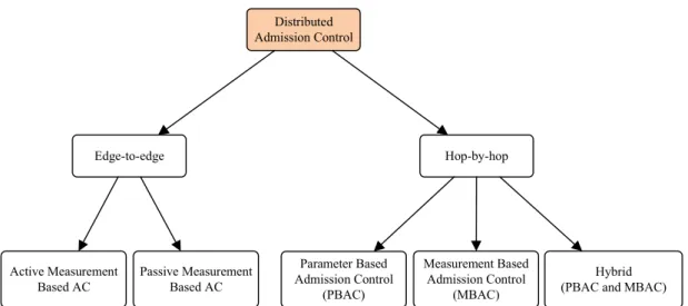
2.2.1 Distributed Admission Control . . . 28

2.2.2 On the Implementation of Admission Control . . . 31

2.2.3 Discussion . . . 32

2.3 WSN Operation and Constraints . . . 33

2.3.1 Hardware and Operating Systems . . . 33

2.3.2 IEEE 802.15.4 Standard - Physical and MAC Layers . . . 34

2.3.3 IP-based stacks . . . 37 ix

x CONTENTS 2.3.4 RPL Routing Protocol . . . 41 2.3.5 Simulation . . . 47 2.3.6 Discussion . . . 48 2.4 Summary . . . 49 3 EED Estimation 51 3.1 EED Estimation Mechanism . . . 52

3.1.1 Internal Delays . . . 53

3.1.2 External Delays and RPL Operation . . . 57

3.1.3 End-to-end Delay Estimation Mechanism Output . . . 57

3.1.4 Validation Environment . . . 58

3.1.5 Results . . . 60

3.2 RPL Modifications . . . 65

3.2.1 Selection of Best Parent Procedure Modifications . . . 67

3.2.2 Update Metrics Procedure Modifications . . . 69

3.2.3 Validation Environment . . . 70

3.2.4 Results . . . 71

3.3 Delay Accounting Optimization . . . 74

3.3.1 Preliminary Experiments . . . 75

3.3.2 Delay Accounting Optimization Procedure . . . 76

3.3.3 Validation Environment . . . 77

3.3.4 Results . . . 77

3.4 Summary . . . 78

4 Distributed Admission Control 81 4.1 Cross-Layer Admission Control Mechanism . . . 81

4.2 Validation Environment . . . 88 4.3 Results . . . 91 4.4 Summary . . . 99 5 Conclusion 103 5.1 Work Review . . . 103 5.2 Contributions Summary . . . 104 5.3 Future Work . . . 105 References 107

List of Figures

1.1 WSN with random and grid topologies . . . 2

1.2 Photo Voltaic Power Plant . . . 3

1.3 WSN topology . . . 4

2.1 IP Stack . . . 10

2.2 Typical communication between a source and a destination node . . . 11

2.3 Delays within nodes in IP networks . . . 13

2.4 Reference points and delay measurement in IP networks . . . 14

2.5 Taxonomy of delay measurement in IP networks . . . 15

2.6 Obtaining PHD without synchronization timer . . . 16

2.7 IETF standards initiatives regarding performance metrics measurement in the Internet . . . 19

2.8 Transporting delays to the estimation points . . . 23

2.9 Network topology providing flow Admission Control . . . 27

2.10 Admission Control mechanisms overview . . . 29

2.11 Time Utility Function for an application requiring soft QoS guarantees . . . 32

2.12 Frames structures defined in the IEEE 802.15.4 standard . . . 36

2.13 TCP/IP and lwIP stacks . . . 38

2.14 uIP and uIPv6 stacks . . . 38

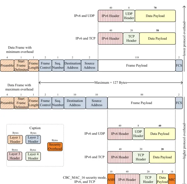
2.15 Protocol overheads in IEEE 802.15.4 standard . . . 40

2.16 Best parent decision using MRHOF in RPL . . . 41

2.17 DIS message format . . . 42

2.18 DIO message format . . . 43

2.19 DAO message format . . . 43

2.20 DAO-ACK message format . . . 44

2.21 RPL control messages and data flow dynamics . . . 45

2.22 DAG Configuration option . . . 46

2.23 DAG Metric Container option . . . 47 xi

xii LIST OF FIGURES

3.1 WSN nodes and End-to-End Delay estimation scope . . . 52

3.2 EEDEM overview . . . 53

3.3 Labels (EEDEM) . . . 54

3.4 Labels and timers (EEDEM) . . . 55

3.5 Average EEDError(MAE)(EEDEM) . . . 61

3.6 Average EEDError(MAPE)(EEDEM) . . . 61

3.7 Average ProcD and PathD distribution (EEDEM) (IGIs from 1 to 10 s) . . . 62

3.8 Average ProcD and PathD distribution (EEDEM) (IGIs from 0.5 to 5 s) . . . . 63

3.9 Average number of RPL packets per node (EEDEM) . . . 64

3.10 Average End-to-End Delay (EEDEM) . . . 64

3.11 Average Packet Reception Ratio (EEDEM) . . . 65

3.12 Selection of best parent procedure (RA-EEDEM) . . . 68

3.13 Hysteresis function graph (RA-EEDEM) . . . 69

3.14 Average EEDError(MAPE)(RA-EEDEM) . . . 72

3.15 Average number of RPL packets per node (RA-EEDEM) . . . 72

3.16 Average End-to-End Delay (RA-EEDEM) . . . 73

3.17 Average Packet Reception Ratio (RA-EEDEM) . . . 74

3.18 Average EEDError(SMAPE)using β varying from 10% to 90% . . . 76

3.19 DAOP integration in EEDEM . . . 77

3.20 MAC queue usage (DAOP) (left: IGI=1 right: IGI=5) . . . 78

3.21 Average EEDError(SMAPE)using different β values and using DAOP . . . 79

4.1 Usefulness Preview function (CLAC) . . . 83

4.2 CLAC mechanism integration . . . 83

4.3 CLAC internal overview . . . 84

4.4 Data packet payload mapped into the internal packet struct (CLAC) . . . 85

4.5 CLAC interaction with the application layer (using AppAPI) . . . 86

4.6 CLAC interaction with the network layer (using NetAPI) . . . 87

4.7 Average EEDError(MAPE)(CLAC) . . . 92

4.8 Average End-to-End Delay (CLAC) . . . 93

4.9 Average Packet Reception Ratio (CLAC) . . . 94

4.10 Average In-profile Packet Ratio and Average Out-of-profile Packet Ratio (CLAC) 96 4.11 Average Packet Usefulness Ratio (CLAC) . . . 97

4.12 Total Energy consumed (CLAC) . . . 98

4.13 Energy consumed mapped in each node (CLAC) . . . 100

List of Tables

2.1 IP-based stacks comparison . . . 39

2.2 Options in RPL Control Messages DIO, DIS and DAO . . . 45

2.3 Routing Metric/Constraint Types and Scopes . . . 47

3.1 Relation between Labels, Functions and Contiki OS Files . . . 54

3.2 EEDEM routing metrics mapped to ROLL metric types . . . 57

3.3 Simulation Parameters (EEDEM) . . . 58

3.4 RA-EEDEM routing metrics mapped to ROLL metric types . . . 67

3.5 Simulation Parameters (RA-EEDEM) . . . 70

3.6 Simulation Parameters (DAOP) . . . 75

4.1 Simulation Parameters . . . 89

4.2 Defined Power Constants . . . 90

List of Abbreviations

#Nodes Number of Nodes [90, 91]

#RcvdPkts Number of Received Packets [59, 60, 71, 75, 82, 88, 89]

#SentPkts Number of Sent Packets [59, 60, 89]

#UsefulPkts Number of Useful Packets [82]

6LowPAN IPv6 over Low Power Wireless Personal Network [39–41]

AC Admission Control [xi, 9, 26–32, 49, 81, 82, 103, 105]

ACK Acknowledge [xi, 16, 17, 42–45, 55, 106]

ACManager Admission Control Manager [84–88]

API Application Programming Interface [84, 85]

APP Application [10, 54, 55]

AppAPI Application API [84–86, 88]

AppID Application ID [85]

ARP Address Resolution Protocol [37]

ARQ Automatic Repeat-reQuest [16, 106]

AS Autonomous System [14, 26–29]

ASH Auxiliary Security Header [39]

BPSK Binary Phase-Shift Keying [35]

CAIDA Center for Applied Internet Data Analysis [20]

xvi List of Abbreviations

CBR Constant Bit Rate [20, 58, 88]

CCA Clear Channel Assessment [36]

CDMA Code Division Multiple Access [20]

CLAC Cross-layer Admission Control [xii, 81–101, 104–106]

CP Candidate Parent [41, 44, 66, 67]

CSMA Carrier Sense Multiple Access [66]

CSMA/CA Carrier Sense Multiple Access / Collision Avoidance [36]

DAG Directed Acyclic Graph [xi, 41–47, 57, 58, 66, 67, 69, 70]

DAO Destination Advertisement Object [xi, xiii, 42–45, 66]

DAOP Dynamic Accounting Optimization Procedure [xii, xiii, 75–80, 104]

DHCP Dynamic Host Control Protocol [37]

Diffserv Differentiated Services [26, 30]

DIO DAG Information Object [xi, xiii, 42–46, 66, 67, 69, 70, 73, 88]

DIS DAG Information Solicitation [xi, xiii, 42, 44, 45, 66]

DNS Domain Name Service [37]

DODAG Destination-Oriented Directed Acyclic Graph [41]

DSSS Direct-Sequence Spread Spectrum [35]

DstID Destination ID [85]

DTSN Destination Advertisement Trigger Sequence Number [42]

EED End-to-End Delay [xii, 2, 4, 5, 7, 9, 11, 15, 18, 28, 31, 34, 51–53, 57–60, 62–66, 70,

71, 73–85, 88–91, 93, 99, 103–105]

EED_RE EED Rough Estimation [67–69]

EEDEM EED Estimation Mechanism [xii, xiii, 52–55, 57–67, 70, 71, 73, 74, 76–81, 88, 99,

List of Abbreviations xvii

EEDError EED Estimation Error [xii, 59–61, 71, 72, 75–79, 88, 91, 92]

EstEED Estimated EED [85, 86, 88]

EstIF EED Estimation Interface [84–86, 88]

ETT Expected Transmission Time [23, 24, 59, 60, 62, 63, 65, 71, 73, 74, 78, 79]

ETX Expected Transmission Count [23, 47, 59, 63]

EWMA Exponential Weighted Moving Average [20–22, 26, 55, 74, 79]

FFD Full Function Device [35]

FIFO First-In-First-Out [32]

FwdD Forward Delay [55, 56]

FwdLinkD Forward Link Delay [56, 57]

FwdProcD Forward Processing Delay [56, 57]

GenD Generation Delay [55, 56, 86]

GenLinkD Generation Link Delay [56, 58]

GenProcD Generation Processing Delay [56, 58]

GPS Global Positioning System [15–17, 20, 25]

GTS Guaranteed Time Slot [36]

HC Header Compression [40]

HopMetric Hop Count Metric [67–70]

HystV Hysteresis Value [67, 69]

IANA Internet Assigned Numbers Authority [46, 47]

ICMP Internet Control Message Protocol [37, 40]

ID Identifier [35, 42, 43]

IEEE Institute of Electrical and Electronics Engineers [xi, 12, 18, 24, 30–37, 39, 40, 48,

xviii List of Abbreviations

IETF Internet Engineering Task Force [xi, 19, 39, 41]

IGI Inter-packet Generation Interval [xii, 59, 60, 62, 63, 65, 70, 71, 73–75, 77, 78, 88, 91,

95, 99]

IGMP Internet Group Management Protocol [37]

Intserv Integrated Services [26]

IoT Internet of Things [1, 34, 37, 106]

IP Internet Protocol [xi, xiii, 1, 9–15, 18, 20, 25, 26, 32, 34, 37–43, 48, 49, 103]

IPPM IP Performance Metrics [19, 20]

IPR In-profile Packet Ratio [xii, 89, 90, 95, 96]

LLN Low-power and Lossy Network [41, 49]

LR-WPAN Low-rate Wireless Personal Area Network [34]

lwIP lightweight IP [xi, 37–39, 48]

MA Moving Average [20–22, 26]

MAC Media Access Control [xii, 11, 12, 24, 35, 39, 54, 55, 58, 68, 70, 76–79, 104]

MAE Mean Absolute Error [xii, 24, 59–61]

MAPE Mean Absolute Percentage Error [xii, 24, 25, 59–61, 71, 72, 88, 91, 92]

MaxEED Maximum EED [81, 82, 85, 86, 88, 91, 95, 99]

MBAC Measurement Based Admission Control [30, 31]

MCU MicroController Unit [33, 34, 90]

MEMS Micro-ElectroMechanical Systems [1]

MIC Message Integrity Code [39]

MinHystV Minimum Hysteresis Value [69]

MIPS Million Instructions Per Second [33]

List of Abbreviations xix

MP2P MultiPoint-to-Point [44]

MRHOF Minimum Rank with Hysteresis Objective Function [xi, 41]

MSE Mean Square Error [24]

MTU Maximum Transmission Unit [39]

NDP Neighbor Discovery Protocol [37]

NetAPI Network API [84, 85, 87, 88]

NTP Network Time Protocol [15–17, 25]

OCP Objective Code Point [46]

OF Objective Function [41, 46, 66, 79]

OF0 Objective Function Zero [41]

OPR Out-of-profile Packet Ratio [xii, 89, 90, 95, 96]

OS Operating System [xiii, 33, 34, 41, 47–49, 54, 88]

OSI Open Systems Interconnection [10]

OWAMP One-Way Active Measurement Protocol [20]

OWD One-Way Delay [14, 15, 17–20, 22, 23, 25, 26]

OWPP One-Way Probe Packet [16, 17]

P2MP Point-to-Multipoint [44]

P2P Point-to-Point [44]

PAN Personal Area Network [34, 35, 37]

PathD Path Delay [xii, 57–59, 62, 63]

PathDMetric Path Delay Metric [57, 58, 63, 66, 67, 70]

PBAC Parameter Based Admission Control [30, 31]

xx List of Abbreviations

PDU Protocol Data Unit [10, 39]

PHD Per-Hop Delay [xi, 14–18, 23, 25, 26]

PHY Physical [10, 11, 39, 49, 54, 58, 70]

PP Preferred Parent [41, 44, 66, 67, 69, 70]

pp percentage points [65, 71, 74, 95]

PPFC Packet Pair Flow Control [17, 23]

PPP Point-to-Point Protocol [37]

ProcD Processing Delay [xii, 11, 12, 25, 34, 57–59, 62, 63]

ProcDMetric Processing Delay Metric [57, 58, 63, 66, 67, 70]

PropD Propagation Delay [12, 16, 17, 25]

PRR Packet Reception Ratio [xii, 60, 65, 66, 71, 74, 78, 79, 82, 89–91, 94, 103, 104]

PSTN Public Switched Telephone Networks [26]

PUR Packet Usefulness Ratio [xii, 82, 89, 90, 95, 97]

QoS Quality of Service [xi, 2, 20, 26–32]

QPSK Quadrature Phase-Shift Keying [35]

QueueD Queue Delay [12, 25, 54–56, 88]

RA-EEDEM RPL Adaptation for EEDEM [xii, xiii, 65–74, 79, 80, 104]

RAM Random-Access Memory [33, 34, 37, 39, 48]

RcvD Receiver Delay [55, 56]

RcvLinkD Receiver Link Delay [56, 57]

RcvProcD Receiver Processing Delay [56, 57]

RFC Requests For Comments [19, 20, 39–42, 46, 47]

RFD Reduced Function Device [35]

List of Abbreviations xxi

RMSE Root Mean Square Error [24]

ROLL Routing Over Low-power and Lossy networks [xiii, 41, 47, 57, 67]

ROM Read-Only Memory [33, 34, 37, 39, 48]

RPL IPv6 Routing Protocol for Low-Power and Lossy Networks [xi–xiii, 5, 26, 34, 41–47,

49, 52, 57–59, 63–67, 70–72, 74, 78, 79, 83–85, 88, 104–106]

RPLIF RPL Interface [84, 85, 88]

RTD Round Trip Delay [14, 19]

RTT Round Trip Time [14, 18, 23]

SELF-PVP SELF-organizing power management for Photo-Voltaic Power plants [2]

SeqNr Sequence Number [85]

SICS Swedish Institute of Computer Science [34]

SMAPE Symmetric MAPE [xii, 24, 25, 75–79, 88]

SNMP Simple Network Management Protocol [37]

SrcID Source ID [85]

TCP Transmission Control Protocol [xi, 10, 32, 37, 38]

TotalDMetric Total Delay Metric [67, 69]

TransD Transmission Delay [12, 16, 17, 25, 34, 54–56, 88]

TUF Time Utility Function [xi, 31, 32]

TWAMP Two-Way Active Measurement Protocol [20]

TWD Two-Way Delay [14, 15, 17–19, 25]

TWPP Two-Way Probe Packet [17]

UDGM Unit Disk Graph Medium [58, 88]

UDP User Datagram Protocol [37, 40, 58, 70, 75, 88]

UP Usefulness Preview [xii, 82, 83]

WG Working Group [19]

WLAN Wireless Local Area Network [16]

WMA Weighted Moving Average [20–22, 26]

WMN Wireless Mesh Network [12, 18, 28]

WPAN Wireless Personal Area Network [34, 39]

WSN Wireless Sensor Network [xi, xii, 1–5, 7, 9, 12, 16, 18, 22, 25, 26, 30–34, 41, 47–49,

Chapter 1

Introduction

Recent advances in the scaling of electronic circuits and in providing them with the ability to interact with the world around, enabled the appearance of Micro-ElectroMechanical Systems (MEMS). MEMS technology combines very small computers with sensor and control capabilities. MEMS mass commercialization and distribution made it very cost-effective and suitable for multiple uses. The deployment of communications capabilities in MEMS fostered the appearance of new network architectures and their interconnection to the existing global Internet Protocol (IP) network leaded to the birth of the Internet of Things (IoT) concept. The IoT envisions a world of interaction and coordination between objects, with or without human intervention, for the creation of smart environments.

Wireless Sensor Network (WSN) architectures extend the IoT concept by giving wireless communications capabilities to MEMS. A WSN is composed of a large number of sensor nodes, where each node can be characterized as a very small computer with a wireless interface. These nodes generate data from their sensors, such as temperature, humidity, moisture, and pressure, among others, and forward this data towards a gateway node. The gateway node, in turn, connects these networks to the Internet, as shown in Figure 1.1. WSN applications are multifold in areas such as smart metering, health care, environmental sensing, home automation, sports and wellness.

The hardware of the sensor nodes in a WSN is designed with processing and communica-tions constraints since these nodes have limited energy resources. Even though these hardware limitations exist, more recently new and more complex applications and services (e.g. audio and video streaming) are pushed to be supported by the WSNs, in order to foster the concept of the IoT. These initiatives create new challenges in networking research areas such as routing, management, quality of service and energy efficiency.

2 Introduction Caption Grid Topology WSN Random Topology WSN 2 3 4 5 8 9 11 12 13 15 16 17 1 6 7 10 Internet 3 17 10 Internet 1 13 12 6 5 15 7 2 11 9 8 16 4 14 14 WSN node

Gateway node Wireless Range Data Flow

Figure 1.1: WSN with random and grid topologies

1.1

Scope and Motivation

This thesis was carried out in the scope of the SELF-organizing power management for Photo-Voltaic Power plants (SELF-PVP) project [1] that aimed to increase the efficiency of a photo voltaic power plant with approximately 200.000 solar panels distributed in an area of 250 hectares. The solar panels include sensor nodes that communicate with each other using a grid topology WSN as shown in Fig. 1.2. In this scenario, we aim to deploy real-time applications, such as monitoring or video surveillance, in a set of sensor nodes.

Real-time applications typically generate traffic flows with Quality of Service (QoS) re-quirements that can be defined in terms of delay, jitter or packet loss. In case these applications require strict delay boundaries from source to destination, their packets must be delivered to the destination application within an End-to-End Delay (EED) limit in order for the information to be considered useful. The packets delivered outside the defined EED limit will be considered useless and discarded by these applications at the destination.

1.2 Problem Statement 3

Photo Voltaic Power Plant

Caption

Sensor node

Wireless communications range Solar panel

...

...

...

...

...

...

...

...

...

...

Figure 1.2: Photo Voltaic Power Plant

processing and communications constraints, we explore the idea that the WSN should avoid processing and transporting useless packets and use its full potential to maximize the number of delivered useful packets. Therefore, our research is oriented towards the enhancement of the performance of a grid WSN considering the application’s viewpoint, while taking into consideration the efficient use of the available resources.

1.2

Problem Statement

A real-time application is to be deployed on a grid WSN where each node has limited resources in terms of processing, communications and energy. The real-time application generates delay sensitive flows with data that is assumed to be useful for the destination only if it is received within a strict delay boundary, and useless otherwise. In order to enhance the support for this application, the WSN performance can be oriented to maximize the number of delivered useful packets. At the same time, since WSN nodes have relevant processing, transmission and energy constraints, they should avoid to process and transport the useless packets.

The main problem to address is that the usefulness of a packet is determined at its destination, and processing, transmission and energy resources have already been expended

4 Introduction to transport the packet. Since the destination application may not consider all received packets as useful, if we are able to identify, as soon as possible, which packets will likely miss the application delay deadlines and avoid their transmission to the network, an increase in network performance and energy efficiency is expected to be achieved.

1.3

Objective

The main objective of this thesis is to enhance the support of real-time applications in a grid WSN topology, as shown in Fig. 1.3. In this topology, each source node generates a delay sensitive data flow directed towards a central destination node.

WSN

Wireless communications range

Figure 1.3: WSN topology

In each source node, the chosen strategy is to preview the EED of each packet and, as earlier as possible, avoid packet transmissions when these are expected to not comply with the limits given by the application. In order to pursue this strategy, the research efforts are divided in two particular objectives:

• Provide an EED estimation mechanism to be deployed in a WSN with minimal impact

on network performance;

• _{Provide a WSN admission control mechanism based on the EED estimation and intended}

1.4 Contributions 5

1.4

Contributions

This thesis provides two main original contributions:

• Novel mechanism to estimate EED based on RPL routing protocol

∗ In order to preview if a packet will be delivered within the EED limit defined

by the application, a novel EED estimation mechanism is proposed. Other delay estimation mechanisms are proposed in literature but some of them do not provide a real-time and per-packet delay estimation, while others introduce additional traffic in the WSN to provide estimations. The proposed EED estimation mechanism provides a real-time and per packet EED estimation using IPv6 Routing Protocol for Low-Power and Lossy Networks (RPL). RPL packets are used to feedback the EED delay of the previously sent packets to the source nodes, thus avoiding extra traffic in the WSN. Also, to enhance EED estimation accuracy, this proposal accounts not only with transmission delays but also with the in-node processing delays which are relevant in the context of the limited processing resources of the nodes. This contribution has been published in [2]. Also, a set of RPL modifications to enhance the accuracy of EED estimation were proposed, and published in [3]. In the context of the EED estimation mechanism and in order to enhance EED estimation when using multiple network loads, a delay accounting optimization procedure was also proposed, and published in [4].

• Novel cross-layer admission control mechanism based on the EED estimation

∗ In order to decide if a packet should be transmitted accordingly to their usefulness

to the destination application, a novel cross-layer packet admission control mech-anism is proposed. The proposed admission control mechmech-anism is distributed by the WSN nodes and it is responsible for the decisions to transmit or drop a packet according to the requirements defined by the application. Other admission control mechanisms are proposed in the literature but the novelty of the proposed mecha-nism is that it runs in a cross-layer operation mode involving the application and network layers, while implementing interfaces with the EED estimation mechanism and RPL routing protocol. This contribution has been accepted for publishing in [5].

6 Introduction

1.5

Publications

• Pedro Pinto, António Pinto, and Manuel Ricardo, “Data and Path Aggregation in

Large Scale and Cluster-based Wireless Sensor Networks”, in MAPTele Workshop, Aveiro, Portugal, May 2011.

• Pedro Pinto, António Pinto, and Manuel Ricardo, “Secure Data and Path Aggregation

in WSN (Poster)”, in MAPTele Workshop, Porto, Portugal, Jun. 2012.

• Pedro Pinto, António Pinto, and Manuel Ricardo, “End-to-end Delay Estimation

using RPL Metrics in WSN”, in Proceedings of the Wireless Days (WD’2013), IFIP, Valência, Spain, Nov. 13-15, 2013, pp. 1–6.

• Pedro Pinto, António Pinto, and Manuel Ricardo, “RPL Modifications to Improve

the End-to-end Delay Estimation in WSN”, in Proceedings of the 11th International Symposium on Wireless Communications Systems (ISWCS), IEEE, Barcelona, Spain, Aug. 2014, pp. 868–872.

• Pedro Pinto, António Pinto, and Manuel Ricardo, “Reducing WSN Simulation

Run-time by using Multiple Simultaneous Instances”, in Symposium on Modelling and

Simulation in Computer Sciences and Engineering (ICNAAM 2014), Rhodes, Greece, Sep. 2014.

• _{Pedro Pinto, António Pinto, and Manuel Ricardo, “Delay Accounting Optimization}

Procedure to Enhance End-to-End Delay Estimation in WSNs”, in Proceedings of the 8th International Wireless Internet Conference (WICON 2014) - Symposium on Wireless and Vehicular Communication, Lisbon, 2014.

• Pedro Pinto, António Pinto, and Manuel Ricardo, “Reducing Simulation Runtime in

Wireless Sensor Networks: A Simulation Framework to Reduce WSN Simulation

Runtime by Using Multiple Simultaneous Instances (Book Chapter),”in Handbook

of Research on Computational Simulation and Modeling in Engineering, IGI Global, 2016. 726-741. 8 Sep. 2015. ISBN: 978-1-4666-8823-0.

• Pedro Pinto, António Pinto, Manuel Ricardo, “Delay Accounting Optimization

Proce-dure to Enhance End-to-End Delay Estimation in WSNs”(Book Chapter), Wireless

Internet Book - Lecture Notes of the Institute for Computer Sciences, Social Informatics and Telecommunications Engineering. Revised Selected Papers of the 8th International

1.6 Document Structure 7

Conference, WICON 2014, Lisbon, Portugal, Nov. 13-14, 2014. Volume 146. May 21th, 2015. ISBN: 978-3-319-18801-0.

• Pedro Pinto, António Pinto, and Manuel Ricardo, “Cross-layer Admission Control

Mechanism to Enhance the Support of Real-time Applications”, Sensors Journal, IEEE, vol. 15, no. 12, pp. 6945–6953, Dec. 2015.

1.6

Document Structure

The structure of this thesis is as follows. Chapter 2 reviews the related work regarding the EED estimation and admission control research areas. It also describes specific operations and constraints present in the WSNs. Chapter 3 details and evaluates the EED estimation mechanism, and the implemented improvements that enhance the EED estimation. Chapter 4 details and evaluates the proposed packet admission control mechanism. Finally, Chapter 5 concludes the thesis and discusses future work.

Chapter 2

Delay Estimation and Admission

Control in IP Networks

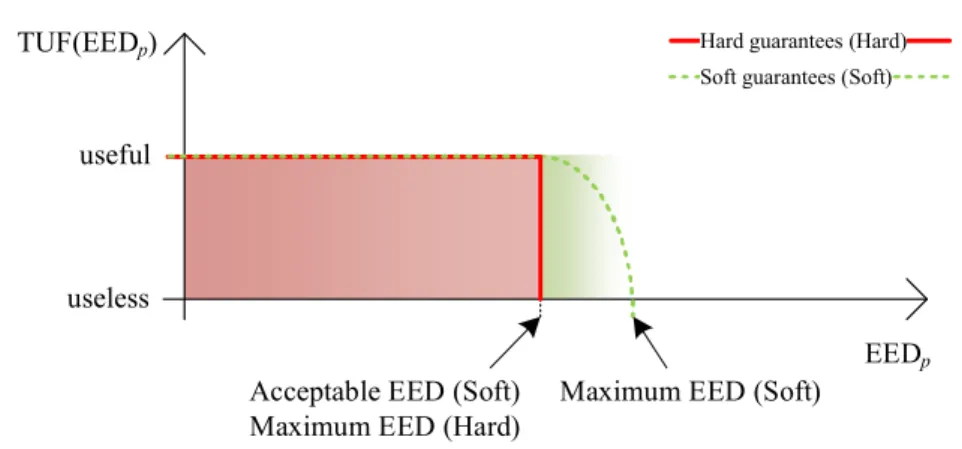
Real-time applications require specific EED boundaries (between source and destinations nodes) for all its packets. At the destination, if packets are delivered within the defined EED boundary they are considered useful; by contrary, if the packets are delivered outside this time boundary they will be considered useless and will be discarded at destination.

In order to preview the usefulness of a packet, the delay from source to destination must be estimated in each node. Section 2.1 presents the state of the art on delay measurement and esti-mation. In order to actively control the admission of new traffic and avoid transmitting packets that potentially will miss the defined EED limit, an Admission Control (AC) mechanism is necessary. Section 2.2 presents the state of the art on AC in IP networks.

Since the envisioned application must be supported by a WSN, the particular operation procedures and relevant constraints of these networks are also described in Section 2.3. This Chapter is summarized in Section 2.4.

2.1

Delay Estimation in IP Networks

The expansion of the packet-switched networks in early 90s facilitated the interconnection of different network architectures. However these networks provide little control over the packet delay at the forwarding nodes [6]. Since then, several research efforts were made in order to characterize, measure and estimate packet delays in the Internet, or global IP network.

10 Delay Estimation and Admission Control in IP Networks

2.1.1 Delays Definition

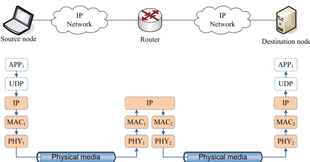
To be a part of an IP network, a node must implement an IP network stack. Fig. 2.1 presents the Open Systems Interconnection (OSI) and TCP/IP models, and a TCP/IP stack with a common combination of protocols which use IP as the center protocol. These protocols perform functions specified in the depicted models from Physical (PHY) layer to Application (APP) layer implemented in hardware, or software, or both. The TCP/IP model is used as reference in this thesis.

Layer 7 Layer 6 Layer 5 Layer 4 Layer 3 Layer 2 Layer 1 TCP/IP model OSI model Application Presentation Session Transport Network Data Link (MAC) Physical (PHY)

Transport Application (APP)

Network Data Link (MAC) Physical (PHY) TCP/IP stack UDP APP1 IP MAC1 PHY1 TCP APPn APP2 MACn PHYn MAC2 PHY2 ... ... … Figure 2.1: IP Stack

When an application sends data, it uses the set of protocols of the stack to transmit it from

the source to the destination nodes according to Fig. 2.2. In this case the application APP1

passes data to lower layers which in turn send it to the PHY layer. The router de-encapsulates the received information up to IP protocol an forwards it through another interface. The information eventually reaches the destination node. Since this information is successively encapsulated and de-encapsulated, different types of Protocol Data Unit (PDU) are formed (e.g. segments, datagrams, packets, or frames). For simplicity, these different PDUs are referred as packets for the rest of this thesis.

2.1 Delay Estimation in IP Networks 11 UDP APP1 IP MAC1 PHY1 UDP APP1 IP MAC2 PHY2 IP MAC1 PHY1 MAC2 PHY2 IP Network Router IP Network Destination node Source node

Physical media Physical media

Figure 2.2: Typical communication between a source and a destination node

By definition, a delay is a time interval which is obtained by the difference of two time instants tAand tB, where tA< tB, as follows:

Delay = ∆t = tB− tA (2.1)

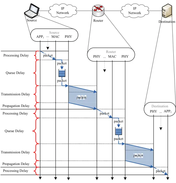
In the IP networks, the time instants are collected at reference points. When a packet progresses from source to destination, different delay components can be accounted in each node. Fig. 2.3 presents a source node sending a packet to a destination node where the following four delay components can be depicted:

• Processing Delay (ProcD): is the time required to process a packet within a node.

This delay includes not only the time elapsed while performing layer 3 and above layers tasks, but also the tasks within PHY and Media Access Control (MAC) layers when packet is received. In the IP networks this delay depends on the number of tasks and on the computational power available. In [7] the authors present an analysis of EED measurements in IP networks performed by Réseaux IP Européens Network Coordination Centre (RIPE NCC) by using probe packets where it is assumed that the ProcD is dependent of three factors: the protocol stack, the the computational power available at each node and the link driver. Also, the authors verified that the processing delays are not the same for different probe-packets due to the variability of tasks performed in the router and they split the processing delay in two parts: the stochastic and

12 Delay Estimation and Admission Control in IP Networks the deterministic. The processing delay component is often neglected by many research efforts when accounting delays in a IP network; however, this delay component may be significant on scenarios characterized by wireless devices with limited processing resources, such as those used in WSNs. As example, in [8] the authors present a delay analysis for a Wireless Mesh Network (WMN) using IEEE 802.11 devices in which each mesh node accounts with intra-node processing delays. In [9] and in [10] the authors account the ProcD to provide accuracy to their delay estimation.

• Queue Delay (QueueD): is the time elapsed since the packet enters the MAC queue,

waiting for transmission, until it leaves this queue to be transmitted. This delay is essentially dependent of the network load. Queue theory [11] can provide an estimation for this delay component.

• Transmission Delay (TransD): is the time required to push all the packet into the physical

media. This delay is proportional to the packet’s length and can be obtained using:

TransD (s) = length of packet (bit)

rate of transmission (b/s) (2.2)

• Propagation Delay (PropD): is the amount of time required to move a bit of the packet

from one node to the next node. This delay is proportional to the distance between the nodes and can be obtained using:

PropD (s) = distance between nodes (m)

signal propagation speed (m/s) (2.3)

The signal propagation speed is dependent of the physical media used. For instance, in wireless networks the propagation speed is approximately the speed of light, denoted by

the constant c, which is approximately 3.00 × 108 _{m/s; when using a copper wire the}

signal propagation is around 2/3 of c, i.e. approximately 2.00 × 108_{m/s. For a distance}

of 10 m between nodes and using wireless medium, the PropD assume values around 33.3 ns and thus, in some scenarios, the PropD is neglected.

Using the delay definitions above, the total delay in a node can be obtained using the following equation:

2.1 Delay Estimation in IP Networks 13 Router Processing Delay IP Network Router IP Network ... Destination ... APP1 Destination Source MAC packet Queue Delay Transmission Delay Source ... MAC APP1 PHY Propagation Delay packet packet Queue Delay Processing Delay Propagation Delay packet PHY packet packet packet packet PHY PHY Processing Delay packet Transmission Delay

Figure 2.3: Delays within nodes in IP networks

2.1.2 Delays Measurement

In order to measure packet delays in IP networks two reference points are required. Timestamps must be collected when packets pass through these reference points and delays are accounted in a unique location by using these timestamps. Different scales can be used for these reference points; in a node scale these reference points may refer to code execution points; in a macro scale these reference points may refer to two routers located in distant geographical positions.

14 Delay Estimation and Admission Control in IP Networks Measuring delays using Layer 3 reference points

Fig. 2.4 presents a set of layer 3 reference points and, using them, three types of delays can be defined: Per-Hop Delay (PHD), One-Way Delay (OWD), Two-Way Delay (TWD), also named Round Trip Delay (RTD) or Round Trip Time (RTT). The same definition is used in [12]. Caption Reference Points IP Network Router Router IP Network Source _Destination IP Network PHD TWD PHD PHD

Source Router Destination Initial Reference Point Final Reference Point

Initial Reference Point &

Final Reference Point

OWD

path of packet flow

Final Reference Point Initial Reference Point

Figure 2.4: Reference points and delay measurement in IP networks

PHD accounts the delay experienced by a packet between two network reference points distant one hop from each other, named initial reference point and final reference point. The OWD is the delay of a one way packet between initial and final reference points involving multiple intermediate hops and IP networks, e.g. a source and a remote destination node or two edges of an Autonomous System (AS). In case the reference points are the packet source and

2.1 Delay Estimation in IP Networks 15

destination, the OWD can be assumed as the packet EED. The TWD is the round trip delay of a packet, i.e, both initial and final reference points are in the same node or reference point.

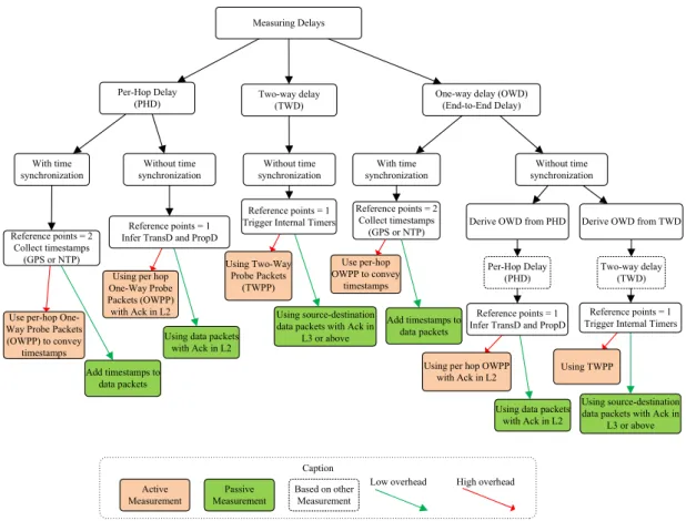
Fig. 2.5 proposes a taxonomy regarding methods for measuring these delays. For each method it is indicated if the measurement is active or passive, i.e. if the measurement procedure generates additional traffic or not. Also, for each method it is indicated if a high or a low overhead is introduced when measuring the delay.

Measuring Delays

Two-way delay (TWD)

One-way delay (OWD) (End-to-End Delay) Reference points = 2 Collect timestamps (GPS or NTP) With time synchronization

Derive OWD from TWD Without time

synchronization Per-Hop Delay

(PHD)

Using per hop One-Way Probe Packets (OWPP) with Ack in L2

Derive OWD from PHD

Using data packets with Ack in L2 Without time synchronization Two-way delay (TWD) Per-Hop Delay (PHD) Reference points = 1

Infer TransD and PropD

Without time synchronization Using Two-Way Probe Packets (TWPP) Using source-destination data packets with Ack in

L3 or above Reference points = 2 Collect timestamps (GPS or NTP) With time synchronization

Using data packets with Ack in L2 Reference points = 1 Infer TransD and PropD

Using TWPP Caption Passive Measurement Active Measurement

Low overhead High overhead Use per-hop

One-Way Probe Packets (OWPP) to convey

timestamps

Add timestamps to data packets

Reference points = 1 Trigger Internal Timers

Reference points = 1 Trigger Internal Timers Use per-hop

OWPP to convey timestamps

Add timestamps to data packets

Using per hop OWPP with Ack in L2

Using source-destination data packets with Ack in

L3 or above

Based on other Measurement

Figure 2.5: Taxonomy of delay measurement in IP networks

To measure PHD, when Global Positioning System (GPS) or Network Time Protocol (NTP) is available, nodes can be synchronized so that the hardware clocks of source and destination have the same reference time. In the case of using NTP, specific probe packets are used to transport the timestamps. The NTP is widely used in the Internet for clock synchronization and it provides an accuracy to the order of milliseconds over time scales of hours to days; however systematic errors can be verified as show in [13]. If GPS is used, the timestamps can be inserted directly in the data packets which enables to minimize the measurement overhead. Therefore, in this measurement method, a timestamp is collected in the initial reference point,

16 Delay Estimation and Admission Control in IP Networks this timestamp is transmitted to the next hop node, and since the next node is the final reference point, it collects another timestamp, and calculates the difference between the two collected timestamps to obtain the PHD. Two options are available to transport the first timestamp to the next node: to use a per hop One-Way Probe Packet (OWPP) that includes the timestamp, or add the timestamp to a data packet. The former uses a specific packet and the latter uses normal data packets which in general introduce less overhead in the measurement procedure.

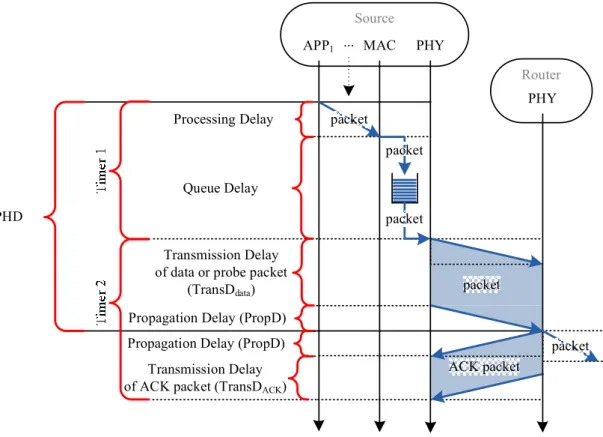
GPS or NTP may not be available or may not work under some situations as indoor areas. In this case, the nodes are not synchronized and the PHD must be measured within each node, i.e. with initial and final reference points in the same reference point. This is accomplished by measuring the delays as presented in Eq. 2.4 by using internal timers, except for the TransD and the PropD (see Fig. 2.3) for which the delays must be inferred.

Fig. 2.6 presents a node and its next hop where PHD is to be obtained using per hop OWPP or data packets and using a L2 stop and wait Automatic Repeat-reQuest (ARQ) procedure, which consist in an automatic Acknowledge (ACK) in L2 when the packet is correctly received, which is commonly used in Wireless Local Area Networks (WLANs) and WSNs.

Router

Queue Delay

Transmission Delay of data or probe packet

(TransDdata)

Source

... MAC APP1

Propagation Delay (PropD)

packet packet packet packet Processing Delay ACK packet PHY PHY Transmission Delay of ACK packet (TransDACK)

Propagation Delay (PropD) packet

PHD

2.1 Delay Estimation in IP Networks 17

From the Fig. 2.6, the PHD can be obtained using:

PHD = (Result of Timer 1) + TransDdata+PropD (2.5)

where TransDdatacan be obtained using:

TransDdata=(Result of Timer 2) − (2 × PropD + TransDACK) (2.6)

Thus, PHD can be obtained as:

PHD = (Result of Timer 1) + (Result of Timer 2) − PropD − TransDACK (2.7)

Assuming a specific physical media the PropD can be approximated using the Eq. 2.3, and

the TransDACK can be approximated using the Eq. 2.2. This procedure is possible if ACK

is enabled in L2. An alternative approach to measure the TransD using probe packets in one reference point is named Packet Pair Flow Control (PPFC) and is proposed in [14]. PPFC is intended to be used in steady networks and it is based on the idea that if two probe packets are sent directly after each other, they are also queued one after the other and the time which lies between the end of the reception of the first packet and the start of the reception of the second packet, can be inferred as the transmission time.

When measuring TWD, both initial and final reference points are defined in the same node, i.e. there is a single reference point. Thus, time synchronization is not required and this type of delay is easily measured by triggering internal timers that account for the delay since the packet is sent, until an answer or echo is received. A Two-Way Probe Packet (TWPP), e.g. generated by ping or traceroute utilities, or any source to destination packet with ACK in L3 or above can be used to trigger the timers and collect the TWD.

In order to measure the OWD, the network nodes can be synchronized (using GPS or NTP) or not. If the nodes are synchronized, the timestamps are collected at two different reference points and OWD is measured. To transport the timestamp from one reference point to the other, OWPPs can be used or the timestamps can be added to normal data packets. If nodes are not

synchronized, two options are available: to derive OWD from PHD1_{or to derive OWD from}

1_{Network delay tomography operates in reverse, i.e. measures OWD and infers PHD. Further reading regarding}

18 Delay Estimation and Admission Control in IP Networks TWD. If OWD is derived from PHD, Eq. 2.8 or Eq. 2.9 can be used.

OWD = PHD × N (2.8)

OWD =

_∑

i=1

PHDi (2.9)

where PHDi is the PHD obtained in node i and N is the number of nodes up to the

final reference point. The accuracy provided by the Eq. 2.8 to derive OWD from PHD is highly questionable since, in the real scenarios, individual PHDs may be different and even uncorrelated. Eq. 2.9 should provide more accurate results but individual PHD must be obtained in all the nodes transversed by packets.

Authors in [20] present a proposal to estimate OWDs in IP networks by conducting measurements of transmission, propagation and queuing delays in each node. In the context of wireless networks, in [21] the authors provide an analysis on the minimum delay in a WSN using unslotted mode of IEEE 802.15.4, taking into account the transmission related times, such as back off periods and inter-frame spacing. In [22] the authors propose an EED-based routing protocol for a WMN intended to to minimize EED accounting with queuing and transmission delays. In [9] the authors present a cross-layer mechanism to guarantee a defined EED for time sensitive applications that uses the IP-header option field to accumulate the PHD estimate that is used by a forwarder node to select an output priority queue.

In the case of the OWD being derived from TWD, Eq. 2.10 can be used.

OWD =TWD

2 (2.10)

In [23] authors provide a procedure to estimate TWD in multicast scenarios by using probe packets. Authors in [24] present a model focused on the prediction of the TWD obtained using statistical functions over previous measurements of TWD. In [25] the authors observed that RTT is a poor approximation of the OWD and proposed a scheme that analytically derives the OWD, forward and reverse delay for asymmetric networks. Also, the analysis made in [26, 27] reveals that the Internet paths have large delay asymmetries, raising doubts about the accuracy of this method when used with real traffic.

2.1 Delay Estimation in IP Networks 19

IETF Efforts to Measure Delay in IP networks

In order to provide common understanding regarding performance and reliability metrics that could be adopted in the Internet, Internet Engineering Task Force (IETF) has defined frameworks and methodologies to measure metrics in the Internet such as delay, bandwidth, throughput and packet loss. Fig. 2.7 presents the major IETF contributions in this area. They come mainly from IP Performance Metrics (IPPM) Working Group (WG).

RFC 2330 May 1998 Set 1999 RFC 7312 Aug 2014 RFC 2681 RFC 2679 RFC 2680 RFC 2678 Nov 2002 RFC 3393 Sep 2006 RFC 4656 RFC3432 Sep 2008 RFC 5357 Framework for IP Performance Metrics (IPPM) A One-Way Delay Metric for IPPM

A Round-trip Delay Metric for IPPM

Network performance measurement with periodic streams A One-Way Active Measurement Protocol (OWAMP)

Advanced Stream and Sampling Framework

for IPPM IPPM Metrics for

Measuring Connectivity

A One-Way Packet Loss Metric for IPPM

IP Packet Delay Variation Metric for IPPM

A Two-Way Active Measurement Protocol (TWAMP) Apr 2010 RFC 5835 Framework for Metric Composition

Figure 2.7: IETF standards initiatives regarding performance metrics measurement in the Internet

In RFC 2330 [28] the IPPM WG defines a general framework and concepts to which performance metrics should comply to, and possible measurement methodologies. These metrics can be derived from other metrics that exhibit spatial, or temporal composition. The methodologies highlighted to measure these metrics fall in three categories: 1) direct measurement by injecting test traffic; 2) project end-to-end metrics from measured hop metrics; 3) estimate a metric from other sets of metrics.

The RFC 2678 [29] defines a set of metrics for connectivity between a pair of Internet nodes over a time interval and the RFC 2680 [30] defines metrics for one-way packet loss across Internet paths. The RFC 2679 [31] defines a metric for OWD and the RFC 2681 [32] defines a metric for TWD of packets in context of IPPM across Internet paths. Both contributions highlight that there are scenarios where OWD measurement should be performed instead of the RTD measurement since the path from a source to a destination can be different than the reverse path and even when two paths are symmetric, they may have different performance characteristics due to asymmetric queuing. Also, the performance of an application may

20 Delay Estimation and Admission Control in IP Networks depend mostly on the performance in one direction and in the use of QoS enabled networks, so provisioning in one direction maybe different than provisioning in the reverse direction, and thus the QoS guarantees differ.

The RFC 3393 [33] defines a metric for characterizing the variation of packets delays across Internet, which is based on the difference between OWD of selected packets. RFC 3432 [34] describes a periodic sampling method and relevant metrics for assessing the performance of IP networks using active and passive measurements and simulating applications generating Constant Bit Rate (CBR) traffic, typically multimedia applications.

RFC 4656 [35] presents the One-Way Active Measurement Protocol (OWAMP) for uni-directional metrics such as OWD and one-way loss using time sources such as GPS and Code Division Multiple Access (CDMA)-based systems (e.g. cellular networks) by using probe packets. The Center for Applied Internet Data Analysis (CAIDA) [36] uses OWAMP to measure one-way latency. Since OWAMP does not accommodate round-trip or two-way measurements, RFC 5357 [37] proposed the Two-Way Active Measurement Protocol (TWAMP) that can be used to measure one-way metrics in both directions between two network elements.

RFC 5835 [38] provides a framework for classes of metrics such as temporal aggregation, spatial aggregation, and spatial composition, that were described in the original IPPM frame-work (RFC 2330). RFC 7312 [39] updates the RFC 2330 with advanced considerations for measurement methodology and testing.

2.1.3 Delays Estimation

Two types of strategies can be used to estimate delays: offline and real-time. The offline strategy, takes advantage of theoretical models such as queuing theory or network calculus. The real-time strategy, estimates delays using samples of packets delays.

In an IP network, the sequence of packet delays measured can be described as a time series. The forecast methods based on time series use past data to estimate future data items and these methods are used in areas such as business planning or weather forecast [40, 41]. Therefore, real-time packet delay forecast or estimation comprehends two steps: 1) collect previous packet delays and 2) based on the previous packet delays provide an estimate for future packet delays. If the time series can be defined as stationary, i.e. no systematic change in key statistical moments such as the mean or variance, the following estimation methods can be used: naive, Moving Average (MA), Weighted Moving Average (WMA) and Exponential Weighted Moving Average (EWMA).

2.1 Delay Estimation in IP Networks 21

Assuming that Dnis the delay of the n-th sample, its estimate defined asDcncan be obtained

using naive method as follows:

c

Dn= Dn−1 (2.11)

Using the MA method, theDcnis obtained as follows:

c Dn= 1 N N−1

∑

where N is the number of previous delays to consider.

Using the WMA method, theDcnis obtained as follows:

c Dn= 1 N N−1

∑

Wi is the weight for the item i, where ∑N−1_i=0 Wi=1

Nis the number of previous delays to consider

Using the EWMA, theDcnis obtained as follows:

c

Dn= β .Dn−1+ (1 − β ).Ddn−1 (2.14)

where β is the smoothing factor and 0 < β < 1

The naive method simply assumes that the next delay will be equal to the last one obtained, ignoring any historical data.

The MA method is often used as it is easy to understand and compute, but the estimation is only available when data series are equal or greater than N. The MA method also tracks the actual data but presents it with a lag and weights the data equally, which means it is not able to adequately represent data outliers (i.e. data points distant from other observations)[42].

In order to cope with some of this issues, WMA method can be used. WMA method counts differently the recent data and the other periods data in order to better adjust to the properties of the time series. Even though the result of WMA method also presents lag when compared to the time series and, similarly to the MA method, it is highly dependent on the value of N.

22 Delay Estimation and Admission Control in IP Networks The EWMA method is easy to compute in real-time. Older data points never leave the estimation results but their impact is reduced for each new item in data series. Another feature regarding the EWMA is that it does not use many memory resources. While MA and WMA methods require the entire data set to be stored in memory, EWMA only needs the last estimation and the last sampled value. Due to these advantages many techniques use EWMA for forecasting. Authors in [43] propose an adaptive scheme based on EWMA to provide fault tolerant sensor networks and balance between traffic overhead and transmission failure, using multipath routing. In [44] authors propose a link quality monitoring mechanism where EWMA is employed to smooth the monitoring results. In [45] and [46] the authors propose prediction algorithms based on a moving average to be used in solar panels, and compare these methods with EWMA. In [47] the authors propose a link quality evaluation algorithm which employ EWMA method to adjust its sensitivity. Authors in [48] propose a prediction model to forecast the expected energy intake in a wireless sensor node, whose performance is compared with EWMA-based solutions. In [49] the authors propose the use of routing metrics accounting with average queuing and transmission delays obtained using EWMA. In [50] the authors use a data aggregation mechanism to reduce redundant packets by taking into account their current data smoothed by a EWMA function.

Although the methods described above can be used to forecast delay values based on the previous experienced delays, the estimate can be requested in a different network node from that in which the estimate was obtained. In this case, after providing a delay estimate, it is necessary to transport it to the nodes where the estimation is required. As example, when measuring OWD the second timestamp is the final reference point (see Fig. 2.4), and thus the delay estimate will be obtained in final node. If the source node is required to have this estimate it is necessary to transport the estimate up to the source node.

The Fig. 2.8 presents three methods that can be used to feedback delay information to where it is needed, here named as the estimation points. The terms active and passive feedback are used similarly to active and passive measurement, i.e. to indicate if the method influences more or less the traffic that is already transported in the network. The methods that use specific messages, e.g. using their own packets, have the undesired effect of introducing additional traffic, which in turn contributes to consume energy and processing resources, which is highly undesirable in WSN scenarios. In order to avoid extra traffic, the delay information can be conveyed in packets that are already transported in the network, i.e. conveyed in data plane messages or in control plane messages. In order to feedback delays using the data plane messages it is necessary that data packets are transported in reverse direction from source

2.1 Delay Estimation in IP Networks 23

to destination node. In case of real-time applications the traffic can be highly asymmetric or not provide any data packets in reverse direction at all. The feedback can also be provided by using control plane messages, more particularly using the routing protocol messages. In [51] the authors survey routing metrics related to delays accounting that can be used in this context.

Transport delays to Estimation Points

Using data plane messages Using control plane messages

Convey info in routing protocol packets Using applications packets Using ETT-based metrics ? Using specific messages

? Using own application packets Caption Passive Transport Active Tranport

High overhead Low overhead To explore ?

Figure 2.8: Transporting delays to the estimation points

The research proposals that use routing protocol messages to feedback previous delays, use Expected Transmission Time (ETT) or ETT-related metrics, which can be derived from metrics such as the Expected Transmission Count (ETX) as shown in [52]. The ETT can be derived from ETX by using Eq. 2.15, where ETX is the expected number of transmission attempts required for successfully transmitting a packet, S is the packet size, and D is the data rate of the link.

ETT = ETX × S

D (2.15)

Authors in [53] provide studies to derive the OWD from the PHD or from the RTT. This work also used a wireless testbed to compare the performance of RTT and PPFC when used as link quality routing metrics against the performance of the ETX and hop count. The results provided showed that only ETX was able to outperform the hop count metric, whereas the

24 Delay Estimation and Admission Control in IP Networks two delay based metrics performed poorly. In [54] the authors propose a ETT-based metric intended to provide routing efficiency under various link conditions. In the proposed metric the MAC layer overheads are taken into account for calculating the data transmission time, instead of simply using packet/bandwidth. Authors claim the new metric outperforms the normal ETT metric in terms of network throughput and average packet delay. In [55] the authors present a novel ETT derived metric which takes into account the time between transmissions in each node in order to increase average network throughput in Wireless Mesh Networks. In [56] the ETT metric is adapted to improve the estimation of transmission time by including the actual load of different nodes. In [57] the authors introduce a new routing metric based on ETT metric to incorporate bandwidth adaptability in IEEE 802.11a networks.

After estimating or forecasting delays, and then obtaining the real delay values for those estimates, an accuracy evaluation could be conducted. The accuracy evaluation is based on the comparison of the estimated value with the real value. Different methods to evaluate the accuracy of an estimation have been proposed in literature. These methods can be [58] scale-dependent, based on percentage errors, or based on relative errors. The latter method is out of scope and thus, it will not be addressed.

In the scale-dependent errors, the result has the same scale of the data and the following examples can be depicted: Mean Absolute Error (MAE), Mean Square Error (MSE), and Root

Mean Square Error (RMSE). For a real delay item Di and its estimate Dbi (both expressed in

seconds), the MAE, MSE and RMSE are obtained as:

MAE (s) = 1 N N

∑

∑

∑

The percentage errors methods have the advantage of being scale independent. Two of the most common methods are Mean Absolute Percentage Error (MAPE) and Symmetric MAPE

2.1 Delay Estimation in IP Networks 25 obtained as: MAPE (%) = 1 N N

∑

where N is the number of data items in data series

MAPE compares the difference between Dbi and Di with the Di and thus, the results are

expressed in a percentage from 0 to +∞, and it implies a different error representation if the estimate is under or over the real value. In order to tackle this effect, SMAPE can be used.

SMAPE compares the difference betweenDband D with the mean of these two values, and it is

obtained as: SMAPE (%) = 1 N N

∑

where N is the number of data items in data series

SMAPE has a lower bound of 0% and an upper bound of 200% and it intends to treat over and under estimations equally, avoiding distortion on the average value. Indeed, some contributions, e.g. [59], argue that SMAPE is not as symmetric as it may suggest, and variations of SMAPE should be used. In [58] and in [59] the methods above are compared and discussed around real scenarios.

2.1.4 Discussion

Section 2.1.1 started with a characterization of the delays components observed within an IP network node. QueueD is a component that depends on the network and traffic conditions; ProcD depends on the processing power available and on the stack implemented at each node; TransD and PropD are components that depend respectively on the transmission characteristics and physical media. In some research works, delays such as the ProcD and PropD are neglected since they are said to represent a small part of the total delay. However, ProcD should be accounted particularly in scenarios where nodes have limited processing resources as those employed in WSNs where ProcD can represent a relevant part of the total delay.

Section 2.1.2 has provided an overview on methodologies to measure delays in IP networks, and three types of delays were defined: PHD, OWD and TWD. These three types of delays can be measured using GPS or NTP. However, if these options are unavailable, the nodes should measure these delays using a single reference point, that is, use TWD to infer PHD or OWD. The OWD estimations inferred from TWD may not be credible when in the presence

26 Delay Estimation and Admission Control in IP Networks of asymmetric traffic. If OWD is derived from PHD, multiple delays components should be accounted. In WSNs that have limited processing resources, the processing delay can be highly relevant and should be accounted.

Finally, Section 2.1.3 has provided an overview on methods to estimate delays based on previous measurements. From the methods discussed, it was observed that EWMA considers the data series history and requires lower memory resources than MA or WMA. The delay estimation process is performed on a particular node but since the delay estimates may be required in other nodes, they need to be transported through the network. A possible solution is to use control plane messages, for instance using routing packets. In a WSN, the RPL can be used and adapted for that purpose.

2.2

Admission Control in IP Networks

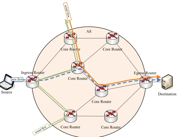
In order to provide QoS to an application or flow in a network, a group of mechanisms such as admission control, resource reservation, scheduling, classification, policing, or shaping may be used. AC, in particular, can be used to control the amount of traffic entering in a network. AC mechanisms were used in the Public Switched Telephone Networks (PSTN). When a call is to be established, the AC mechanism is performed and decides if the call is accepted (resources available in the network), or if the call is rejected (no resources available in the network for the call). In these networks the main objective of the AC is to help determine if the network has enough resources for the incoming request.

In packet switched IP networks, the AC is also used to provide QoS through Integrated Services (Intserv) [60] and Differentiated Services (Diffserv) [61] architectures. Intserv is based on per-flow reservations in the network to provide per-flow QoS guarantees. This approach requires maintenance of individual flow states in the routers, and its signaling complexity grows with the number of flows; here the AC is used to decide if new flows are or not accepted. Diffserv relies on packet markers, policing functions at the edge routers, and different per-hop behaviors at core routers to provide QoS to aggregated traffic; here the AC may not be used, but its deployment is recommended to control real-time traffic at the ingress node [62] (for instance, for traffic classified with an Expedited Forwarding Per-Hop-Behavior). Intserv and Diffserv implementations in the IP global network are not used since the Internet is composed of multiple AS with different network administrations. Thus, these implementations are only applied in a set of IP networks under a unique administration.