This is an Author's Accepted Manuscript of an article published as: ROSETA-PALMA, C. (2003) Joint Quantity/Quality Management of Groundwater. Environmental and Resource Economics, 26(1), 89-106 available online at: http://dx.doi.org/ 10.1023/A:1025681520509
Joint Quantity/Quality Management of
Groundwater
Catarina Roseta-Palma
∗Dep. Economia - ISCTE
Av. Forças Armadas
1649-026 Lisboa - Portugal
[email protected]
Abstract
Economic literature on groundwater management has traditionally been split into two areas: there are papers that evaluate different schemes of dy-namic aquifer management, considering that pumping costs vary with stock but ignoring water quality. On the other hand, there are papers that consider contamination problems caused by specific pollutants. This paper presents two alternative models for joint quantity-quality management, and it shows that existing models are in fact special cases of these. The framework is dynamic and considers both the stock of water quantity and a stock mea-sure of water quality. Optimal taxes are derived, and shown to be different from those in existing quantity-only or quality-only models. Implementation problems are briefly discussed.
Keywords: Groundwater, quantity-quality management, optimal taxes JEL classification: H23, Q15, Q25, Q28
1
Introduction
Aquifers have always been used as sources of water, and their importance in water management can be great. It is widely known that water as a resource needs to be managed beyond mere quantity allocations, since the quality of
the water is often decisive when determining how much of it will be used. Given the dynamic nature of groundwater, this means both the stock of water held by an aquifer and the stocks of whatever pollutants contaminate it are essential variables.1 Many existing aquifers, especially those in semi-arid regions where agricultural production is intense, present both scarcity problems (overdraft) and quality deterioration. In Portugal, for example, such is the case with some important aquifers in the South (Évora, Beja, Algarve).
Groundwater is usually exploited in a common property regime, in the sense that access is limited to owners of the land overlying the aquifers. This creates externalities since one unit of water extracted is no longer available to others and lowers the water table for everyone. Additional externalities are present because individual contamination affects all users. Furthermore, there are several reasons why the relationship between water pumping deci-sions and contamination cannot be ignored. First, the economic decision to pump is associated with the choice of polluting inputs. Second, the actual contamination that percolates to the aquifer also depends on how much wa-ter is applied on the surface. And finally, the quality of the wawa-ter may alwa-ter its productivity. Yet the bulk of existing economic literature treats these two aspects of groundwater management independently.
Evidently, common property solutions are always associated with lower levels of social welfare than what could be achieved under optimal manage-ment. Two interesting questions arise then: how big is this welfare loss and what can be done about it? The answer to the first question should allow decision makers to decide whether or not to intervene in the aquifer; if inter-vention is desirable, the answer to the second question should allow them to decide on the most appropriate type of policy instrument to apply. The size of the welfare loss brought about by common property arrangements is largely an empirical question. In water quantity management, a few studies exist, beginning with Gisser and Sanchez [5], although results vary somewhat (see Provencher [15] for a survey). However, for quality management, perhaps due to the negative impacts on public health often associated with contami-1Likewise, for surface water management quantity and quality should also be consid-ered jointly (see Costa [2]). However, the static framework adopted for surface water is inadequate for groundwater.
nation of aquifers, or because remediation programs tend to be difficult and expensive, the need for intervention is no longer an issue. Most countries already have maximum standards established for the most important pollu-tants (for instance, the US Clean Water Act, the EU Nitrates Directive EC 91/676) Although these requirements are not necessarily those that maxi-mize welfare, their existence establishes that intervention is warranted. So here the choice of policy instruments is the key issue.
In the quantitative management literature, policy recommendations in-clude water charges and water quotas which essentially lead users to repro-duce the pumping paths of central control (see Feinermann and Knapp [4], Neher [12]). A less interventionist strategy is described by Provencher [14], where users receive an endowment of tradable permits which they control over time. Typical pollution control literature also suggests variations on taxes or permits. Instruments can be targeted at actual discharges or at the inputs that cause them, which are easier to monitor and will be equally effi-cient as long as the pollution production function is known (see Griffin and Bromley [6]). Since complete information on pollution processes is frequently unavailable, incentives can take the form of penalties on deviations between observed and desirable discharges (Segerson [18]). Xepapadeas [22] presents such incentives for the case of a dynamic pollutant accumulation model with imperfect monitoring. Given implementation difficulties, there is also some work in the literature evaluating suboptimal pollution control instruments (see Shortle and Dunn [20], Larson et al. [9], Helfand and House [8], and Mapp et al. [11]).
This paper uses a dynamic resource management perspective to show how an optimal policy takes into account effects on water stock as well as on its quality. The cases in which it doesn’t are shown to be special cases of the joint management solution. In a model where an output is produced using water and another input, which then combine to cause pollution, the optimal taxes on groundwater extraction and on the polluting input are calculated assuming that the producers/users of the water are myopic. It is shown that taxes based on typical models of quantity-only or quality-only are in-efficient and may not even lead the common property aquifer in an optimal direction. Similar results are obtained when quality enters the problem as a
restriction instead of directly affecting productivity. Implementation prob-lems associated with optimal policies are briefly discussed, and an illustration is provided.
2
Why private pumpers do not maximise
wel-fare
The exploitation of a stock of groundwater is typically a problem of common property, since there is limited access to the resource. If each user is a profit maximising agent, there are a number of well known reasons for the inefficiency of the private solution.
First, the fact that there is a finite stock means that each unit that is extracted by one firm is no longer available to the others. Given that the only way to lay claim to a unit of groundwater is to pump it, there is little incentive to save water for later use, since other firms have the same access to the stock. Hence firms will pump an inefficiently large amount of groundwater. Moreover, pumping costs generally depend on the water table level, which means that as the groundwater stock is depleted, extraction costs rise. However, the individual user does not consider the detrimental effect of its pumping on other firms’ costs, so again there is an incentive to overpump. Finally, if the aquifer under consideration is susceptible of contamination resulting from users’ actions in the land overlying the aquifer, then additional externalities occur. Since each user will only consider his own polluting impact on the stock (or not even that one, if the agent behaves myopically), he has a motive to overpollute, imposing external costs on all other users of the water. Note that the presence of contamination implies that private agents will implement not only a suboptimal choice for water but also a suboptimal choice for contaminating actions (such as fertilizer or pesticide use). There is also less incentive to invest in groundwater protection and/or remediation programs.2
2Considering the presence of uncertainty would originate a risk externality (see Provencher and Burt [13]).
3
Joint quantity/quality model
Consider a dynamic, continuous time model of groundwater management for an aquifer with constant recharge, R. Assume that M identical firms exploit a single stock of groundwater, which contains Gt units of recoverable water and is characterised by a flat bottom and perpendicular sides. The water has a known level of quality, Ψ, which affects the profitability of water use. Worsening quality might be due to nitrates in the water, dissolved solids, trace metals, or any other relevant quality measure. All firms produce some good using water and another input with a production function y(gt, γt; Ψt), where gt is the amount of water used and γt is an input whose use creates pollution. The following properties are assumed:
• positive but diminishing marginal returns for both inputs: ∂y∂g, ∂y ∂γ > 0, ∂2y ∂g2, ∂2y ∂γ2 < 0 • complementarity of inputs: ∂g∂γ∂2y > 0
• positive effect of water quality on production:3 ∂y ∂Ψ > 0
• positive effect of water quality on marginal productivities of other in-puts: ∂g∂Ψ∂2y > 0, ∂γ∂Ψ∂2y > 0
The unit cost of groundwater extraction, denoted by c(Gt) is decreasing and convex). Labelling each firm’s extraction of groundwater gt, each firm’s net benefit at period t is given by:
pyy(gt, γt; Ψt)− c(Gt)gt− pγγ (1)
Considering a return coefficient of α, the groundwater stock behaves ac-cording to:
∂Gt
∂t ≡ ˙G =−M(1 − α)gt+ R (2)
3Examples of papers where water quality affects productivity are Letey and Dinar [10], Zeitouni and Dinar [25] and Dinar [3], although in those cases the relevant quality parameter is salinity which is not dependent on specific inputs.
Water quality will degrade as it receives contaminant loads, which origi-nate on the surface and percolate towards groundwater according to a pollu-tion producpollu-tion funcpollu-tion that depends on how much water is used and on the amount of polluting input, e(gt, γt), so that ∂g∂et > 0,
∂e
∂γt > 0and ∂2e
∂gt∂γt > 0.
Increasing amounts of water are assumed to increase pollution because wa-ter is a carrier for the pollutants. However, this effect could be negative, at least for some range of w, if other roles of water were considered, namely its complementarity with polluting inputs in the production of y (for instance, in agriculture, water allows plants to absorb nitrogen and phosphorus more efficiently decreasing the presence of these elements in topsoil) and its own dilution effect (if all the contaminant load is already being carried down, the addition of extra water will improve the quality of the leachates that reach the aquifer). Examples of pollution production functions for nitrates in agriculture can be found in Vickner et al. [21], Larson et al. [9], and Helfand and House [8]. Following the contamination literature (see Yadav [24] for nitrates, Anderson et al.[1] for pesticides), it is assumed that there is a constant natural decay rate for the pollutant, so that contamination would evolve according to:
˙
C = M e(gt, γt)− δCt (3)
A more realistic version of this equation would include delayed response ef-fects, as pollutants do not reach groundwater instantly. Note that if stock effects existed, they could enter the function through their impact on the decay rate, which might be more generally represented as δ(C, G).
The quality measure should be defined so that it decreases with contam-ination. One possibility is to define quality as the difference between the maximum possible stock of contaminant the aquifer can take and its actual presence, Ψt = Cmax− Ct, implying that the associated quality function is:4
˙
Ψ = δ(Ψmax− Ψt)− Me(gt, γt) (4)
4This specification is equivalent to Ψ = −C. The additional term simply ensures that Ψ is a positive value. An alternative specification is Ψ = 1
3.1
Optimal vs. Common Property Management
The problem facing a water planner would be to choose optimal extraction paths and input use for each firm, i.e. to determine which paths maximise the total present value of net revenues. It is assumed that there are no environmental externalities, otherwise these would have to be considered as well.
Formally, the water planner’s problem is:
max gt ∞ Z 0 M [pyy(gt, γt; Ψt)− c(Gt)gt− pγγ] e−ρtdt (5)
subject to equations 2 and 4 and to non-negativity restrictions and/or maxi-mum levels for Gt,and Ψt,as well as initial conditions G0 = Gand Ψ0 = Ψ. ρ is the appropriate discount rate, which is assumed to be constant. This is a typical optimal control problem. The current value Hamiltonean is:
H = M (pyy(gt, γt; Ψt)− c(Gt)gt− pγγ) + (6) λt(−M(1 − α)gt+ R) + βt(δ(Ψmax− Ψ) − Me(gt, γt))
The results obtained from first order conditions can be summarised as:5
py ∂y ∂gt = c(Gt) + λt(1− α) + βt ∂e ∂gt (7) py ∂y ∂γt = pγ+ βt ∂e ∂γt (8) ˙λ = ρλt+ M ∂c ∂Gt gt (9) ˙β = (ρ + δ) βt− Mpy ∂y ∂Ψt (10) The first equation represents the usual optimality result that marginal benefit in each period will be equal to total marginal extraction cost, which is the sum of three terms: actual extraction cost, opportunity cost of removing 5These are necessary and sufficient if the Hamiltonean function is jointly concave in g, γ, G and Ψ or if the maximized Hamiltonean is concave in G, Ψ. At this point concavity requirements are assumed to be satisfied. However, in typical empirical applications such conditions may not hold. See illustration.
one unit of water from the ground (reflecting the future impact on profits for all firms), and an additional cost due to the impact of extraction water, which is applied then returns with contaminants, on water quality. The second equation shows an equivalent result for the other input: marginal benefit is equal to actual marginal cost plus the cost of quality deterioration. The third and fourth equations describe the behaviour of the shadow prices of quantity and quality, respectively. Note that the evolution of β reflects the positive impact of quality on profits as well as the regeneration rate.
In the presence of a positive recharge and a natural regeneration rate, it is possible to have a steady state with positive pumping and positive discharges, for which: G = 0, ˙˙ Ψ = 0, ˙λ = 0 and ˙β = 0. These yield, respectively (variables are at their steady state values):
g = R (1− α)M (11) Ψ = Ψmax− M e(g, γ) δ (12) λ = −M ∂c ∂Gg ρ (13) β = M py ∂y ∂Ψ ρ + δ (14)
From these equations it can be noted that at the steady state pumping is exogenous (equation 11), quality will be higher for lower levels of pollution (equation 12), the shadow price of water in the ground will be higher for lower levels of stock (equation 13), and the shadow price of water quality will be higher when the impact of quality on production is higher (equation 14). Note that in the special case where unit cost is approximately constant,
∂c
∂G = 0, and the constraint gt ≤ Gt is not binding, which might happen in very large aquifers with sizable recharges (implying a relatively stable water stock), a quality-only model could be appropriate, while if ∂Ψ∂y = 0 a quantity-only model is appropriate.
In a common property situation, if the users of groundwater behave my-opically (MB), they choose gt and γt by individually maximizing profit, ig-noring the dynamic evolution of G and Ψ.6The relevant first order conditions 6For other types of common property equilibrium see Provencher and Burt [13], Xepa-padeas [23], Rubio [17], and the references therein.
are: py ∂y ∂gt = c(Gt) (15) py ∂y ∂γt = pγ (16)
Although optimal management could be expected to achieve a larger aquifer of better quality, it can be shown through comparison of 15 and 16 with 7 and 8 that the common property solution attains a steady state which might have higher or lower quantity, although it will certainly have better quality. The possibility that intervention worsens one of the objectives cannot be disregarded. This result can be explained by noting that higher quality water is more productive, so that it may be efficient to pump more of it and reach a steady state where there is less water. It can also be shown, using equation 12, that myopic users will apply more of the polluting input than would be efficient at the steady state, which is the anticipated result.7
3.2
Taxes
One of the ways for the common property arrangement to replicate the optimal solution is to impose a set of input taxes on users so that their choice of both extracted water and applied contaminants reflects society’s marginal costs instead of their own. In this case, that would require Ttg = (1−α)λt+ βt ∂e ∂gt and T γ t = βt ∂e
∂γt.Naturally, the tax on water reflects both its
scarcity cost and its role in groundwater contamination. Moreover, although the tax on the polluting input only reflects its impact on quality (as γ does not affect G directly), it should be stressed that optimal values of βtand ∂γ∂et
will also depend on the path of water extraction.
The tax schedule presented above would bring myopic users to optimal levels of gt and γt for all t, and thus maximize social welfare. A theoreti-cally equivalent alternative would be to issue permits for the use of water as well as for the other input. The market price of water permits would reflect 7Different results are obtained in Palma [16] with different assumptions on the qual-ity function, namely that ∂Ψ∂f > 0. This disparity highlights the importance of accurately representing the physical properties of the aquifer and its reactions with specific contam-inants.
both water’s relative scarcity and its effect on quality once applied. Conven-tional management arrangements, where only quantity or only quality are controlled, are presented subsequently to emphasize their inefficiency.
Consider first the problem of the “Stock Manager”, who takes quality parameters as given and seeks to impose a tax on extracted water. The first order conditions for extraction yield:
py ∂y ∂gt = c(Gt) + λt(1− α) (17) ˙λ = ρλt+ M ∂c ∂Gt gt (18)
If the manager takes γ and Ψ as given and sets a tax of λt(1− α), not only is this solution different from the optimal one, it may also lead the aquifer towards a steady state that is even further from its optimal state (if it was the case that GM B > GOP T). With the tax, first order conditions for the user’s problem are 16 (which the regulator ignores) and 17. The imposition of this tax will alter his decisions on gt and γt.However, in the steady state extraction returns to its usual exogenous value, so that Ψ and γ must also return to their previous steady state levels (by 16 marginal revenue of γ is constant at all times as long as the prices of output and γ remain constant). Thus equation 17 implies that the new steady state stock is higher than the myopic case. The selected tax is inefficient because it doesn’t consider water’s role as a contaminating vector. However, note that this does not mean the tax is always lower than the optimal one, since λtas calculated by the “Stock Manager” is different.
Now consider the problem of the “Contamination Regulator”, who will decide what taxes to charge on contaminating inputs, considering that water is pumped at a constant price (or equivalently, that G is taken as given). The choice will be characterized by:
py ∂y ∂gt = c(Gt) + β ∂e ∂gt (19) py ∂y ∂γt = pγ + β ∂e ∂γt (20) ˙β = (ρ + δ) β − Mpy ∂y ∂Ψ (21)
Thus chosen taxes will again not coincide with the optimal ones. In this case not much can be said on the evolution of variables after taxes are set. Nevertheless, it is clear that the optimal stationary solution will never be achieved because with similar values of γ, Ψ, g, and G, equations 7 and 19 cannot both be valid. Moreover, if both types of regulators exist and taxes are set separately, the optimal solution will generally still not be achieved, and results will depend on what sort of strategy each of the regulators follows. This may have important implications both for policy and for institutional design.
4
Minimum quality requirements
Previous sections assumed that the main reason for controlling groundwater pollution was its impact on the productivity of applied water, since it was an input in the production of some other good. However, the observed ne-cessity for pollution control has often arisen from a different reason. Water contamination brings other damages to society, either directly (public supply of drinking water) or indirectly (deterioration of ecosystems associated with aquifers). To include these effects in the previous model, it would be sufficient to come up with a water damage function for society, add it to the objective function of the model, and proceed with maximization as usual, calculating optimal taxes that would induce polluters to act efficiently.8 This could eas-ily be done if the water damage function was known. Since it generally isn’t, an alternative is to impose existing quality requirements on the management problem.9
In what follows it will be assumed that quality does not affect production. It will be shown that even in this case, the existence of a restriction on Ψ means that optimal policy must again consider stock effects on quantity and quality jointly. The management problem is similar to problem 5 with an additional restriction: Ψt≥ Ψ, where Ψ is the minimum permissible quality 8See Yadav [24]. To adequately choose the optimal quality level would require infor-mation on the damages brought about by increased pollution concentration, in terms of health, environmental or amenity effects.
9Another alternative would be to consider a cost function associated with treating water of quality Ψ whenever Ψ≤ Ψ.
level. Associating a multiplier function, η(t), with the restriction, yields:10 py ∂y ∂gt = c(Gt) + λt(1− α) + βt ∂e ∂gt (22) py ∂y ∂γt = pγ+ βt ∂e ∂γt (23) ˙λ = ρλt+ M ∂c ∂Gt gt (24) ˙β = (ρ + δ) βt− ηt (25) ηt≥ 0; ηt(Ψt− Ψ) = 0 (26)
These look exactly the same as in the case where productivity of water de-pended on its quality, except the behaviour of quality’s shadow price is ex-plained by a different reason: the opportunity cost of diminishing quality no longer reflects its impact on profit, but it incorporates the effect of the restriction. Just as before, optimal policies include effects both on quality and on quantity. If the restriction is never binding (ie. quality is never a problem), then ηt = 0 ∀t, implying that βt = 0, so that only quantity actu-ally needs to be managed. In this case, typical quantity-only water resource models would be sufficient.
On the other hand, it can be shown that the restriction will be binding at the steady state if Ψ is higher than ΨM B. To show this, note that if Ψ was not binding at the steady state, the stationary value of β would be zero, so that by 23 the chosen value of γ would be the myopic one. However, with the same g and γ, steady state quality would be the same as that of the myopic case, so that Ψ must in fact be binding. Thus, if an aquifer that is being exploited under the common property regime has a quality problem, better management of water quantity will not solve the quality problem.
The fact that Ψ is binding at the steady state may allow policy makers to look at the problem in a slightly different way. Since Ψ can be used to calculate the corresponding steady state stock G, using equation 22 and replacing λ with its steady state value, there is a combination (Ψ, G) which can be used as the joint management goal. Thus the cost-effectiveness of alternative instruments (especially suboptimal ones) in reaching this goal 10Additionally, eventual discontinuities of the co-state variables would have to be anal-ysed. See for example Seierstad and Sydsaeter [19].
can be evaluated. The main difference for the dynamic case is that the quality restriction may not be achievable as soon as it is imposed, so that a few periods will lapse before the target is reached (the choice of actions to undertake during this period may consider criteria related to the speed of adjustment associated with alternative policies). The illustration in section 5 includes such considerations.
Although it is theoretically easy to calculate a set of optimal taxes that solve the groundwater management problem, the implementation of such a scheme is quite a different matter. Not only might there be monitoring problems, but in reality, the M users of the aquifer will generally not be all alike, either because their production processes are different or because the pollution functions are different. Such disparities do not complicate the theoretical model much, since optimal taxes will look the same except that there are M sets of individual ones. However, implications for implementation are huge. Furthermore, if different users have different quality requirements, the dynamics of the model might imply that some users abandon groundwater extraction altogether as its quality worsens.
Helfand [7] and Helfand and House [8] analyse problems with input-based policies and compare them to emissions-based ones, noting that the latter are more difficult to implement in the nonpoint pollution case due to the frequent unobservability of emissions. The implementation of emissions taxes is even less attractive in the joint quantity/quality dynamic model because water has to be taxed anyway due to the scarcity problem. These two papers, as well as Larson et al. [9], deal specifically with the issue of suboptimal input-based instruments, such as uniform taxes for different users or single-input taxation. Additional inefficiencies of simpler schemes might appear in the dynamic case, since optimal tax levels require continuous adjustment to reflect changing scarcity and quality costs.
5
Illustration
In this section an application in the management of a contaminated aquifer is developed.11 This example was constructed used real, estimated functions 11Many grateful thanks to Ana Balcão Reis, Duarte Brito, and especially António An-tunes; without their input this illustration would have been impossible.
from several sources, namely Yadav [24] (contamination function), Larson et. al [9] (production and emissions functions), as well as Zeitouni and Dinar [25] and Feinermann and Knapp [4] (some aquifer characteristics, pumping costs). It analyses agricultural production using nitrates and irrigated wa-ter under myopic behaviour of farmers and compares it to a quantitatively optimal solution. Then a minimum quality requirement (or rather, a maxi-mum concentration limit) is imposed and the optimal taxes that would lead the common property equilibrium to an efficient solution that satisfies the restriction are identified.
The notation is slightly different from that of previous sections because empirical applications use pumping lift and pollutant concentration, rather than the more theoretical variables G and Ψ. However, there is one to one correspondence between lift and stock, on one hand, and quality and concen-tration, on the other. Moreover, the profit maximizations will be undertaken per ha instead of per farmer.
The evolution of lift, L (which represents the distance between the land surface and the water level) can be represented by:
˙
L = (1− α)g T
− R
AS (27)
where gT is the total water used (gT is the sum for the entire area farmed of the per ha water applied) , A is aquifer area and S is the specific yield. Pollutant concentration will be assumed to evolve according to:
˙
C = ηN O3− δCt
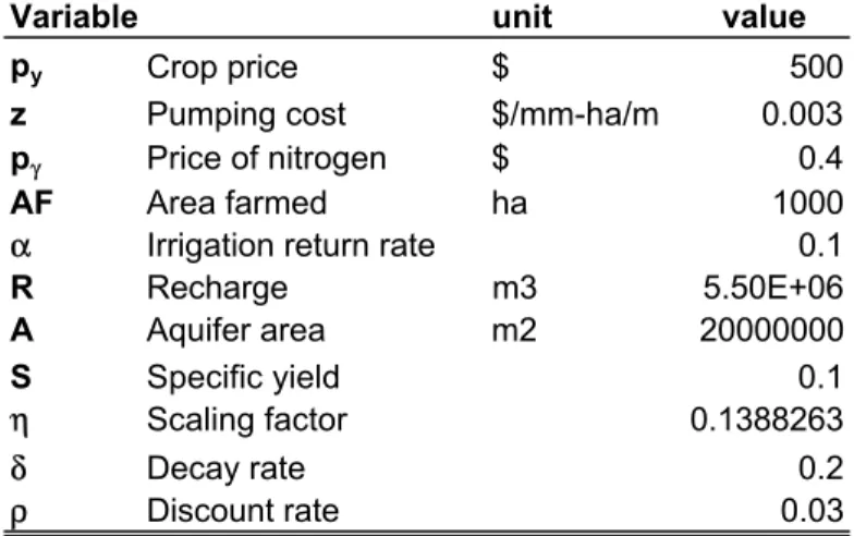
where N O3 is emitted nitrates as a function of applied nitrogen and water, and η is a scaling term. The production function is quadratic and unit pumping cost is linear in lift. Tables 1, 2 and 3 present parameter values and clarify physical units.
Starting with the aquifer in a “pristine” condition (L(0) = 1, C(0) = 0) and solving the problem without considering any quality restrictions, the appropriate first order conditions (see equations 15 and 16) yield the my-opic behaviour paths for lift, water and nitrates. At the steady state, γ = 88.953, .g = 611.08, and Lt = 101.05. Furthermore, the aquifer will be con-taminated as soon as 3 years after initial exploration, and pollutant concen-tration will reach a steady state value of C = 62.17 (concenconcen-tration worsens
MODEL
Table 1 Table 2
Variable unit value Production function
py Crop price $ 500 Y=a+bγ+cg+dγg+eγ
2+fg2
z Pumping cost $/mm-ha/m 0.003 a 2.52
pγ Price of nitrogen $ 0.4 b 0.000535
AF Area farmed ha 1000 c 0.00151
α Irrigation return rate 0.1 d 0.000002
R Recharge m3 5.50E+06 e -5.38E-06
A Aquifer area m2 20000000 f -8.85E-07
S Specific yield 0.1
η Scaling factor 0.1388263
δ Decay rate 0.2 Table 3
ρ Discount rate 0.03 Leaching function NO3=h+iγ+jg+kγg h -26.06 i -0.152 j 0.158 k 0.0006
even more in the initial periods, but as the aquifer table becomes lower, pumping and fertilizer applications decrease until C is stable. See Figure 2, thin line)
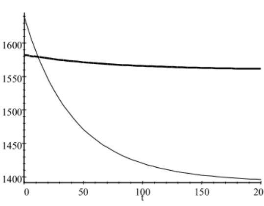
In contrast, optimal quantitative management paths (thick lines on Fig-ures 1-3) are derived from equations 7 and 8.12 At the steady state, L = 9.382, g = 611.1 and γ = 88.955. The steady state is achieved asymptotically and the present value of total welfare losses from common property man-agement amounts to a negligible 1461 $/ha (which is approximately 2.8% of optimal welfare). The reason is that lift is small in the first years of pumping, so costs are similar; yet more nitrogen and water are applied in the common property case, making revenue higher (see Figure 3). Because of discount-ing, these first periods weigh heavily on the final outcome. Only after some periods of aquifer overexploitation does lift decrease sufficiently to make this effect disappear, thereby yielding lower profits for common property than those of the efficient case. .
This looks like one of those aquifers for which quantity only management does not bring great welfare gains, in the line of Gisser and Sanchez [5] and others. However, considering current restrictions for maximum allowable concentration of nitrates in the water of 50 mg/l, this aquifer clearly has a quality problem. How might that problem be solved in our example? The actual answer depends on when the restriction is imposed. It could be imposed as soon as concentration hits 50 mg/l, which will happen between year 3 and 4, but this would imply the aquifer would never be overpolluted. More realistically, it can be assumed that agents were already overpolluting the aquifer before some measure is attempted. For ease of exposition, take as a starting point the common property steady state described above. If nitrogen applications are forbidden until the standard is reached (which has a much lower cost than forbidding cultivation altogether), it will take between three and four years to do so. Farmers could be compensated for their profit losses, which would amount to 52.8 $/ha for the whole period. At that point, L = 99.477.and C = 50. After that time, a set of quantity-quality 12Due to the linearity of pumping costs these are not sufficient. However, the system of differential equations defined by the first order conditions and the transition equation for L is linear, so it can be solved and there is only one stable path that satisfies first order conditions.
Comparison of optimal and myopic behaviour paths
Figure 1. Pumping Lift (m) Figure 2. Concentration (mg/l)
0 20 40 60 80 100 50 100t 150 200 0 20 40 60 80 100 120 50 100t 150 200
Figure 3. Current value profits ($/ha)
1400 1450 1500 1550 1600 0 50 100t 150 200
taxes would be imposed both on water and fertilizer. The relevant system of differential equations cannot be solved analytically, and it does not have an interior steady state. A solution was obtained using MATLAB.
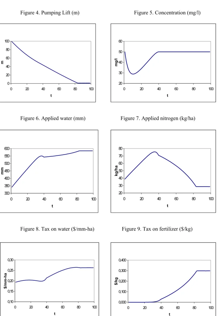
Optimal paths for lift, water, fertilizer, and concentration are presented in Figures 4-7. Concentration actually falls below its maximum allowable value for the first few periods, where the incorporation of the “quantitative” opportunity cost leads to much lower water use than that of the MB steady state. Then, as lift decreases, pumping and fertilizer increase, until the con-centration limit is reached again. The average tax on water is 0.23 $/mm-ha and that on fertilizer is 0.11 $/kg (although it is zero as long as C < 50 mg/l). See Figures 8-9. The difference in steady state welfare between the optimal case with and without the quality restriction is a paltry 1$/ha per year. That is the cost the government is imposing on society by requiring a minimum quality level.
6
Conclusion
Economic literature on groundwater management has traditionally been split into two areas: on the one hand there are papers that evaluate different schemes of dynamic aquifer management, considering that pumping costs vary with stock but ignoring water quality. On the other hand there are papers that consider contamination problems caused by specific pollutants. Among these, only a few are dynamic in nature, and only a few include water in their estimation of pollution functions. Yet even those consider that water can always be obtained at a constant price, which does not reflect changes in pumping costs. This paper presents two alternative models for joint quality-quantity management, and it shows that existing models are in fact special cases of these. Thus existing models continue to be adequate when aquifers conform to those special cases, but are in general not applicable to the more complex problem of managing an aquifer when both quantity and quality are relevant variables.
Using assumptions from both areas of the literature, the paper shows that when quality and quantity of aquifers are important, optimal policies must reflect the relationship between them. The main features used in the
Incorporating a quality restriction
Figure 4. Pumping Lift (m) Figure 5. Concentration (mg/l)
0 20 40 60 80 100 0 20 40 60 80 10 t m 0 20 30 40 50 60 0 20 40 60 80 10 t mg/l 0
Figure 6. Applied water (mm) Figure 7. Applied nitrogen (kg/ha)
300 350 400 450 500 550 600 0 20 40 60 80 10 t mm 0 20 30 40 50 60 70 80 0 20 40 60 80 10 t kg /ha 0
Figure 8. Tax on water ($/mm-ha) Figure 9. Tax on fertilizer ($/kg)
0,10 0,15 0,20 0,25 0,30 $/mm-ha 0,000 0,100 0,200 0,300 0,400 $/kg
characterization of production and pollution functions draw heavily on agri-cultural contamination literature. Furthermore, since the myopic behaviour hypothesis is adopted, the model is particularly suitable to analyse aquifers exploited by a large number of agricultural producers that are relatively small and face identical physical conditions. Nonetheless, the same frame-work could be adapted to other types of common property behaviour as well as to different uses for the water.
The theoretical model furnishes some interesting insights, but those focus mainly on steady state characteristics. Specific functions for production, pollution production, and pumping costs are required for a more complete analysis of system properties. Ultimately, the usefulness of models such as these hinges on empirical work, not only to check which variable paths lead to which steady states, but also to evaluate welfare losses from different, non-optimal situations, so that unregulated common property or regulated common property with suboptimal instruments can be appraised. That is the purpose of the illustration presented.
Other important areas have been left out in the analysis. Paramount among these are the choice between surface water and groundwater in con-junctive use models with quality differences, and the incorporation of uncer-tainty. When quality is an issue surface water and groundwater can no longer be considered perfect substitutes in production. Moreover, available surface water is not constant throughout time (in semi-arid climates great variability is observed both within the year and between different years). The inher-ent uncertainty in hydrological variables could have important implications. In fact, there is inherent uncertainty both in water availability (especially in semi-arid climates) and in many aquifer pollution processes. Further research should be dedicated to these aspects.
References
[1] G. Anderson, J. Opaluch and W.M. Sullivan, Nonpoint Agricultural Pollution: Pesticide Contamination of Groundwater Supplies, American Journal of Agricultural Economics 67, 1238-1246 (1985)
[2] L. Costa, Control of Water Use in Northwest Portugal, Phd dissertation, Dept. Economics, University of Arizona (2001)
[3] A. Dinar, Impact of energy cost and water resource availability on agri-culture and groundwater quality in California, Resource and Energy Eco-nomics 16, 47-66 (1994)
[4] E. Feinermann, K.C. Knapp, Benefits from Groundwater Management: Magnitude, Sensitivity, and Distribution, American Journal of Agricul-tural Economics 65, 703-710 (1983)
[5] M. Gisser and D.A. Sanchez, Competition versus Optimal Control in Groundwater Pumping, Water Resources Research 16, 638-642 (1980) [6] R. C. Griffin and D. W. Bromley, Agricultural Runoff as a Nonpoint
Ex-ternality: A Theoretical Development, American Journal of Agricultural Economics 64, 547-552 (1982)
[7] G. Helfand, Controlling Inputs to Control Pollution: When Will It Work?, AERE Newsletter, vol 19, No.2 (1999)
[8] G.Helfand and B.House, Regulating Nonpoint Source Pollution Under Heterogeneous Conditions, American Journal of Agricultural Economics 77, 1024-1032 (1995)
[9] D. Larson, G. Helfand and B. House, Second-Best Tax Policies to Reduce Nonpoint Source Pollution, American Journal of Agricultural Economics 78, 1108-1117 (1996)
[10] J.Letey and A. Dinar Simulated Crop-Water Production Functions for Several Crops When Irrigated with Saline Waters, Hilgardia 54, 1, 1-32 (1986)
[11] H.P.Mapp, D.J. Bernardo, G.J. Sabbagh, S. Geleta and K.B. Watkins, Economic and Environmental Impacts of Limiting Nitrogen Use to Pro-tect Water Quality: A Stochastic Regional Analysis, American Journal of Agricultural Economics, 76, 889-903 (1994)
[12] P.Neher, “Natural Resource Economics - Conservation and Exploita-tion”, Cambridge University Press (1990)
[13] B. Provencher and O.Burt, The Externalities Associated with the Com-mon Property Exploitation of Groundwater, Journal of Environmental Economics and Management, 24, 139-158 (1993)
[14] B. Provencher, A Private Property Rights Regime to Replenish a Groundwater Aquifer, Land Economics, 69 (4), 325-40 (1993)
[15] B. Provencher, Issues in the Conjunctive Use of Surface Water and Groundwater, in “The Handbook of Environmental Economics” (D.Bromley, Ed.), Blackwell (1995)
[16] C.Roseta-Palma, Groundwater Management when Water Quality is Endogenous, Journal of Environmental Economics and Management, forthcoming (2002)
[17] S.Rubio, “Strategic behavior and efficiency in the common property ex-traction of groundwater”, presented at the Symposium on Water Man-agement - Efficiency, Equity and Policy, at the University of Cyprus, Nicosia, September 22-24 (2000)
[18] K.Segerson, Uncertainty and Incentives for Nonpoint Pollution Control, Journal of Environmental Economics and Management, 15, 87-98 (1988) [19] A.Seierstad and K.Sydsaeter, “Optimal Control Theory with Economic
Applications” North-Holland (1987)
[20] J.Shortle and J.Dunn, The Relative Efficiency of Agricultural Source Water Pollution Control Policies, American Journal of Agricultural Eco-nomics, 68, 668-677 (1986)
[21] S. Vickner, D. Hoag, W.M. Frasier and J. Ascough II, A Dynamic Eco-nomic Analysis of Nitrate Leaching in Corn Production under Nonuni-form Irrigation Conditions, American Journal of Agricultural Economics 80, 397-408 (1998)
[22] A.P. Xepapadeas, Environmental Policy Design and Dynamic Nonpoint-Source Pollution, Journal of Environmental Economics and Manage-ment 23, 22-39 (1992)
[23] A.P.Xepapadeas, Managing common-access resources under production externalities in “Economic Policy for the Environment and Natural Re-sources”, ed. A.Xepapadeas, Edward Elgar (1996)
[24] S. Yadav, Dynamic Optimization of Nitrogen Use When Groundwater Contamination Is Internalized at the Standard in the Long Run, Amer-ican Journal of Agricultural Economics 79, 931-945 (1997)
[25] N. Zeitouni and A.Dinar, Mitigating Negative Water Quality and Qual-ity Externalities by Joint Management of Adjacent Aquifers, Environ-mental and Resource Economics 9, 1-20 (1997)