Modeling the reverse segregation of reinforcements in functionally graded composites by the longitudinal casting method

(1)

João Oliveira Cardoso

Licenciado em Ciências da Engenharia de Materiais

Modeling the reverse segregation of reinforcements

in functionally graded composites by the

longitudinal casting method

Dissertação para obtenção do Grau de Mestre em Engenharia de Materiais

Orientador: Professor Doutor Alexandre José da Costa Velhinho,

Professor Auxiliar, FCT/UNL

Júri:

Presidente: Professor Doutor João Paulo Miranda Ribeiro Borges Arguente(s): Professor Doutor Rui Jorge Cordeiro Silva

Vogal(ais): Professor Doutor Alexandre José da Costa Velhinho

(2)

(3)

(4)

(5)

i “Copyright” João Oliveira Cardoso, Faculdade de Ciências e Tecnologia, Universidade Nova de Lisboa.

A Faculdade de Ciências e Tecnologia e a Universidade Nova de Lisboa têm o direito,

perpétuo e sem limites geográficos, de arquivar e publicar esta dissertação através de exemplares impressos reproduzidos em papel ou de forma digital, ou por qualquer outro meio conhecido ou

que venha a ser inventado, e de a divulgar através de repositórios científicos e de admitir a sua

(6)

(7)

iii

Acknowledgments

For all his support, patience and knowledge provided, I would like to thank my advisor,

professor Alexandre Velhinho. I am very happy to have had the opportunity to work with him

and look forward to continue in the future.

Secondly, I’d like to thank professor Pedro Medeiros, not only for his help with the com-puter provided for the simulations ran in this dissertation, but also for his help in my previous

work.

I would like to thank all my teachers during my degree, for their knowledge transmitted,

their kindness and everything they’ve done. It has truly been a blessing to have such great teachers

as my guides.

I would like to thank my faculty and everyone in it, they housed me for all these years

during my studies, and before that in Clubemath; in the same note, I would like to give a special

thanks to my dear professor Nelson Chibeles, a true gem of a person and teacher.

I would like to thank all my friends; you guys give life that extra sweetness and make some of the worst days into the best of moments. If there’s anything you need from me in the future, I’m here.

To my family, I’d like to thank all of them for their support, and for giving me the oppor-tunity to follow my studies, without them, I literally wouldn’t be here. A special mention to my parents, for helping me in this and all my journeys.

(8)

(9)

v

Resumo

Nesta dissertação foi simulada a produção de um compósito de matriz metálica com

gradi-ente de funcionalidade de Al/SiC, fabricado usando o método de fundição centrífuga longitudinal. Este método permite a produção de geometrias que outras variantes da fundição centrífuga não

permitem, tornando-o num método bastante vantajoso. Contudo, a fundição centrífuga

longitudi-nal carece de atenção por parte da literatura, nomeadamente relativo aos fenómenos de segrega-ção: inversa, dimensional e transversa.

Desenvolveu-se um código em MATLAB para o estudo da segregação inversa utilizando

o método das diferenças finitas com base numa malha estática. Deste estudo foi possível observar a relação entre a temperatura de vazamento e a distribuição final de partículas. Uma simulação

adicional foi feita considerando uma distribuição de partículas variado visando estudar

breve-mente o efeito da segregação dimensional.

(10)

(11)

vii

Abstract

In this dissertation, we simulate the production of an Al/SiC functionally graded metal

ma-trix composite, made using the process of longitudinal centrifugal casting. This specific method-ology allows the production of geometries that aren’t possible with other variants of the

centrifu-gal casting method, making it highly desirable; however, the longitudinal variant has not attracted

a wide attention in the literature, namely in regards to the phenomena of reverse, dimensional and transverse segregation.

A MATLAB code was developed to study the effects of reverse segregation; a fixed grid

finite difference method was used for this which resulted in the study of the relation between starting casting temperatures and final particle distributions. An additional simulation was made

considering a varied particle distribution to briefly study dimensional segregation.

(12)

(13)

ix

List of Figures

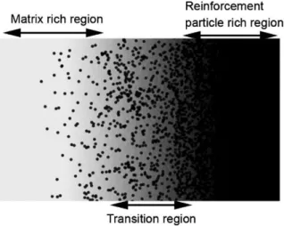
Figure 1 – Schematic illustration of a FGMMC with continuously graded microstructure.

Adapted from [2] ... 1

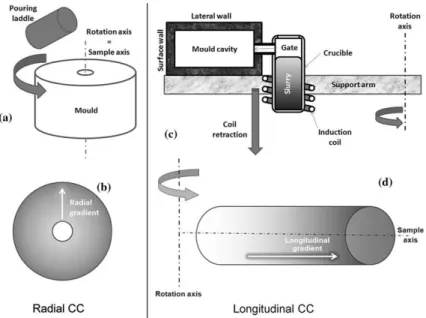
Figure 2 – Illustration of centrifugal casting. a) RCC furnace; b) gradient orientation in a FGMMC processed by RCC; c) LCC furnace; d) gradient orientation in a FGMMC processed by LCC. Adapted from [9]... 2

Figure 3 – FDM stencil for the heat equation using the Crank-Nicolson method. Adapted from [22] ... 3

Figure 4 – Particle area fraction profile for FGMMC cast by LCC of Al/SiC. a) Spin-up time of 5s; b) Spin-up time of 17s. Dv is the mean particle size; A, I, K, B, J, L were experiments made; 0 is the furthest point from the centrifugal axis. Adapted from [9] ... 4

Figure 5 – Mean particle diameter longitudinal profile. Adapted from [9] ... 5

Figure 6 – Transverse segregation. Adapted from [9] ... 5

Figure 7 – Particle Movement. Adapted from [16] ... 7

Figure 8 – Particle movement ... 8

Figure 9 – Enthalpy in function of temperature. Adapted from [23] ... 11

Figure 10 – Percentage surface for particles along the 20mm height. This is a result of experiment A ... 17

Figure 11 – Percentage surface for particles along the 20mm height. This is a result of experiment B ... 18

Figure 12 – Side-view of percentage surface for particles along the 20mm height. This is a result of experiment A ... 18

Figure 13 – Percentage surface comparison between experiment A and B. ... 19

Figure 14 – Percentage surface for particles along the 20mm height. This is a result of experiment C. ... 20

Figure 15 – Side-view of percentage surface for particles along the 20mm height. This result is of experiment C. ... 20

(16)

(17)

xiii

List of Tables

Table 1 –FDM coefficient calculation example for the unidimensional normalized heat equation

... 3

Table 2 –Coefficients’ position. ... 10

Table 3 – Explicit method convergence ... 13

Table 4 – Different parameters used ... 14

(18)

(19)

xv

List of Abbreviations, Acronyms and Symbols

Abbreviations and Acronyms:

Al – Aluminum

CC – Centrifugal casting

FDM – Finite difference method

FEM – Finite element method

FGM – Functionally graded materials

FGMMC – Functionally graded metal matrix composites

FVM – Finite volume method

J – Coefficient of the cell in study

J- – Coefficient of the previous cell in study, regarding the x-coordinates

J+ – Coefficient of the next cell in study, regarding the x-coordinates

K- – Coefficient of the previous cell in study, regarding the y-coordinates

K+ – Coefficient of the next cell in study, regarding the y-coordinates

L- – Coefficient of the previous cell in study, regarding the z-coordinates

L+ – Coefficient of the next cell in study, regarding the z-coordinates

LCC – Longitudinal centrifugal casting

M –Heat Equations’ coefficient matrix

RCC – Radial centrifugal casting

rpm – Rotations per minute

S – Position of interest in the M matrix

SiC – Silicon Carbide

TOL – Tolerance

TRM – Temperature recovery method

(20)

〈𝑎〉 – Average value of 𝑎

∆(x,y,z)– Cell size in the x, y or z direction in m

∆t– Time step

µl – Aluminum melt viscosity in kg/m s

Cp– Specific heat in J/kg K d – Particle size

Dv – Mean particle size in µm

H– Enthalpy in J/kg

jT–Fourier’s Law for diffusive heat flux

K – Thermal conductivity in W/m K

L– Latent heat of fusion in J/kg

R – Distance from the rotational center and the particle

T – Temperature in K

Te– Mold temperature in K

Tm– Melting point of Al in K

tmax – Spin-up-time in s

v– Velocity in m/s

ε– Phase fraction in V/V

ρ – Density in Kg/m3

ω– Angular velocity in rad/s-1

Subscripts:

→V– Entering the current control volume j, k, l– x, y, z components

L – Liquid phase

P– Particle phase

S– Solid phase

V→ – Exiting the current control volume

(21)

xvii t– Current time step

(22)

(23)

1

1 Introduction

Centrifugal casting (CC) is a technique that can be used in the production of functionally

graded metal matrix composites (FGMMC), a type of functionally graded materials (FGM). How-ever, CC may be obtained with two distinct methodologies: longitudinal centrifugal casting

(LCC) and radial centrifugal casting (RCC). LCC allows for more varied geometries to be

pro-duced but is not as much used as RCC because RCC is much easier to study and implement, despite its restrictions. We expect this work to be a further contribution to the production of LCC

FGMMC.

1.1 FGM and FGMMC

FGM are an advanced class of materials whose properties vary along at least one axis. Although very ancient, this concept has attracted materials scientists' attention after Japan’s space plane project in the mid 1980’s, it was afterwards popularized in the rest of the world. The idea behind FGMs is to have a property gradient along an axis. In the case of a composite, by mixing

two (or more) materials in a single matrix/reinforcement relation we can have the functionality gradient while avoiding interface problems [1]. Within the category of FGM, we have FGMMC,

composites (typically) made from metal and ceramic constituents (Figure 1).

There are several methods to produce FGMMC: infiltration, sedimentation/settling,

cen-trifugal casting, sequential casting, spray casting, powder metallurgy, slurry casting, and several deposition techniques [2]–[6]. Within all casting techniques two of them, RCC and LCC (Figure

2), allow the production of materials with better properties than the rest, namely: a denser

struc-ture, reduced porosity, grains radially oriented giving superior strength, fracture toughness and Figure 1 – Schematic illustration of a FGMMC

with continuously graded microstructure.

(24)

corrosion resistance; these properties make centrifugal casting the most sought process for the

production of functionally graded components [2].

RCC has already been extensively studied and is the major method used to produce FGMMC [2], but is limited to the fabrication of radial geometries parts: tubes, poles, beams,

pipes, etc... LCC, on the other hand, allows for more complex shapes but isn’t as studied as its radial counterpart. Designing parts using either technique is a complex problem to solve since the

equations associated with advection (particle displacement), temperature equilibrium and

solidi-fication are non-linear and inter-dependent, making numerical methods not only appropriate but also a necessity. Luckily in our modern age, computers have become powerful and common,

making such calculations possible in viable amount of time.

1.2 Modeling

Numerical methods have been around for a long time; with the invention of the computer

their use was increased. Recently, with the ever-increasing power of day to day computers, nu-merical methods have become popularized and of quick and simple access. Three methods are

nowadays available: Finite element method (FEM), finite volume method (FVM) and finite

dif-ference method (FDM). The first being one of the most popular and the last one of the simplest. The FDM is a fixed grid technique with a defined mesh (amount of nodes in a grid and their

arrangement), it qualifies as the best method for numerically solving partial differential equations

[7], [8] since it is easy to apply and fast to run, its only limitations being that it is restricted to simple geometries.

Figure 2 – Illustration of centrifugal casting. a) RCC furnace; b)

gradient orientation in a FGMMC processed by RCC; c) LCC

fur-nace; d) gradient orientation in a FGMMC processed by LCC.

(25)

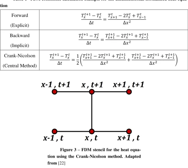
3 In the FDM, the coefficients used can be calculated using an: explicit, implicit or mixed

(Also known as Crank-Nicolson) method/scheme. This means that if the approximations are made

using forward, backward or central approach, they vary in accuracy and amount of calculation required from smaller to greater, respectively. Table 1 shows the FDM discretization of Eq. (1)

Figure 3 shows the FDM node stencil for the unidimensional normalized heat equation.

𝜕𝑇 𝜕𝑡 =

𝜕2_𝑇

𝜕𝑥2 (1)

Table 1 –FDM coefficient calculation example for the unidimensional normalized heat

equa-tion

Forward

(Explicit)

𝑇𝑥𝑡+1− 𝑇𝑥𝑡

∆𝑡 =

𝑇𝑥+1𝑡 − 2𝑇𝑥𝑡+ 𝑇𝑥−1𝑡

∆𝑥2

Backward

(Implicit)

∆𝑡 =

𝑇𝑥+1𝑡+1− 2𝑇𝑥𝑡+1+ 𝑇𝑥−1𝑡+1

∆𝑥2

Crank-Nicolson

(Central Method)

∆𝑡 =

1 2 (

𝑇𝑥+1𝑡+1− 2𝑇𝑥𝑡+1+ 𝑇𝑥−1𝑡+1

∆𝑥2 +

𝑇𝑥+1𝑡+1− 2𝑇𝑥𝑡+1+ 𝑇𝑥−1𝑡+1

∆𝑥2 )

The problems associated with this type of modeling have been studied for the RCC, it is the LCC that requires attention and the main difference is symmetry, for RCC we can simplify

our problem by considering a unidimensional or bi-dimensional problem. Only in the latter case

can we start to see transverse segregation but most articles consider only the first case. With LCC we must consider a tri-dimensional problem, not only increasing in complexity but also in sheer

data volume. Velhinho et al. [9], [10] stated the problems related to this modeling and Gonçalo

et al. [11] studied transverse segregation. From these studies resulted that there are three types of segregation to study: reverse, dimensional and transverse segregation.

Figure 3 – FDM stencil for the heat

equa-tion using the Crank-Nicolson method. Adapted

(26)

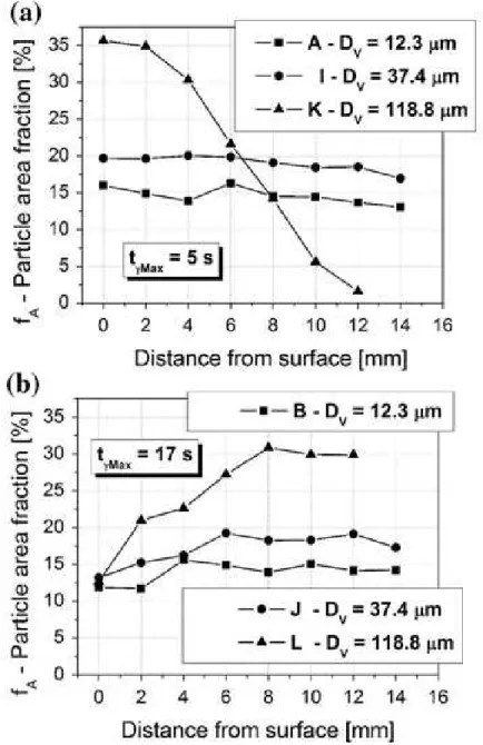
Figure 4 – Particle area fraction profile for FGMMC cast by

LCC of Al/SiC. a) Spin-up time of 5s; b) Spin-up time of 17s. Dv is the

mean particle size; A, I, K, B, J, L were experiments made; 0 is the

furthest point from the centrifugal axis. Adapted from [9]

1.3 Reverse Segregation:

(27)

5

1.4 Dimensional Segregation:

As with reverse segregation, we observe that instead of larger particles occupying

posi-tions near the surface, smaller particles that take this position (Figure 5 b)). Centrifugal

accelera-tion is higher for larger particles; it was expected

that the opposite would happen. The effect hap-pens due to the solidification front; the dendritic

growth of Al crystals during solidification blocks

larger particles more easily than smaller ones,

and in some cases, allows smaller particles to travel further towards the surface.

1.5 Transverse segregation

The final problem not considered in RCC is transverse segregation. Transverse segregation

is the effect of particle variation along the axis perpendicular to its movement. This occurs

be-cause the solidification front is faster around the surface then in the parts core, causing particles to stop earlier than the ones closer to the center, therefore causing a transverse gradient; particle

pushing also helps in the formation of such gradient but not as strongly. [9]–[11]

1.6 Synthesis

We now have all the necessary information to simulate the production of an Al/SiC FGMMC produced by LCC using a three-dimensional mesh. This type of mesh isn’t commonly

used in calculations, as problems tend to be simplified towards bi-dimensional or unidimensional

solutions. In the next chapters, we will explain the nuances related to the application of FDM, namely: equation solving order, parameters used and assumptions made. Latter we explain in

detail how each equation is solved, before presenting and analyzing some simulation results for

particular cases of interest.

Figure 6 – Transverse segregation. Adapted from [9]

Figure 5 – Mean particle diameter

(28)

(29)

7 Figure 7 – Particle Movement. Adapted from [16]

2 Numerical Model

In this section, how the computer model works, all the equations used and iterative method

are explained.

2.1 Initialization

At the beginning of each time step we take the values of particle fraction (FP), solid fraction (FS) and temperature from the previous time step (initial conditions for the first time step) and

use them for this step. On each subsequent iteration, we use the FS obtained in the previous

iter-ation and feed it until convergence is achieved. Liquid fraction (FL) is obtained at each iteriter-ation using both the FP and FS.

2.2 Particle Movement

At each time step, we calculate the apparent particle velocity based on the equations of Gao et al. [15], this equation was derived from Stoke’s equation for particle motion:

𝒗𝒑 =(𝜌𝑃− 𝜌𝐿)𝜀𝑃𝜔

2_𝑅𝑑2_{(1 − 𝜀} 𝑃)4,65

18𝜇𝑙(1 − 𝜀𝐿)(𝜀𝑃+ 𝜀𝐿)2

(2)

Where angular velocity 𝜔 is:

𝜔 =2𝜋 ∗ 𝑟𝑝𝑚₆₀ (3)

At this point, maximum particle clustering and the solidification front are not considered.

(30)

is given by the number of particles in that time step, minus the particles leaving plus the particle

entering:

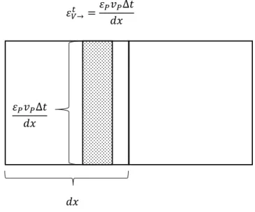
𝜀𝑗𝑘𝑙𝑡+1= 𝜀𝑗𝑘𝑙𝑡 − 𝜀𝑉→𝑡 + 𝜀→𝑉𝑡 (4) The amount of particle leaving a control volume is the same entering the control volume

next to it. The particle displacement can be determined by multiplying the velocity by the time

step and dividing it by the cell size in the x component. If we multiply that by the number of particles in that volume, we get the particle fraction that exits that volume:

𝜀𝑉→𝑡 =𝜀𝑃_𝑑𝑥𝑣𝑃∆𝑡 (5)

The particle clustering is limited to 52%, value given by Watanabe et al. [17], value ob-tained for the Al/SiC system. We also assume the particles stop upon reaching the solidification

front. A consequence of this method though is that particles can only move from one cell to the

next, following this rule:

𝑣𝑃∆𝑡 < 𝑑𝑥 (6)

This means that:

∆𝑡 <𝑑𝑥_𝑣

𝑃

(7)

Liquid fraction are now calculated using the constitutive equation:

𝜀𝑆+ 𝜀𝐿+ 𝜀𝑃= 1 (8)

For the next time step we will need all the previous calculations to the best of detail. This means that the particle velocity equation used before isn’t accurate enough, but we know the actual particle movement so we can simply calculate the actual particle movement by comparing

the previous particle fraction vector with the current one

𝑑𝑥 𝜀𝑃𝑣𝑃∆𝑡

𝑑𝑥

(31)

9

2.3 Temperature Field

We now have all the basis used to update the temperature field. For that we use the heat

equation given by Rappaz et. al. [18]:

𝜕

𝜕𝑡(𝜌𝐻) + 𝑑𝑖𝑣(𝜌𝐻𝑣) + 𝑑𝑖𝑣(𝑗𝑇) = 𝑄̇𝑇 (9)

In which the first term 𝜕

𝜕𝑡(𝜌𝐻) is associated with the energy stored in the material, the

second term 𝑑𝑖𝑣(𝜌𝐻𝑣) with the energy present in moving phases (particle and liquid), the third

term 𝑑𝑖𝑣(𝑗_𝑇) is the Fourier’sLaw for a diffusive heat flux and the last is the energy transferred into or out of the system.

The last term 𝑄̇_𝑇, related to heat supplied or taken from the system by inside agents is considered zero for the purposes of finding the thermal equilibrium.

The latent heat of fusion L is only considered when calculating solidification.

The rest of the equation results in the following (note that particle movement is only

con-sidered along the x-axis):

𝜕

𝜕𝑡 [(𝜌𝑠𝜀𝑠𝐶𝑃𝑠+ 𝜌𝑃𝜀𝑝𝐶𝑃𝑃+ 𝜌𝐿𝜀𝐿𝐶𝑃𝐿)𝑇] + 𝜕

𝜕𝑥[(𝜌𝑃𝜀𝑃𝐶𝑃𝑃𝒗𝑃+ 𝜌𝐿𝜀𝐿𝐶𝑃𝐿𝒗𝐿)𝑇] = 𝜕

𝜕𝑥 [(𝜀𝑆𝐾𝑆+ 𝜀𝑃𝐾𝑃+ 𝜀𝐿𝐾𝐿) 𝜕𝑇 𝜕𝑥] +

𝜕

𝜕𝑦 [(𝜀𝑆𝐾𝑆+ 𝜀𝑃𝐾𝑃+ 𝜀𝐿𝐾𝐿) 𝜕𝑇 𝜕𝑦] + 𝜕

𝜕𝑧 [(𝜀𝑆𝐾𝑆+ 𝜀𝑃𝐾𝑃+ 𝜀𝐿𝐾𝐿) 𝜕𝑇 𝜕𝑧]

(10)

We solve the equation in order of 𝑇 using a central difference scheme for the FDM

coeffi-cients and arrive at an equation of the following form:

𝑇𝑡 _{= 𝑇}𝑡+1_{𝐽 + 𝑇}

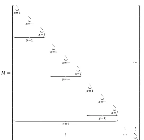
𝑗+1𝑡+1𝐽++ 𝑇𝑗−1𝑡+1𝐽−+ 𝑇𝑘+1𝑡+1𝐾++ 𝑇𝑘−1𝑡+1𝐾−+ 𝑇𝑙+1𝑡+1𝐿++ 𝑇𝑙−1𝑡+1𝐿− (11) For simplicity and time saving we assume a Dirichlet Boundary Condition of 𝑇 = 𝑇_𝑒, 𝑇_𝑒 being the mold temperature. We arrange the coefficients in the matrix and multiply it by the

cur-rent temperature field:

𝑇𝑡+1_{= 𝑀\𝑇}𝑡 ₍₁₂₎

In which T is a vector of size 𝑥 ∗ 𝑦 ∗ 𝑧 and M is a sparse square matrix of dimension

(32)

𝑀 = [ ⋱⏟_𝑥=1 ⋱⏟ 𝑥=⋯ ⋱⏟ 𝑥=𝑗 ⏟ 𝑦=1 ⋱⏟ 𝑥=1 ⋱⏟ 𝑥=⋯ ⋱⏟ 𝑥=𝑗 ⏟ 𝑦=⋯ ⋱⏟ 𝑥=1 ⋱⏟ 𝑥=⋯ ⋱⏟ 𝑥=𝑗 ⏟ 𝑦=𝑘 ⏟ 𝑧=1 ⋯ ⋱ ⋮ ⋮ ⋯ ⋱⏟ 𝑧=𝑙]

For a given 𝑗𝑘𝑙 coordinate, we determine the corresponding row:

𝑆 = 𝑗 + (𝑘 − 1)𝑥 + (𝑙 − 1)𝑥𝑦 (13)

In this row, we organize the constants’ information per the following table:

Table 2 –Coefficients’ position.

Coefficient Row

𝐽 𝑆

𝐽+ 𝑆 + 1

𝐽− 𝑆 − 1

𝐾+ 𝑆 + 𝑥

𝐾− 𝑆 − 𝑥

𝐿+ 𝑆 + 𝑥𝑦

𝐿− 𝑆 − 𝑥𝑦

For a 3 ∗ 3 ∗ 3 system, the result would be a 27 by 27 sparse matrix where the only position

(33)

11

[

⋱ …⏟

𝑦=1

… 𝐿− …

⏟ 𝑦=2 …⏟ 𝑦=2 ⏟ 𝑧=1

… 𝐾− …

⏟

𝑦=1

𝐽− 𝐽 𝐽+

⏟

𝑦=2

… 𝐾+ …

⏟ 𝑦=2 ⏟ 𝑧=2 …⏟ 𝑦=1

… 𝐿+ …

⏟ 𝑦=2 …⏟ 𝑦=2 ⏟ 𝑧=3 ⋱ ]

2.4 Enthalpy Field

After estimating the temperature update, we determine the correspondent enthalpy field using the following relation:

𝐻𝑡+1_{= 𝐻}𝑡_{− ∫} _〈𝜌𝐶 𝑃〉 𝑇𝑡+1

𝑇𝑡 𝑑𝑇

(14)

In which 〈𝜌𝐶_𝑃〉 can be seen has average properties in each node 𝜌_𝑠𝜀_𝑠𝐶_𝑃𝑠+ 𝜌_𝑃𝜀_𝑝𝐶_𝑃𝑃+

𝜌𝐿𝜀𝐿𝐶𝑃𝐿, simplified gives us:

𝐻𝑡+1_{= 𝐻}𝑡_{− 〈𝜌𝐶}

𝑃〉(𝑇𝑡+1− 𝑇𝑡) (15)

This gives us an approximated enthalpy field used to determine the solid update.

2.5 Solidification

There are many methods to simulate a solidification front. They range from front-tracking,

source-term and enthalpy formulations. In this work a variation of the latter example is used, the temperature recovery method (TRM); first devised by Tszeng [19].

In the TRM the solidification process used in FDM schemes and FEM, it’s formulated based on the temperature and enthalpy fields and is

very easy to apply. The first step is to calculate

the thermal equilibrium for a given time step us-ing the previous equations, usus-ing the relation

be-tween temperature and enthalpy [20]:

𝐻(𝑇) = ∫ 𝜌𝐶𝑝𝑑𝑇 𝑇 𝑇𝑟

+ 𝜌𝐿 (16)

Assuming the reference temperature (𝑇_𝑟) is the alloy’s melting point (𝑇𝑚), with each time

step we obtain a ∆T, feeding this into equation (15) we can determine the ∆H that occurred,

do-ing this we can obtain the enthalpy field, furthermore, if we divide the enthalpy variation by the

latent heat we obtain the liquid fraction that solidified in this time step (Figure 9).

Figure 9 – Enthalpy in function of

(34)

2.6 Convergence

Properties vary with difference fractions, as such convergence is necessary. At this step,

we save the current solid fraction and iterate the time step again with the updated solid fraction, this step is repeated until the difference between this iterations’ enthalpy field minus the previous iterations’ is under a certain tolerance, normally 𝑇𝑂𝐿 < 10−5

2.7 Iteration

After convergence in the enthalpy field is achieved, a new time step is calculated using the

(35)

13

3 Method

The simulations were made using MATLAB version R2016b in a 64-bit Windows 10

Ed-ucation operative system with 12,0 GB of RAM and an Intel® Xeon® CPU E5506 @ 2.13GHz

2.13 GHz processor.

In the procedure developed in the present work, the equations were solved iteratively using

a fixed-grid, single-domain FDM. The advection equations were discretized using an explicit

scheme while an implicit one was used for the heat equation, the coefficients used are calculated using a central scheme. For the solidification, an enthalpy method was used. The equations were

solved iteratively in the following manner:

1. Import values from the previous time step

2. Determine particle velocity from Eq. (2)

3. Calculate particle displacement from Eq. (5)

4. Obtain new liquid phase from Eq. (8)

5. Compute the new temperature field T from Eq. (9)

6. Determine the enthalpy field from Eq. (15)

7. Guess solidification using Eq. (16)

8. Iterate until convergence in the enthalpy field

This general procedure was used during each time step. The exception was the first time

where the starting values were used. All the simulations were using dimensions of 8 ∗ 4 ∗ 4 cm,

1000 rpm and a TOL of 10−5.

Despite many attempts, an implicit method for the advection equation wasn’t possible to implement, and an explicit method was used instead. The decision to maintain an implicit scheme for the heat equation instead of an explicit one comes from the coefficient restriction of the

ex-plicit method. Unlike the imex-plicit method, which is always numerically stable and convergent,

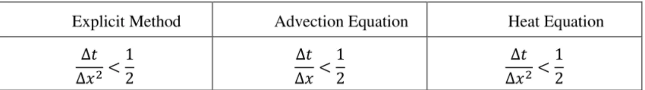
the numeric stability and convergence of the explicit method require that the conditions in Table 3 be attained [13]:

Table 3 – Explicit method convergence

Explicit Method Advection Equation Heat Equation

∆𝑡 ∆𝑥2<

1 2 ∆𝑡 ∆𝑥 < 1 2 ∆𝑡 ∆𝑥2 <

1 2

(36)

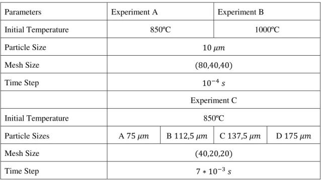
Table 4 – Different parameters used

Parameters Experiment A Experiment B

Initial Temperature 850ºC 1000ºC

Particle Size 10 𝜇𝑚

Mesh Size (80,40,40)

Time Step 10−4 𝑠

Experiment C

Initial Temperature 850ºC

Particle Sizes A 75 𝜇𝑚 B 112,5 𝜇𝑚 C 137,5 𝜇𝑚 D 175 𝜇𝑚

Mesh Size (40,20,20)

Time Step 7 ∗ 10−3 𝑠

The constants used were:

Table 5 – Properties of Al/SiC. Adapted from [14]

Quantity Symbol Value Units

Liquid Density (Al) 𝜌_𝐿 2390 𝑘𝑔/𝑚3

Solid Density (Al) 𝜌_𝑆 2550 𝑘𝑔/𝑚3

Particle Density (SiC) 𝜌_𝑃 3200 𝑘𝑔/𝑚3

Liquid Specific Heat (Al) 𝐶_𝑃𝐿 1079.5 𝐽/𝑘𝑔 𝐾

Solid Specific Heat (Al) 𝐶_𝑃𝑆 1176.5 𝐽/𝑘𝑔 𝐾

Particle Specific Heat (SiC) 𝐶_𝑃𝑃 840 𝐽/𝑘𝑔 𝐾

Liquid Thermal Conductivity (Al) 𝐾_𝐿 95 𝑊/𝑚𝐾

Solid Thermal Conductivity (Al) 𝐾_𝑆 210 𝑊/𝑚𝐾

Particle Thermal Conductivity (SiC) 𝐾_𝑃 16 𝑊/𝑚𝐾

Latent Heat of Fusion (pure Al) 𝐿 _{3.97 ∗ 10}5 𝐽/𝑘𝑔

Melting Temperature (pure Al) 𝑇_𝑚 933.6 𝐾

Mold Temperature 𝑇_𝑒 300 𝐾

(37)

15

3.1 Assumptions

The equations were formulated and solved per the following assumptions:

 Heat transfer occurs strictly due to conduction

 No energy loss due to radiation or convection

 Thermal equilibrium inside each control volume is reached instantly

 Gravity is neglected

 Solidification front is considered planar

 Angular velocity is constant and is achieved instantly

 Particles reach terminal velocity instantly

 There is no particle pushing by the solidification front

 Particles stop the instant they reach the solidification front

 Particles are non-deformable, spherical and chemically inert

 Initial particle positions are considered uniform across the melt

 There is no change in volume

 Thermophysical properties are considered constant

(38)

(39)

17

4 Results and Discussion

4.1 Results

Three experiments (Table 4) were made using the above methods. The first two were made

using a fine mesh and small time step, resulting in a high-quality surface used to compare two different initial temperatures. The final experiment was ran using four particle sizes at the same

time to simulate granulometry, this was made in a lower resolution.3.2.1 Main Experiments

In the first result clearly observe the effect of transverse segregation.

Figure 10 – Percentage surface for particles along the 20mm height. This is a result of

(40)

In the side-view we can see the phenomenon of severse segregation, even without considering particle pushing. This is a good indicator that particle pushing contributes only

slightly to this effect.

Similarly to experiment A we can observe the effect of transverse segregation, we can’t compare these two figures but both show prominent results.

Figure 12 – Side-view of percentage surface for particles along the 20mm height. This is a

result of experiment A

(41)

19 Comparing both results we can see the effects of different starting condittions, namely, we

can observe that for higher starting temperatures the particle distribution peaks closer to the surface, another note is that the particles peak higher than for lower temperatures.

(42)

4.2 Effects of reinforcement particle size distribution

We can observe the effect of transverse segregation, even if lessened by the bigger particle

sizes. The plateau observed is stuck at 52% because that was the theoretical limit set [17].

We can observe a minor case of reverse segregation, this effect is dulled due to the particle

sizes used, the larger they are, smaller the result.

Figure 15 – Side-view of percentage surface for particles along the 20mm height. This result is

of experiment C.

(43)

21 We can see that bigger particles arrive near the surface faster, occupying space and not

letting other particle in there; we can also see that from the smaller to the bigger particles the profiles change showing this effect.

(44)

(45)

23

5 Conclusions and Future Work

5.1 Conclusions

A MATLAB code has been developed, capable of simulating the production of any LCC

FGMMC. The code is robust, precise and it can simulate a panoply of different starting condi-tions; however, its main downside concerns the execution time to perform detailed calculations.

As such, a low-resolution simulation is advised as a way to predict any problems or the expect

time of completion for a high-resolution simulation.

Despite not taking particle pushing into account, we can clearly observe the effect of

re-verse segregation, either when particle grain size is considered to be homogeneous or when

vari-ations of this parameter are taken into account. This shows us that particle impediment is an im-portant contributor for this effect.

We can also see that for a higher starting temperature particles reach further and a higher

concentration is obtained. With the model currently operational we can easily study this.

In the simulated results, we can observe that larger particles reach the surface faster than

smaller ones, this is expected as larger particles have a higher velocity. What happens in

experi-mental results is that smaller particles reach further than larger one. This means that the effects of particle pushing and non-planar solidification are responsible and critical for the effect of

di-mensional segregation.

The effect of transverse segregation is clearly visible, which goes according with previous works [10].

5.2 Future Work

For the future, there are two main areas of development: model improvement and speed.

For the model improvement:

 Migrating to a Finite Element Method might be advantageous for complex ge-ometries and commercial applications.

 Using a Neumann boundary condition is more accurate but requires extra calcu-lation time.

 Considering a non-planar solidification front might reveal more insight and flexi-bility to the process.

For speed:

(46)

 The complete change to either implicit or explicit method, depending on the so-lidification time. The first method is better for transient and timely casts while the second one is better for fast changing processes.

Notes:

(47)

25

5 Bibliography

[1] R. M. Mahamood, E. T. A. Member, M. Shukla, and S. Pityana, “Functionally Graded Material : An Overview,” World Congr. Eng., vol. III, pp. 2–6, 2012.

[2] T. P. D. Rajan and B. C. Pai, “Developments in Processing of Functionally Gradient Metals and Metal–Ceramic Composites: A Review,” Acta Metall. Sin. (English Lett., vol. 27, no. 5, pp. 825–838, 2014.

[3] A. Gupta and M. Talha, “Recent development in modeling and analysis of functionally graded materials and structures,” Prog. Aerosp. Sci., vol. 79, pp. 1–14, 2015.

[4] A. Bahrami, M. I. Pech-Canul, C. A. Gutierrez, and N. Soltani, “Effect of rice-husk ash on properties of laminated and functionally graded Al/SiC composites by one-step pressureless infiltration,” J. Alloys Compd., vol. 644, pp. 256–266, 2015.

[5] M. Pourmajidian and F. Akhlaghi, “Fabrication and Characterization of Functionally Graded Al/SiCp Composites Produced by Remelting and Sedimentation Process,” J. Mater. Eng. Perform., vol. 23, no. 2, pp. 444–450, 2014.

[6] T. P. D. Rajan, E. Jayakumar, and B. C. Pai, “Developments in solidification processing of functionally graded aluminium alloys and composites by centrifugal casting technique,” Trans. Indian Inst. Met., vol. 65, no. 6, pp. 531–537, 2012.

[7] H. Pointner, A. De Gracia, J. Vogel, N. H. S. Tay, M. Liu, M. Johnson, and L. F. Cabeza, “Computational efficiency in numerical modeling of high temperature latent heat storage : Comparison of selected software tools based on experimental data,” Appl. Energy, vol. 161, pp. 337–348, 2016.

[8] C. Grossmann, H. Roos, and M. (Martin. Stynes, “Numerical Treatment of Partial Differential Equations,” 2007.

[9] A. Velhinho and L. A. Rocha, “Longitudinal centrifugal casting of metal-matrix functionally graded composites : an assessment of modelling issues,” J. Mater. Sci., vol. 46, no. 11, pp. 3753–3765, 2011.

[10] A. Velhinho, G. Rodrigues, J. P. Mota, and R. Martins, “Modelling of transverse segregation on centrifugally-cast functionally graded composites,” pp. 1–8, 2014.

[11] G. da C. Rodrigues, “Lisboa08/2011,” Universidade Nova de Lisboa, 2011.

[12] X.-H. Chen and H. Yan, “Solid–liquid interface dynamics during solidification of Al 7075–Al2O3np based metal matrix composites,” Mater. Des., vol. 94, pp. 148–158, 2016.

[13] J. Crank, “THE MATHEMATICS OF DIFFUSION,” 1975.

[14] J. W. Gao and C. Y. Wang, “Modeling the solidification of functionally graded materials by centrifugal casting,” Mater. Sci. Eng. A, vol. 292, no. 2, pp. 207–215, 2000.

[15] J. W. Gao and C. Y. Wang, “Transport Phenomena During Solidification Processing of Functionally Graded Composites by Sedimentation,” J. Heat Transfer, vol. 123, no. 2, p. 368, 2001.

(48)

[17] Y. Watanabe, N. Yamanaka, and Y. Fukui, “Control of composition gradient in a metal -ceramic functionally graded material manufactured by the centrifugal method,” Compos. Part A Appl. Sci. Manuf., vol. 29, no. 5–6, pp. 595–601, 1998.

[18] M. Rappaz, M. Bellet, and M. Deville, Numerical Modeling in Materials Science and Engineering, vol. 32. 2003.

[19] T. C. Tszeng, Y. T. Im, and S. Kobayashi, “Thermal analysis of solidification by the temperature recovery method,” Int. J. Mach. Tools Manuf., vol. 29, no. 1, pp. 107–120, 1989.

[20] V. R. Voller and C. R. Swaminathan, “FIXED GRID TECHNIQUES FOR PHASE CHANGE PROBLEMS : A REVIEW,” vol. 30, pp. 875–898, 1990.

[21] E. M. Agaliotis, M. R. Rosenberger, a. E. Ares, and C. E. Schvezov, “Influence of the Shape of the Particles in the Solidification of Composite Materials,” Procedia Mater. Sci., vol. 1, pp. 58–63, 2012.

[22] G. Biswas, “Finite difference method,” vol. 6, no. 10. p. 9685, 2011.

(49)

27

Appendix 1: Heat Equation Deduction

Constituent Equation:

𝜀𝑆+ 𝜀𝐿+ 𝜀𝑃= 1 (17)

Average thermal conductivity:

〈𝐾〉 = 𝜀𝑆𝐾𝑆+ 𝜀𝑃𝐾𝑃+ 𝜀𝐿𝐾𝐿 (18) Average volumetric specific heat:

〈𝜌𝐶𝑝〉 = 𝜌𝑠𝜀𝑠𝐶𝑃𝑠+ 𝜌𝑃𝜀𝑝𝐶𝑃𝑃+ 𝜌𝐿𝜀𝐿𝐶𝑃𝐿 (19) The heat equation used at each time step is given by Rappaz et. al. [1]:

𝜕

𝜕𝑡(𝜌𝐻) + 𝑑𝑖𝑣(𝜌𝐻𝑣) + 𝑑𝑖𝑣(𝑗𝑇) = 𝑄̇𝑇 (9)

Extending all terms:

𝜕

𝜕𝑡 [(𝜌𝑠𝜀𝑠𝐶𝑃𝑠+ 𝜌𝑃𝜀𝑝𝐶𝑃𝑃+ 𝜌𝐿𝜀𝐿𝐶𝑃𝐿)𝑇] + 𝜕

𝜕𝑥[(𝜌𝑃𝜀𝑃𝐶𝑃𝑃𝒗𝑃+ 𝜌𝐿𝜀𝐿𝐶𝑃𝐿𝒗𝐿)𝑇] =_{𝜕𝑥 [}𝜕 (𝜀𝑆𝐾𝑆+ 𝜀𝑃𝐾𝑃+ 𝜀𝐿𝐾𝐿)_{𝜕𝑥] +}𝜕𝑇 _{𝜕𝑦 [}𝜕 (𝜀𝑆𝐾𝑆+ 𝜀𝑃𝐾𝑃+ 𝜀𝐿𝐾𝐿)𝜕𝑇_𝜕𝑦]

+_{𝜕𝑧 [}𝜕 (𝜀𝑆𝐾𝑆+ 𝜀𝑃𝐾𝑃+ 𝜀𝐿𝐾𝐿)𝜕𝑇_𝜕𝑧]

(10)

Using the substitution [2]:

𝒗𝐿= −𝜀𝑃_𝜀𝒗𝑃

𝐿 (20)

We arrive at:

(𝜕𝜀_{𝜕𝑡 𝜌}𝑠 𝑠𝐶𝑃𝑠+𝜕𝜀_{𝜕𝑡 𝜌}𝑝 𝑃𝐶𝑃𝑃+𝜕𝜀_{𝜕𝑡 𝜌}𝐿 𝐿𝐶𝑃𝐿)

⏟

𝐴

𝑇 + (𝜌⏟ 𝑠𝜀𝑠𝐶𝑃𝑠+ 𝜌𝑃𝜀𝑝𝐶𝑃𝑃+ 𝜌𝐿𝜀𝐿𝐶𝑃𝐿) 𝐵

𝜕𝑇 𝜕𝑡

+_{𝜕𝑥 [}𝜕 (𝜌⏟ 𝑃𝐶𝑃𝑃− 𝜌𝐿𝐶𝑃𝐿) 𝐶

𝜀𝑃𝒗𝑃𝑇]

+ (_⏟𝜕𝜀_{𝜕𝑥 𝐾}𝑆 𝑆+𝜕𝜀_{𝜕𝑥 𝐾}𝑃 𝑃+𝜕𝜀_{𝜕𝑥 𝐾}𝐿 𝐿) 𝐷𝑥

𝜕𝑇

𝜕𝑥 +(𝜀⏟ 𝑆𝐾𝑆+ 𝜀𝑃_𝐸𝐾𝑃+ 𝜀𝐿𝐾𝐿) 𝜕2_𝑇

𝜕𝑥2

+ (_⏟𝜕𝜀_{𝜕𝑦 𝐾}𝑆 𝑆+𝜕𝜀_{𝜕𝑦 𝐾}𝑃 𝑃+𝜕𝜀_{𝜕𝑦 𝐾}𝐿 𝐿) 𝐷𝑦

𝜕𝑇

𝜕𝑦 +(𝜀⏟ 𝑆𝐾𝑆+ 𝜀𝑃_𝐸𝐾𝑃+ 𝜀𝐿𝐾𝐿) 𝜕2_𝑇

𝜕𝑦2

(50)

+ (𝜕𝜀𝑆 𝜕𝑧 𝐾𝑆+

𝜕𝜀𝑃

𝜕𝑧 𝐾𝑃+ 𝜕𝜀𝐿

𝜕𝑧 𝐾𝐿) ⏟

𝐷𝑧

𝜕𝑇

𝜕𝑧 +(𝜀⏟ 𝑆𝐾𝑆+ 𝜀𝑃_𝐸𝐾𝑃+ 𝜀𝐿𝐾𝐿) 𝜕2_𝑇

𝜕𝑧2

We use the letter substitutions to simplify writing and arrive at:

𝐴𝑇 + 𝐵𝜕𝑇 𝜕𝑡 + 𝐶

𝜕𝜀𝑃

𝜕𝑥 𝑣𝑃 ⏟

𝐹1

𝑇 + 𝐶𝜕𝑣𝑃 𝜕𝑥 𝜀𝑃 ⏟

𝐹2

𝑇 +𝜕𝑇 𝜕𝑥 𝜀⏟ 𝑃𝑣_𝐹𝑃𝐶

3

= 𝐷𝑥𝜕𝑇_{𝜕𝑥 + 𝐷}𝑦𝜕𝑇_{𝜕𝑦 + 𝐷}𝑧𝜕𝑇_{𝜕𝑧 + 𝐸 (}𝜕 2_𝑇

𝜕𝑥2+

𝜕2_𝑇

𝜕𝑦2+

𝜕2_𝑇

𝜕𝑧2)

(22)

(=)

𝑇(𝐴 + 𝐹1+ 𝐹2) + 𝐵𝜕𝑇_{𝜕𝑡 + 𝐹}3𝜕𝑇_𝜕𝑥

= 𝐷𝑥𝜕𝑇_{𝜕𝑥 + 𝐷}𝑦𝜕𝑇_{𝜕𝑦 + 𝐷}𝑧𝜕𝑇_{𝜕𝑧 + 𝐸 (}𝜕 2_𝑇

𝜕𝑥2+

𝜕2_𝑇

𝜕𝑦2+

𝜕2_𝑇

𝜕𝑧2)

(23)

Unfolding 𝜕𝑇

𝜕𝑡 using the FDM:

𝑇𝑡+1_{− 𝑇}𝑡

∆𝑡 𝐵 = ⋯ (24)

And evaluating all other terms at time 𝑡 + 1:

𝑇𝑡 _{= 𝑇}𝑡+1_{[1 +}∆𝑡

𝐵 (𝐴 + 𝐹1+ 𝐹2)] ⏟

𝐺

+ (_⏟𝐹3_{𝐵 −}∆𝑡 𝐷𝑥_{𝐵 )}∆𝑡

𝐻𝑥

𝜕𝑇 𝜕𝑥

−𝐷𝑦_𝐵∆𝑡 ⏟

𝐻𝑦

𝜕𝑇 𝜕𝑦 −

𝐷𝑧∆𝑡

𝐵 ⏟ 𝐻𝑧 𝜕𝑇 𝜕𝑧 − 𝐸∆𝑡 𝐵 ⏟ 𝐼

(_𝜕𝑥𝜕2𝑇₂+_𝜕𝑦𝜕2𝑇₂+𝜕_𝜕𝑧2𝑇₂)

(25)

(=)

𝑇𝑡 _{= 𝑇}𝑡+1_{𝐺 + 𝐻} 𝑥𝑇𝑗+1

𝑡+1_{− 𝑇} 𝑗−1𝑡+1

2∆𝑥 + 𝐻𝑦

𝑇𝑘+1𝑡+1− 𝑇𝑘−1𝑡+1

2∆𝑦 + 𝐻𝑧

𝑇𝑙+1𝑡+1− 𝑇𝑙−1𝑡+1

2∆𝑧

−𝐼 (𝑇𝑗+1𝑡+1− 2𝑇_∆𝑥𝑗𝑡+1₂ + 𝑇𝑗−1𝑡+1+𝑇𝑘+1𝑡+1− 2𝑇_∆𝑦𝑘𝑡+1₂ + 𝑇𝑘−1𝑡+1+𝑇𝑙+1𝑡+1− 2𝑇_∆𝑧𝑙𝑡+1₂ + 𝑇𝑙−1𝑡+1)

(26)

(=)

𝑇𝑡 _{= 𝑇}𝑡+1_{[𝐺 − 𝐼 (} 1

∆𝑥2+

1 ∆𝑦2+

1 ∆𝑧2)]

⏟

𝐽

+𝑇𝑗+1𝑡+1(_⏟_{2∆𝑥 −}𝐻𝑥 _∆𝑥𝐼2) 𝐽+

+ 𝑇𝑗−1𝑡+1(−_⏟_{2∆𝑥 −}𝐻𝑥 _∆𝑥𝐼2) 𝐽−

+ 𝑇𝑘+1𝑡+1(_⏟_{2∆𝑦 −}𝐻𝑦 _∆𝑦𝐼2) 𝐾+

(51)

29

+𝑇_𝑘−1𝑡+1₍₋ 𝐻𝑦

2∆𝑦 − 𝐼 ∆𝑦2)

⏟

𝐾−

+ 𝑇_𝑙+1𝑡+1₍𝐻𝑧

2∆𝑧 − 𝐼 ∆𝑧2)

⏟

𝐿+

+ 𝑇_𝑙−1𝑡+1₍₋ 𝐻𝑧

2∆𝑧 − 𝐼 ∆𝑧2)

⏟

𝐿−

We now arrive at an equation of the form:

𝑇𝑡 _{= 𝑇}𝑡+1_{𝐽 + 𝑇}

𝑗+1𝑡+1𝐽++ 𝑇𝑗−1𝑡+1𝐽−+ 𝑇𝑘+1𝑡+1𝐾++ 𝑇𝑘−1𝑡+1𝐾−+ 𝑇𝑙+1𝑡+1𝐿++ 𝑇𝑙−1𝑡+1𝐿− (11) Of which:

𝐽 = 1 +∆𝑡(𝜌𝑃𝐶_〈𝜌𝐶𝑃𝑃− 𝜌𝐿𝐶𝑃𝐿)

𝑝〉 (

𝜕𝜀𝑃

𝜕𝑥 𝑣𝑃+ 𝜕𝑣𝑃

𝜕𝑥 𝜀𝑃) +

𝜕〈𝜌𝐶𝑝〉

𝜕𝑡 ∆𝑡 〈𝜌𝐶𝑝〉

+2∆𝑡〈𝐾〉_〈𝜌𝐶

𝑝〉 (

1 ∆𝑥2+

1 ∆𝑦2+

1 ∆𝑧2)

(28)

𝐽+=∆𝑡𝜀𝑃𝒗𝑃_{2∆𝑥〈𝜌𝐶}(𝜌𝑃𝐶𝑃𝑃− 𝜌𝐿𝐶𝑃𝐿)

𝑝〉 −

𝜕〈𝐾〉 𝜕𝑥

∆𝑡 2∆𝑥〈𝜌𝐶𝑝〉 −

∆𝑡〈𝐾〉 〈𝜌𝐶𝑝〉∆𝑥2

(29)

𝐽−= −∆𝑡𝜀𝑃𝒗𝑃_{2∆𝑥〈𝜌𝐶}(𝜌𝑃𝐶𝑃𝑃− 𝜌𝐿𝐶𝑃𝐿)

𝑝〉 +

𝜕〈𝐾〉 𝜕𝑥

∆𝑡 2∆𝑥〈𝜌𝐶𝑝〉 −

∆𝑡〈𝐾〉

〈𝜌𝐶𝑝〉∆𝑥2 (30)

𝐾+= −𝜕〈𝐾〉_𝜕𝑦 _{2∆𝑦〈𝜌𝐶}∆𝑡 𝑝〉 −

∆𝑡〈𝐾〉

〈𝜌𝐶𝑝〉∆𝑦2 (31)

𝐾−=𝜕〈𝐾〉_𝜕𝑦 _{2∆𝑦〈𝜌𝐶}∆𝑡 𝑝〉 −

∆𝑡〈𝐾〉

〈𝜌𝐶𝑝〉∆𝑦2 (32)

𝐿+= −𝜕〈𝐾〉_𝜕𝑧 _{2∆𝑧〈𝜌𝐶}∆𝑡 𝑝〉 −

∆𝑡〈𝐾〉

〈𝜌𝐶𝑝〉∆𝑧2 (33)

𝐿−=𝜕〈𝐾〉_𝜕𝑧 _{2∆𝑧〈𝜌𝐶}∆𝑡 𝑝〉 −

∆𝑡〈𝐾〉

(52)

(53)

31

Appendix 2: Main Function Code

function [ VP,FP,FL,FS,T2imp] = Simulate(

x,re,ri,y,Y,z,Z,t,passo,FRi,Ti,Te,rpmi,sut,TOL)

% Test Function

%

[VP,FP,FL,FS,T2imp]=Simu-

late(20,0.38,0.3,10,0.04,10,0.04,90,0.5,0.1,1120,300,1000,5,120*10e-6);

%

% Entry:

% "x" % Matrix dimension in x

% "re" % Exterior radius in m

% "ri" % Interior radius in m

% "y" % Matrix dimension in y

% "Y" % Dimension Y in m

% "z" % Matrix dimension in z

% "Z" % Dimension Z in m

% "t" % Maximum solidification time in s

% "passo" % Time step

% "FRi" % Initial particle fraction

% "Ti" % Initial melt temperature in K

% "rpm" % Rotations per minute

% "sut" % Spin-Up Time

%

%==============================================================%

% Performance timer

tic

(54)

rpm=2*pi*rpmi/60; % Rotations per minute -> S.I.

(rad.s^-1)

ROl=2390; % Liquid phase density kg/m^3

ROs=2550; % Solid phase density kg/m^3

ROp=3200; % Particle phase density kg/m^3

NEUl=1.26*(10^-3); % Liquid phase viscocity kg/m.s

Cpl=1079.5; % Liquid phase specific heat J/kg.K

Cps=1176.5; % Solid phase specific heat J/kg.K

Cpp=840; % Particle phase specific heat J/kg.K

Kl=95; % Thermal condutivity for liquid phase

W/m.K

Ks=210; % Thermal condutivity for solid phase

W/m.K

Kp=16; % Thermal condutivity for particle

phase W/m.K

Deltah=3.97*10^5; % Latent heat of fusion J/kg

Tm=933.6; % Melting point K

%==============================================================%

% Particle size

PS=10*10^-6; % Particle diameter in m

%==============================================================%

% Experimental conditions (time and space)

tempo=t/passo; % Number of iterations

dx=(re-ri)/x;

dy=Y/y;

dz=Z/z;

(55)

33

r=re:-dx:ri;

x=x+1;

%==============================================================%

% Initial conditions

E=zeros(x,y,z); % Enthalpy field

FP=E; % Particle phase field

FL=E; % Liquid phase field

FS=E; % Solid phase field

VP=E; % Particle velocity field

VPR=E; % Real particle velocity field

Entrada=E;

Saida=E;

T2imp=zeros(x*y*z,1);

T2imp(:)=Ti;

for l=1:z

for k=1:y

for j=1:x

if l==1 || l==z || k==1 || k==y || j==x || j==1

S=j+(k-1)*x+(l-1)*x*y;

T2imp(S)=Te;

FS(j,k,l)=1-FRi;

end

(56)

FP(:,:,:)=FRi; % Initial particle

fraction

FL(:,:,:)=1-FRi-FS(:,:,:); % Initial liquid

phase

%==============================================================%

% Testing

% If the time step is too short, an error will occur

Vmax=(rpm^2*re*(ROp-ROl)*PS^2*(1-FRi)^4.65*FRi)/(18*NEUl*(FRi));

a=dx/Vmax;

if passo<a

else

disp('Time step bigger than');

disp(a);

return

end

Timp=sparse(x*y*z,x*y*z);

FS1=FS;

%==============================================================%

% Simulation

for i=2:tempo

% Iteration counter

count=0;

% Time step starts

FPO=FP;

T2impO=T2imp;

EO=E;

(57)

35

% Meaningless entry condition

E1=2*E;

while (abs(sum(sum(sum(E-E1)))))>TOL

if (i-1)*passo<sut

rpm=0; else rpm=2*pi*rpmi/60; end count=count+1;

fprintf('Count is %1i\n',count);

% Original values saved from previous time step

FP=FPO; FL=1-(FP+FS); T2imp=T2impO; E1=E; E=EO;

% Velocity calculation

for l=1:z

for k=1:y

for j=1:x

(58)

% Particle movement and liquid update

for l=1:z

for k=1:y

for j=1:x

if j==1

elseif FP(j,k,l)==0

Saida(j,k,l)=0;

Entrada(j-1,k,l)=0;

elseif FP(j-1,k,l)+FS(j-1,k,l)>0.52

Saida(j,k,l)=0;

Entrada(j-1,k,l)=0;

elseif FS(j,k,l)>=0.52

Saida(j,k,l)=0;

Entrada(j-1,k,l)=0;

else

Saida(j,k,l)=(VP(j,k,l)*passo)/dx*FP(j,k,l);

Entrada(j-1,k,l)=Saida(j,k,l);

if Entrada(j-1,k,l)+FP(j-1,k,l)>=0.52

Saida(j,k,l)=0.52-FP(j-1,k,l);

Entrada(j-1,k,l)=Saida(j,k,l);

end

if FP(j,k,l)-Saida(j,k,l)<=0

Saida(j,k,l)=FP(j,k,l);

Entrada(j-1,k,l)=Saida(j-1,k,l);

end

(59)

37 end FP1=FP; FL1=FL; FP(:)=FP(:)+Entrada(:)-Saida(:); FL(:)=1-(FS(:)+FP(:));

for j=1:x-1

if j==1

VPR(j+1,:,:)=(FP(j,:,:)-FP1(j,:,:)).*dx./(passo.*FP1(j+1,:,:)); else VPR(j+1,k,l)=((FP(j,k,l)-FP1(j,k,l))*dx/passo+FP1(j,k,l)*VPR(j,k,l))/FP1(j+1,k,l); end end

% Temperature field

for l=1:z

for k=1:y

for j=1:x

if l==1 || l==z || k==1 || k==y || j==x || j==1

(60)

(61)

39 Timp(S,S+x)=D; Timp(S,S-x)=E; Timp(S,S+x*y)=F; Timp(S,S-x*y)=G; end end end end T1=align(x,y,z,T2imp); T2imp=Timp\T2imp; % Solidification T2=alinha(x,y,z,T2imp); Dif=(T1-T2).*(FP*Cpp+FS*Cps+FL*Cpl); E=E-Dif; FS1=FS;

for l=2:z-1

for k=2:y-1

for j=2:x-1

if FL(j,k,l)==0

else

if T2(j,k,l)>=Tm

else

if E(j,k,l)<=0

FS(j,k,l)=1-FP(j,k,l);

FL(j,k,l)=0;

else

(62)

FS(j,k,l)=FL(j,k,l)*(Deltah-E(j,k,l))/Deltah;

FL(j,k,l)=1-(FS(j,k,l)+FP(j,k,l));

end

% "Video"

% hold on

% cla

% surf(T2(:,:,z/2))

% drawnow

% grid on

% Stoping condition

if max(FL)==0

save('Last Save');

break

end

fprintf('Iteration is %1i\n',i)

end

toc

end

Appendix 3: Align function code

function [ T ] = align( x,y,z,T2imp )

(63)

41

T=zeros(x,y,z);

for l=1:z

for k=1:y

S=1+(k-1)*x+(l-1)*x*y;

T(:,k,l)=T2imp(S:S+x-1);

end

(64)

(65)

43

Appendix 4: Particle distribution function code

For the particle distribution, the following sections differ from the main code:

% Particle Size

[size,PA,PB,PC,PD]=Granolometria(FRi,x,y,z);

PS=max(size);

% Velocity calculation

for l=1:z

for k=1:y

for j=1:x

VPA(j,k,l)=(FP(j,k,l)/((FP(j,k,l)+FL(j,k,l))^2*(1-FL(j,k,l))))*(((1-FP(j,k,l))^4.65)*rpm^2*r(j)*(ROp-ROl)*size(1)^2)/(18*NEUl);

VPB(j,k,l)=(FP(j,k,l)/((FP(j,k,l)+FL(j,k,l))^2*(1-FL(j,k,l))))*(((1-FP(j,k,l))^4.65)*rpm^2*r(j)*(ROp-ROl)*size(2)^2)/(18*NEUl);

VPC(j,k,l)=(FP(j,k,l)/((FP(j,k,l)+FL(j,k,l))^2*(1-FL(j,k,l))))*(((1-FP(j,k,l))^4.65)*rpm^2*r(j)*(ROp-ROl)*size(3)^2)/(18*NEUl);

VPD(j,k,l)=(FP(j,k,l)/((FP(j,k,l)+FL(j,k,l))^2*(1-FL(j,k,l))))*(((1-FP(j,k,l))^4.65)*rpm^2*r(j)*(ROp-ROl)*size(4)^2)/(18*NEUl);

end

% Calcular FP e FL

FP1=FP;

FL1=FL;

(66)

[PA,PB,PC,PD]=Movi-mento(PA,PB,PC,PD,VPA,VPB,VPC,VPD,x,y,z,FS,passo,dx);

FP=PA+PB+PC+PD;

FL=1-(FS+FP);

for j=1:x-1

if j==1

VPR(j+1,:,:)=(FP(j,:,:)-FP1(j,:,:)).*dx./(passo.*FP1(j+1,:,:));

else

VPR(j+1,k,l)=((FP(j,k,l)-FP1(j,k,l))*dx/passo+FP1(j,k,l)*VPR(j,k,l))/FP1(j+1,k,l);

end

(67)

45

Appendix 5: Granulometry function code

function [size,PA,PB,PC,PD] = Granolometry(Fri,x,y,z)

% Function to generate the starting particle fraction populations

A=28;

B=38;

C=20;

D=14;

dA=75e-6;

dB=112.5e-6;

dC=137.5e-6;

dD=175e-6;

size=[dA dB dC dD];

A=A*Fri/100;

B=B*Fri/100;

C=C*Fri/100;

D=D*Fri/100;

PA=zeros(x,y,z);

PB=PA;

PC=PA;

PD=PA;

PA(:)=A;

PB(:)=B;

PC(:)=C;

PD(:)=D;

(68)

(69)

47

Appendix 6: Movement function code

function [ PA,PB,PC,PD ] =

Move-ment(PA,PB,PC,PD,VPA,VPB,VPC,VPD,x,y,z,FS,passo,dx)

% Function to calculate particle movement

FP=PA+PB+PC+PD;

% Exit vectors

SA=zeros(x,y,z);

SB=SA;

SC=SA;

SD=SA;

% Entry vectors

EA=SA;

EB=SA;

EC=SA;

ED=SA;

for l=1:z

for k=1:y

for j=1:x

if j==1

elseif FP(j,k,l)<=1e-5

SA(j,k,l)=0;

SB(j,k,l)=0;

SC(j,k,l)=0;

SD(j,k,l)=0;

EA(j-1,k,l)=0;

EB(j-1,k,l)=0;

EC(j-1,k,l)=0;

(70)

elseif FP(j-1,k,l)>=0.52 SA(j,k,l)=0; SB(j,k,l)=0; SC(j,k,l)=0; SD(j,k,l)=0; EA(j-1,k,l)=0; EB(j-1,k,l)=0; EC(j-1,k,l)=0; ED(j-1,k,l)=0;

elseif FS(j-1,k,l)>0

SA(j,k,l)=0; SB(j,k,l)=0; SC(j,k,l)=0; SD(j,k,l)=0; EA(j-1,k,l)=0; EB(j-1,k,l)=0; EC(j-1,k,l)=0; ED(j-1,k,l)=0; else SA(j,k,l)=PA(j,k,l)*(VPA(j,k,l)*passo)/dx; SB(j,k,l)=PB(j,k,l)*(VPB(j,k,l)*passo)/dx; SC(j,k,l)=PC(j,k,l)*(VPC(j,k,l)*passo)/dx; SD(j,k,l)=PD(j,k,l)*(VPD(j,k,l)*passo)/dx; EA(j-1,k,l)=SA(j,k,l); EB(j-1,k,l)=SB(j,k,l); EC(j-1,k,l)=SC(j,k,l); ED(j-1,k,l)=SD(j,k,l); M=SA(j,k,l)+SB(j,k,l)+SC(j,k,l)+SD(j,k,l);

if M+FP(j-1,k,l)>=0.52

Espaco=0.52-FP(j-1,k,l);

SA(j,k,l)=SA(j,k,l)*Espaco/M;

SB(j,k,l)=SB(j,k,l)*Espaco/M;

(71)

49 SD(j,k,l)=SD(j,k,l)*Espaco/M; EA(j-1,k,l)=SA(j,k,l); EB(j-1,k,l)=SB(j,k,l); EC(j-1,k,l)=SC(j,k,l); ED(j-1,k,l)=SD(j,k,l); end

if PA(j,k,l)-SA(j,k,l)<0

SA(j,k,l)=PA(j,k,l);

EA(j-1,k,l)=PA(j,k,l);

end

if PB(j,k,l)-SB(j,k,l)<0

SB(j,k,l)=PB(j,k,l);

EB(j-1,k,l)=PB(j,k,l);

end

if PC(j,k,l)-SC(j,k,l)<0

SC(j,k,l)=PC(j,k,l);

EC(j-1,k,l)=PC(j,k,l);

end

if PD(j,k,l)-SD(j,k,l)<0

Modeling the reverse segregation of reinforcements in functionally graded composites by the longitudinal casting method

João Oliveira Cardoso