Universidade Nova de Lisboa
Faculdade de Ciências e Tecnologia
Departamento de Informática
Automatic Cymbal Classification
Hugo Almeida, nº 26522
Dissertação apresentada na Faculdade de Ciências e Tecnologia da Universidade Nova de Lisboa para a obtenção do grau de Mestre em Engenharia Informática
Orientadora
Prof(a). Doutora Sofia Cavaco
Lisboa
3
Nº do aluno: 26522
Nome: Hugo Ricardo da Costa Almeida
Título da dissertação:
Automatic Cymbal Classification
Keywords:
Automatic Classification
Cymbal Classification
Music Classification
Music Information Retrieval (MIR)
Drum Kit
Cymbals
Information Theoretic Algorithms
Principal Component Analysis (PCA)
Independent Component Analysis (ICA)
Non-Negative Matrix Factorisation (NMF)
Sparse Coding
Non-Negative Sparse Coding
Independent Subspace Analysis (ISA)
Sub-band Independent Subspace Analysis (Sub-band ISA)
Locally Linear Embedding (LLE)
5
Resumo
A maioria da investigação que acenta sobre transcrição automática de música, foca-se primariamente nos instrumentos de tom definido como a guitarra e o piano. Ao contrário destes últimos, instrumentos de tom indefinido, tal como a bateria, que é uma colecção de instrumentos deste tipo, têm sido muito desconsiderados. No entanto, ao longo dos últimos anos e provavelmente devido à sua popularidade no panorama musical ocidental, este tipo de instrumento começou a gerar um maior nível de interesse.
O trabalho relacionado com a transcrição automática da bateria foca-se principalmente na tarola, bombo e prato de choque. No entanto, muito é o trabalho que necessita de ser realizado com o intuito de efectuar transcrição automática de todos os instrumentos de tom indefinido. Os pratos da bateria são um exemplo de um tipo de instrumentos de tom indefinido e com características acústicas particulares, sobre o qual não tem recaído muito atenção por parte da comunidade cientifica.
Uma bateria contém vários pratos que usualmente ou são tratados como se fossem um instrumento único ou são ignorados pelos classificadores de instrumentos com tom indefinido. Propomos preencher esta lacuna e como tal, o objectivo desta dissertação é a classificação automática de pratos de bateria e a identificação das classes de pratos a que pertencem. Conseguimos preencher esta lacuna dando uso a dois algoritmos - um da área de teoria de informação e outro de classificação, os quais serão descriminados e explicados em capítulos vindouros.
6
7
Abstract
Most of the research on automatic music transcription is focused on the transcription of pitched instruments, like the guitar and the piano. Little attention has been given to unpitched instruments, such as the drum kit, which is a collection of unpitched instruments. Yet, over the last few years this type of instrument started to garner more attention, perhaps due to increasing popularity of the drum kit in the western music.
There has been work on automatic music transcription of the drum kit, especially the snare drum, bass drum, and hi-hat. Still, much work has to be done in order to achieve automatic music transcription of all unpitched instruments. An example of a type of unpitched instrument that has very particular acoustic characteristics and that has deserved almost no attention by the research community is the drum kit cymbals.
A drum kit contains several cymbals and usually these are treated as a single instrument or are totally disregarded by automatic music classificators of unpitched instruments. We propose to fill this gap and as such, the goal of this dissertation is automatic music classification of drum kit cymbal events, and the identification of which class of cymbals they belong to.
9
Index
1. Introduction ... 15
2. The Physics and Math of Sound ... 20
2.1. From Sound Wave to Waveform ... 200
2.2. Spectrograms... 25
3. Drum Kit and Cymbals ... 28
3.1. Drum Kit ... 28
3.2. Cymbals ... 29
3.2.1. Hi-Hat ... 30
3.2.2. Ride Cymbal ... 33
3.2.3. Crash Cymbal ... 35
3.2.4. Splash Cymbal ... 36
3.2.5. China Cymbal ... 37
4. State of the Art ... 40
4.1. Decomposition Methods ... 40
4.1.1. Principal Component Analysis ... 43
4.1.2. Independent Component Analysis ... 49
4.1.3. Non-Negative Matrix Factorization ... 52
4.1.4. Sparse Coding and Non-Negative Sparse Coding ... 58
4.1.5. Independent Subspace Analysis ... 61
4.1.6. Sub-Band Independent Subspace Analysis ... 65
4.1.7. Locally Linear Embedding ... 67
4.1.8. Prior Subspace Analysis... 72
5. The System ... 75
5.1. Audio Processing Stage ... 76
5.2. Sound Source Separation Stage ... 77
5.3. Sound Classification Stage... 82
10
6.1. Hardware and Software Specifications ... 83
6.1.1. Software Specifications... 83
6.1.2. Hardware Specifications ... 83
6.2. Cymbal Recording Process ... 84
6.3. Results ... 87
6.3.1. Two Cymbals ... 87
6.3.2. Three Cymbals ... 99
7. Conclusions ... 1033
7.1. Future Work ... 105
8. References ... 107
. Attachment #1 ... 114
. A Bit of History ... 114
. Drum Kit Sound Recording and Production ... 115
11
Figures Index
FIGURE 2.1– THE EFFECT OF SOUND PRESSURE ON AIR MOLECULES ... 21
FIGURE 2.2– RELATIONSHIP BETWEEN A WAVE FORM AND THE PRESSURE VALUES IN THE AIR ... 22
FIGURE 2.3– THE EFFECT OF TIME SAMPLING ON AN ANALOG SIGNAL . ... 24
FIGURE 2.4– THE EFFECT OF NOT OBEYING THE SAMPLING THEOREM ... 25
FIGURE 2.5– SHORT-TIME FOURIER TRANSFORM ... 26
FIGURE 2.6– A SPECTROGRAM ... 27
FIGURE 3.1–A BASIC ROCK/POP DRUM KIT ... 29
FIGURE 3.2–THE DIFFERENT ZONES TO HIT ON A CYMBAL ... 30
FIGURE 3.3–AHI-HAT... 31
FIGURE 3.4–SPECTROGRAM OF A HIT ON THE BOW OF A HI-HAT ... 32
FIGURE 3.5–SPECTROGRAM OF A NOTE PLAYED ON A PIANO ... 32
FIGURE 3.6–AZILDJIAN ZHT20 INCH RIDE CYMBAL ... 34
FIGURE 3.7–SPECTROGRAMS OF HITS ON THE BOW AND BELL OF A RIDE ... 34
FIGURE 3.8–AZILDJIAN ZHT14 INCH CRASH CYMBAL ... 35
FIGURE 3.9–SPECTROGRAM OF A HIT ON THE EDGE OF A CRASH CYMBAL ... 35
FIGURE 3.10–AZILDJIAN ZHT10 INCH SPLASH CYMBAL ... 36
FIGURE 3.11–SPECTROGRAM OF A HIT IN THE EDGE OF A SPLASH CYMBAL ... 37
FIGURE 3.12–AZILDJIAN ZHTCHINA CYMBAL ... 37
FIGURE 3.13–PROFILES OF VARIOUS TYPES OF CHINA CYMBALS ... 38
FIGURE 3.14–SPECTROGRAM OF A HIT ON THE EDGE OF A CHINA CYMBAL ... 39
FIGURE 4.1–MEAN ADJUSTMENT OF THE N-DIMENSIONAL SPACE ... 44
FIGURE 4.2– SOURCE SIGNAL AXIS AND SIGNAL MIXTURE AXIS ... 45
FIGURE 4.3–PCA OF TWO SPEECH SIGNALS ... 46
FIGURE 4.4– THE SPECTROGRAM OF A DRUM LOOP CONTAINING SNARE DRUM, KICK DRUM AND HI-HAT ... 47
FIGURE 4.5– THE FIRST THREE BASIS FUNCTIONS ... 48
FIGURE 4.6- THE FIRST THREE SOURCE SIGNALS ... 49
FIGURE 4.7– W1 ORTHOGONAL TO ALL SOURCE SIGNALS (S2) EXCEPT S1 ... 51
FIGURE 4.8–NMF APPLIED TO FACE REPRESENTATION ... 53
FIGURE 4.9–MUSICAL PIECE PLAYED BY A PIANO ... 53
FIGURE 4.10–DECOMPOSITION OF A MUSICAL PIECE ... 55
FIGURE 4.11– SPECTROGRAM OF AN AUDIO EXCERPT TAKEN FROM A COMMERCIALLY AVAILABLE CD ... 63
FIGURE 4.12– SOURCE SIGNALS FOR EACH OF THE INSTRUMENTS PLAYED ON THE SIGNAL FROM FIGURE 4.11 ... 64
FIGURE 4.13– BASIS FUNCTIONS FOR EACH OF THE INSTRUMENTS PLAYED ON THE SIGNAL FROM FIGURE 4.11 ... 64
FIGURE 4.14–SUB-BAND ISA OF A DRUM LOOP ... 66
FIGURE 4.15–ISA OF A DRUM LOOP ... 67
FIGURE 4.16– SOURCE SIGNALS FROM USING LLE IN ISA INSTEAD OF PCA, WITH K=30 AND D =3 ... 69
12
FIGURE 4.18– COEFFICIENTS OBTAINED FROM ICA ON THE OUTPUTS OF LLE, WITH K=30 ... 70
FIGURE 4.19– COEFFICIENTS OBTAINED FROM ICA ON THE OUTPUTS OF LLE WITH K=50 ... 71
FIGURE 4.20– COMPARISON BETWEEN THE SOURCE SIGNALS RETURNED FROM APPLYING SUB-BAND ISA AND PSA ... 74
FIGURE 5.1–STEPS FOLLOWED FOR AUTOMATIC CYMBAL SEPARATION AND CLASSIFICATION ... 75
FIGURE 5.2–SPECTROGRAMS OF A STROKE ON A BASS DRUM DRUM AND ON SNARE DRUM ... 79
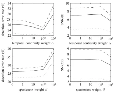
FIGURE 5.3– EFFECT OF DIFFERENT TEMPORAL CONTINUITY WEIGHTS AND SPARSENESS WEIGHTS ... 80
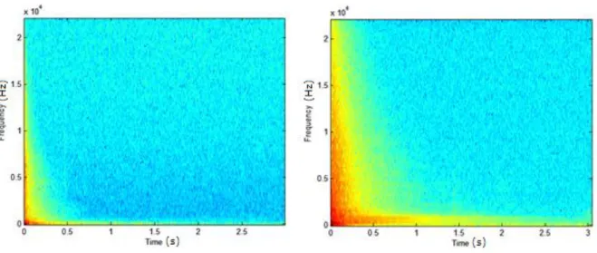
FIGURE 5.4–SPECTROGRAMS OF POWERFUL STROKES ON THE EDGE OF A SPLASH AND OF A CHINA CYMBAL ... 80
FIGURE 5.5–SPECTROGRAMS OF SOFTER STROKES ON THE EDGE OF A SPLASH AND OF A CHINA CYMBAL ... 81
FIGURE 6.1–CHOP CHOP STUDIO. ... 84
FIGURE 6.2–CYMBALS SAMPLED. ... 85
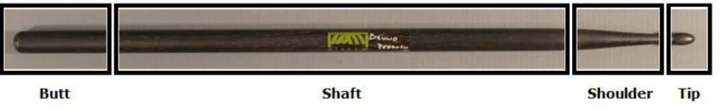
FIGURE 6.3–ANATOMY OF A DRUM STICK ... 86
FIGURE 6.4–SCATTER PLOT OF THE TRAINING SET FOR V.A. ON COMBINATION #1 OF TABLE 6.2. ... 90
FIGURE 6.5–IN GREEN THE POINTS FROM THE SAMPLE WITH LOWEST AMPLITUDE FROM THE CHINA ON COMBINATION #1………....91
FIGURE 6.6–SCATTER PLOT OF THE TRAINING SET FOR V.A. ON COMBINATION #3 OF TABLE 6.2. ... 91
FIGURE 6.7–IN GREEN THE POINTS FROM THE SAMPLE WITH LOWEST AMPLITUDE FROM THE SPLASH ON COMBINATION #3 ... 92
FIGURE 6.8–IN GREEN, POINTS FROM THE SAMPLE OF THE SPLASH ON COMBINATION #3 THAT WAS BADLY CLASSIFIED ON TABLE 6.2. .. 93
FIGURE 6.9–THRESHOLDS. ... 93
FIGURE 6.10–SOURCE SIGNALS FROM SPLASH AND CHINA OBTAINED BY NMF ... 96
FIGURE 6.11–SOURCE SIGNALS FROM 14 INCH CRASH AND 16 INCH CRASH OBTAINED BY NMF ... 97
FIGURE 6.12–SOURCE SIGNALS FROM CHINA AND 16 INCH CRASH OBTAINED BY NMF ... 99
13
Tables Index
TABLE 4.1–SNR RESULTS FOR VARIOUS TYPES OF SOUND SOURCE SEPARATION TECHNIQUES ... 51
TABLE 4.2– DECOMPOSITION RESULTS ... 56
TABLE 4.3–SNR RESULTS FOR VARIOUS TYPES OF SOUND SOURCE SEPARATION TECHNIQUES ... 56
TABLE 4.4– TABLE WERE PSA AND NSF ARE APPLIED TO SIGNALS ... 57
TABLE 4.5–SUB-BAND ISA TRANSCRIPTION RESULTS OF A DRUM LOOP ... 66
TABLE 4.6– COMPARISON BETWEEN THE RESULTS FROM APPLYING SUB-BAND ISA AND PSA TO THE SAME DRUM LOOP ... 733
TABLE 6.1–NUMBER OF SAMPLES AVAILABLE FOR ANALYZES... 87
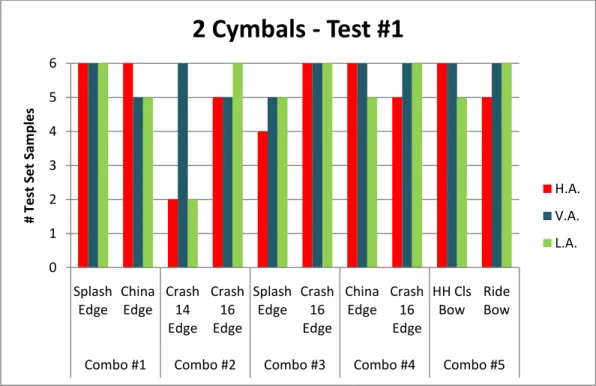
TABLE 6.2–TABLE WITH THE NUMBER OF CORRECTLY CLASSIFIED AND SEPARATED SAMPLES IN TEST #1 ... 89
TABLE 6.3–TABLE WITH THE NUMBER OF CORRECTLY CLASSIFIED AND SEPARATED SAMPLES IN TEST #2 ... 94
TABLE 6.4–TABLE WITH THE NUMBER OF CORRECTLY CLASSIFIED AND SEPARATED SAMPLES IN TEST #3 ... 95
TABLE 6.5–COMBINATIONS WITH HIGH AMPLITUDE TRAINING SETS AND WITH VARIABLE AMPLITUDE TRAINING SETS ... 98
TABLE 6.6–TABLE WITH THE NUMBER OF CORRECTLY CLASSIFIED AND SEPARATED SAMPLES IN TEST #1 ... 100
TABLE 6.7–TABLE WITH THE NUMBER OF CORRECTLY CLASSIFIED AND SEPARATED SAMPLES IN TEST #2 ... 100
15
1.
Introduction
Music is constantly present in our everyday activities. From the first second of our day when we wake up with the radio from our alarm clock, to the most common entertainment mediums like cinema, television, video games, and of course radio, to the music we ear and sing while bathing or while traveling to work. It is quite amazing how in just a few seconds after the start of a song we are able to recognize and identify it. However, recognition of a song or a piece of music does not enable a listener to transcribe it.
Transcription is the ability to identify and register instruments’, harmonic1
, rhythmic2, and melodic3 features of a piece4 of music, using standard staff notation5. It requires the
attainment of aural skills6 and music theory knowledge and comprehension, which are only
possible through training and study. To achieve a level of proficiency in transcription that is fast and accurate can take a long time. This way, for a beginner, several weeks may be required to transcribe only one of the instruments from a musical piece, without guaranties of total accuracy. Although not deprived of usefulness this ability enables little utilizations besides transcription and music composition.
1 Harmony deals with pitches that are played at the same time [Burrows 99]. The pitch of a note can be defined scientifically in terms of its sound waves frequencies. Similarly in music, a pitch is a fixed sound which can be identified using a series of letters ranging from A to G. So, every note you hear from a musical instrument has its own pitch [Burrows 99]. When at least three different notes sound together in the same instrument, the resulting effect is a chord [Burrows 99].
2 A pulsing effect that we feel when listening to a piece of music [Burrows 99]; usually its main engines are the percussion instruments.
3 Melody refers to the deliberate arrangement of series of pitches – what most people would call a tune [Burrows 99].
4 Throughout this thesis, music, song, and piece will be used interchangeably, refereeing to the same thing.
5 Staff notation consists of the written representation of all rhythmic, harmonic, and melodic elements in a piece of music. The notation is written in five lines which are known as the staff [Gerou 96].
16
If extended to a computer system (automatic) music transcription can be a very useful asset. It can be used in computerized music education as a learning aid for people wishing to learn how to play a piece of music where there is only access to an audio recording, and not the necessary skills to attempt transcription themselves. Areas of entertainment such as karaoke [Ryynänenm 08], music composition [Simon 08], and even song data base retrieval through humming - known as query by humming [Ghias 95], are some of the other potential applications.
Automatic music transcription (AMT) is a very hard problem to tackle, mainly due to representation issues. These are a result of music's many complex structures, which are a combination of mathematical (harmony, rhythm, and melody), and non-mathematical (tension, expectancy, and emotion) variables. Hence, computerized representations of these variables, along with the transformations used in audio processing, add even more to the complexity of this area [Dannenberg 93]. The number of note sources targeted for transcription, and the number of notes played at the same time are also detrimental to the accuracy of a transcription. When notes are played one at a time we are in the presence of monophonic music. On the other hand, if there is more than one note being played like a chord or when more than one instrument plays a note at the same time, we are in the presence of polyphonic music. Both monophonic and polyphonic transcription can be handled in a single or multiple instrument environments.
Salience, perception, pitch matching, complexity of a piece of music, and overlooking rhythm are discussed in [Byrd 02] as some of the most common problems of monophonic and polyphonic music regarding music information retrieval (MIR) for pitched instruments. A great deal of research on AMT is usually focused on pitched instruments. FitzGerald gives some possible justifications regarding the preference for this type of instruments [FitzGerald 04]:
17
Africa. It is also perhaps as a result of a feeling that the harmonic series of partials that go to make up a given pitch are easier to model than the noisy frequency spectra associated with most drum sounds.
However, over the last few years indefinite pitched instruments, mainly percussion instruments, started to garner more attention. From these, the one that stands out the most is the drum kit (see chapter 3.1 for more details on this instrument7), especially because of its increasing popularity in western music landscape. This growth in interested by the scientific community is also due to its usefulness in a great variety of musical situations where AMT is
needed. Query by beat boxing [Kapur 04] is one of them, it’s an information retrieval method
for music databases based on the same concept as query by humming, but seen primarily as applicable for Disk Jockey (DJ) usage. AMT of drum kit events can also be used as an aid for people wishing to transcribe the drum kit parts played in a song, or for studying this instrument. Producers and music lovers can also gain from the development of tools based upon AMT of the drum kit. If an audio recording has enough quality the drum track can be sampled8 to be used in other musical pieces. It is also possible to organize libraries of drum samples and drum loops by type of beat, tempo, or genre. Users with an enormous database of music could organize them by musical style based on the type of drum parts detected. Since some of the existing genres have a much defined rhythm structure, it is possible to label them based on that. Therefore, there is a whole world of new possibilities for the musician, the producer, and even for the everyday music enjoyer with AMT of drum kit events.
Most of the work on automatic drum transcription is focused on combinations of snare drum [Tindale 04], hi-hat, and bass drum (also known as the kick drum, these two names will be used interchangeably throughout the text) [Paulus 06, FitzGerald 06], which are the main
7 A drum kit is a collection of percussion instruments, so it is not accurate to call it an instrument. For simplicity and also because it is of common usage, and seeing that this issue is not relevant, in this dissertation besides drum kit we will also refer to it as an instrument and drum set.
18
instruments of a drum kit. To the best of our knowledge, transcription of elements like the open hi-hat or even the different cymbals has been neglected. Yet, an accurate transcription of drum kit events will never be possible without the transcription of different types of cymbals, and in the case of a hi-hat, if it is open, closed, or half-open (just to name a few possible uses of this instrument). The goal of this dissertation is to fill this void. Here we explore automatic cymbal classification9 and the identification of which class of cymbals the cymbal played belongs to. Classification is part of the transcription process. To perform correct transcription we have to first identify what instruments are being played, following this with detection of its positioning in the piece of music. We will focus on the five most used types of cymbal classes – crash, ride, splash, china, and hi-hat (for more information on each of these classes check chapter 3.2). Our study will only regard monophonic events from two or three cymbals played consecutively. Even though this work will only regard cymbal events, a great deal of issues will arise. From capturing all the dynamic nuances played by the drummer (strong or weak hits), classification of up to three cymbals played consecutively, to cymbals with different sizes, shapes, and timbres, these are some of the characteristics that will drastically increase the complexity of the work developed. Still, another problem arises from the typical harmonic series found in this type of instrument – it is harder to accurately classify a cymbal do to its noisy frequency spectra.
To steer our work in a good direction we chose to apply the cornerstones of the majority of information theory algorithms (IFA) – Principal Component Analysis (PCA) [Cavaco 07] [FitzGerald 04], Independent Component Analysis (ICA) [Abdallah 03] [Cavaco 07] [FitzGerald 04], and Non-Negative Matrix Factorization (NMF) [Smaragdis 03] [Hélen 05] [Moreau 07] [Virtanen 07], for sound source separation, combined with a classification algorithm for disclosing to what cymbal each sound sample pertains to. As we had predicted, PCA due to its constraints did not give satisfactory results. ICA’s results were also not very satisfactory, so we decided to focus our attention on NMF. This algorithm was chosen because of encouraging results when used as a standalone technique, as seen on [Smaragdis 03] and [Virtanen 07]. With NMF we were able to achieve a great level of success by
19
accurately classifying various combinations of two cymbals played sequentially, while with three cymbals the results were also very good, as with two cymbals.
We will start our journey by overviewing a collection of introductory topics. These range from the physical behavior of sound (chapter 2); physical characteristics and behavior of cymbals, and drum kit description (chapter 3). Afterwards, analysis and exploration of previous work will ensue with chapter 4 - State of the Art. There, we review several algorithms, their pros, and cons and possible applications to the problem at hand. Next, in the fifth chapter, we explain in detail the proposed system to solve our problem. This document will conclude with the analysis of the results on chapter 6 – Results and Discussion, and with the conclusions and future work on chapter 7.
This work was used as the basis for a paper with the title – Automatic Cymbal Classification Using
Non-Negative Matrix Factorization, written by Hugo Almeida and Sofia Cavaco, and submitted to an international
20
2.
The Physics and Math of Sound
As the reader may be aware of, for the development of a work of this magnitude a high level of study and research is needed. Thus, we start by reading the ones that preceded us, those who strived to success that paved the way. Through papers and thesis we are introduced to a new and very scientific world, with a whole new jargon for us to cope with, with a whole new set of rules. With all this in mind we will try our best to achieve the type of approach portrayed in [Eco 98]:
Once decided for whom to write for (for all mankind and not just for the evaluator) it is essential to decide how to write10.
We will write this thesis with one objective in mind, to always try to clearly explain all its content, independently of the level of knowledge of the reader. Thus, in an effort to elaborate a very comprehensive source of knowledge we will start by taking a look at how sound behaves and how digital systems can capture and mathematically represent sounds. If the reader is knowledgeable about the subjects studied in this chapter, he/she is free to jump over to the third chapter of this dissertation.
2.1. From Sound Wave to Waveform
Have you ever wondered how it is possible for a sound to travel from a speaker to your ears? Figure 2.1 is an illustration of what ensues, since a sound is emitted by a pair of speakers until it reaches our ears. The dots in the picture represent air molecules. The regions with great density of molecules are called areas of compression - where the air pressure is greater than the one from the atmosphere. On the other hand, the dispersed dots are areas of
21
rarefaction, regions where pressure is lower than the one exerted by the atmosphere. The small arrows in the diagram represent the movement of a sound wave through a channel, which is created by a translation of the compressed area inwards, as opposed to the outwards movement of the scattered air molecules [Everest 01].
Figure 2.1 – From [Everest 01], the effect of sound pressure on air molecules.
(A) – Sound pressure is responsible for air particles being pressed together in some regions, and sparse in others (B) – A small movement of the sound wave from the position occupied in A to a new one.
22
speaker to equilibrium, and displace the neighboring particles, which will enable the sound waves to move along the air. These movements are responsible for making the sound waves travel through the ear channel, which introduces changes in the wavelength of the sound wave. The end result of this is our perception of sound.
Now let us suppose that instead of reaching our ears the sound waves reach a microphone connected to a computer. In this particular case the information traveling in the sound waves will have to be digitized so it can be interpreted by a computer. When it comes to convert them to a digital medium their continuous information (in nature these waves are analog) will have to be transposed into discrete values. The digital and mathematical representation of the sound wave is called waveform, and is illustrated in figure 2.2 – B. This consists of representing the displacement of the air particles through time. In figure 2.2 we see the relationship between air pressure and the mathematical representation of a sound wave, where for example, values of compression represent high amplitude amounts. Now let us take a look at how the sound waves are translated into waveforms.
23
Audio digitization systems use time sampling and amplitude quantization to encode the infinitely variable analog signal as amplitude values in time [Pohlmann 00]. Samples are taken at irregular intervals from an analog signal to create a discrete signal. The number of samples recorded per second is known as sampling frequency.
This is enough to guaranty the reconstruction of a signal with the same frequency as the original one, if the sampling theorem is taken into consideration. This theorem defines the relationship between the analog signal and the sampling frequency, specifying that the sampling frequency must be at least twice the highest signal frequency in order to allow reconstruction of the signal. More specifically, audio signals containing frequencies between
0 and S/2 Hz (Nyquist frequency) can be accurately represented by a sampling frequency of S
samples per second [Pohlmann 00].
Figure 2.3 is a good visual example of what happens in the time sampling stage if the sampling theorem is followed. The samples will contain the same information as the original signal. Thus, the signal is reconstructed without loss of information [Pohlmann 00]. If the sampling theorem is not respected, information from the original signal will be lost, and it will not be possible to have the original signal reconstructed accurately in the discrete signal [Pohlmann 00]. As you can see in figure 2.4, the sampling frequency (44 kHz) is not two times the frequency of the analog signal (36 kHz) (figure 2.4 - A). This will in turn originate a deficient sampling frequency (figure 2.4 – B) blocking any possibility of an accurate reconstruction of the analog signal into a discrete one (figure 2.4 – C).
Since the machine representation of amplitude is limited by the number of bits used, the amplitude of each sample must be quantized, that is, the actual amplitude of the sample is
rounded to be converted to a k bit number. Because amplitudes can have a high number of
24
25
Figure 2.4 – From [Pohlmann 00], the effect of not obeying the sampling theorem. (A) – The orginal signal. (B) – The stored samples.
(C) – The inaccurate representation of the reconstructed signal.
2.2. Spectrograms
After the sound has been digitized into a computer it is possible to perform operations that enable a better retrieval of information for analysis. One of these operations is known as Fourier Transform (FT), a mathematical tool that enables decomposing time signals (such as waveforms) into the frequency domain. The discrete Fourier transform (DFT) is used instead of the FT to obtain a sampled spectrum for discrete time signals of finite duration. Just as the FT generates the spectrum of a continuous signal, the DFT generates the spectrum of a discrete signal expressed as a set of related sinusoids. The DFT takes samples of a waveform and operates on them as if they were an infinitely long waveform comprised of sinusoids [Pohlmann 00]. So with DFT it is possible to demonstrate that a sound input may be described as the combination of various other sinusoids. Nonetheless, the DFT is not a very efficient computational technique when compared to fast Fourier transform (FFT) [Burrus 08], so this last one is used instead.
26
do we hear natural sounds with a constant value of frequency through time, and as such we must use another method to better analyze their time-varying frequency content. To do so the input signal can be divided in windows with a time based function performing FFT on each one of the windows. This technique is named Short-Time Fourier Transform (STFT) which specifies magnitude versus time and frequency for any signal [Cohen 95]. Even though the FFT (and consequently the STFT) also give information about the initial phase of the frequency components of the waveform, here we will not make use of this information; we will only use the magnitude information.
A windowing function is illustrated in figure 2.5. This signal is broken into chunks that are multiplied by the windowing function, which is embodied by the series of red curves that are applied to the signal being analyzed and represented in blue. Afterwards, the results of applying FFT to each window can then be placed together in a single matrix called a spectrogram, which is a graphical display of the magnitude of STFT.
Figure 2.5 – From [ECE 10], short-time Fourier transform.
In equation 2.1 the spectrogram is represented in matrix where is an amplitude value at
time frame and frequency bin . In this following example (figure
27
intensity. The greatest value possible is dark red. From there, the amplitude value will decrease until it reaches the lowest level in the purple area.
(2.1)
28
3.
Drum Kit and Cymbals
This chapter gives a brief overview of the different instruments that are included in the most typical drum kit setup, and of the different families of cymbals we intend to use in this work for analysis purposes. Since each drum and cymbal has its own characteristics and voice, it is of the utmost importance to cover their functions as an instrument in the drum set, and in the case of cymbals, the sound differences between them. This is the most important goal of this chapter; educate the reader in the sound differences between each class of cymbals, and how their very audible differences can actually translate into very hard characteristics for IFA to perform sound source separation accurately. This chapter will also serve as a very basic educational resource for those who would like to expand their knowledge on important sound features to consider when using feature based classification for cymbals.
We have also included a brief historical background on cymbals on the Attachments. This serves to show the importance of these instruments in different elements and eras of mankind’s history, and how they evolved through time, helping to mold musical landscape from past and present alike. This further legitimizes the work developed for this dissertation, due to the level of historical and musical relevance of cymbals.
3.1. Drum Kit
29
Figure 3.1 – A basic rock/pop drum kit.
The snare drum, bass drum and hi-hat are the pieces that define the essence of a drum kit; they are the main instruments in almost all types of music. Jazz is an exception, since the ride cymbal has a more important role than that of the hi-hat. The remaining instruments are important as well but will depend mostly in the style of music played, and on the drummer’s personal preference. The importance of these four pieces of the drum kit is due to them being mainly used to keep time during songs, playing beats and embellishments that complement the song. Since time keeping is the most important role of a drummer, these four instruments become essential. The toms are used more often for fills, which are rhythmic patterns played in between sections of songs (e.g., between verse and chorus). They prepare the listener and the band to the next section. They can also be used in beats, just like the snare, bass drum, hi-hat, and ride can be used in fills, but that is not their main functions.
3.2. Cymbals
30
to get three unique types of sounds from the cymbals. Those areas are the edge, bow, and bell (figure 3.2).
Figure 3.2 – The different zones to hit on a cymbal.
Each cymbal family’s name is very recent. A catalog from 1948 of one of the most famous cymbal companies of our time, Zildjian, did not state their cymbals as being crash or ride, but distinguished them by their sizes (7 to 26 inches) and weights (Thin, Medium, and Heavy, just to name a few). In the next sections we will be taking a look at each class of cymbals that will be used for the analysis stages of our work. Here we introduce each class’s origins, mains usages, and playing techniques. We will also get to discuss how their physical features forge the aspect of their respective spectrograms and sound. The next sections are based around the various chapters that can be found on [Pinksterboer 92].
3.2.1. Hi-Hat
31
Figure 3.3 – A Hi-Hat.
The hi-hat is a very versatile instrument that enables the usage of a great number of techniques. When the pedal is pressed down the two cymbals are squashed against one another, this is the closed position or closed hi-hat (figure 3.3). When the pedal is not pressed down the two cymbals will have some distance separating them. This is called the opened position, or open hi-hat. The most common sizes for a pair of hi-hats range from 10 to 15 inches.
There are other techniques utilized with this cymbal like the “foot chick”; when the pedal is pressed down by the foot and a “chick” is heard as a result of the two cymbals hitting each other and closing the space between them; the “foot splash”, when the pedal is pressed and the two cymbals touch each other for a little fraction of time, returning promptly to the opened position.
32
due to both cymbals rattling against each other with any stroke, but with a longer decay spread equally through the frequencies.
Figure 3.4 – Spectrogram of a hit on the bow of a Hi-Hat.
33
Figure 3.5 is the spectrogram of a piano note. It gives us the fundamental frequency as the line with a higher level of energy, and the remaining harmonics from the note played. The difference between figures 3.4 and 3.5 is astonishing. In figure 3.5 instead of covering the entire human frequency range like on figure 3.4, we get very well defined bursts of energy. This is something common to any piano note. This way, it is harder to distinguish between the different cymbals than it is to distinguish between the different notes played on a piano.
3.2.2. Ride Cymbal
The name of this cymbal derives from what is played on it, steady, rhythmic, and driving patterns called ride patterns. That is why most drummers like to play this cymbal in the bow or bell areas, since these are the regions where we can get a more defined sound for playing the ride motifs. It is possible to find rides (figure 3.6) with sizes ranging from 18 to 24 inches. They are usually very heavy and thick, making their sound louder, compact, and much defined.
Figure 3.7 shows spectrograms of strong hits on both bell and bow areas of this cymbal. Taking a closer look at the spectrogram, we can see that the low frequency range (below 500 Hz) has a much longer decay. This is due to a couple of aspects - higher frequencies have a faster decay, low frequencies tend to last longer, and because all cymbals, when stricken, have an initial explosion that is rich in low frequencies. This does not mean the sound of this cymbal will be very low. However, due to their size and weight, ride cymbals tend to be lower pitched when compared with a crash cymbal, for instance, and as such have longer decays.
34
to the edge) evenness11. All these factors contribute in one way or another for the overall decay of the cymbal. We would need a lot more information and study to be able really evaluate what is influencing the decay of both bell and bow. In comparison to the spectrogram of figure 3.4, these ride spectrograms are way more readable. They are still very noisy when compared with the one on figure 3.5.
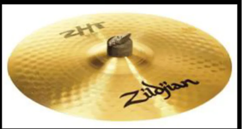
Figure 3.6 – A Zildjian ZHT 20 inch Ride Cymbal.
Figure 3.7 – (Left) Spectrogram of a hit in the bow of a ride. (Right) Spectrogram of a hit in the bell of the ride.
11
35 3.2.3. Crash Cymbal
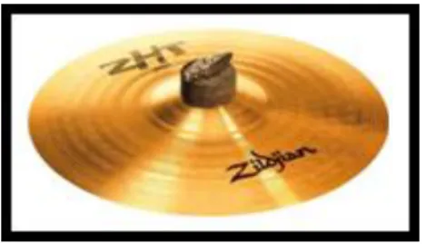
After the development of the first ride cymbal, the smaller and lighter cymbals whose objective was of playing accents in a song by hitting their edges, eventually got named crash cymbals. These cymbals have a quick decay due to their usually thinner taper and lighter weight. The most common sizes for this type of cymbals are in the between 14 and 20 inches (figure 3.8), with the edge being the most played area of this type of cymbal.
Figure 3.8 – A Zildjian ZHT 14 inch Crash Cymbal.
36
Figure 3.9 shows the spectrogram of a crash cymbal when struck on the edge. When hitting this cymbal on the edge (known as crashing) the effect is a little different than when playing on the bow or edge of the ride. In the case of the crash, which is usually a much lighter and thinner cymbal than a ride, by striking its edge we will get more overtones, and a less controlled and defined sound. The decay is faster but the sound is explosive. Just like with the ride cymbal, the low frequency range has a much slower decay, with the higher frequencies having a faster decay, and low frequencies tending to last longer. However, there are a lot higher frequencies being excited here and with a longer decay than what we saw with the ride. Once again this is due to the weight and thickness of crash cymbals.
3.2.4. Splash Cymbal
These cymbals can be considered as small crash cymbals as can be seen on figure 3.10. Their sound is fast and bright, with a short sustain. Just like the crash cymbals, they are usually used for short accents. The most common sizes for splash cymbals are in between 6 and 12 inches.
Figure 3.10 – A Zildjian ZHT 10 inch Splash Cymbal.
37
Figure 3.11 – Spectrogram of a hit in the edge of a Splash Cymbal.
3.2.5. China Cymbal
China cymbals where very popular at the beginning of the 20th century, and were used mainly
as a ride cymbals. In the early 1970’s drummers started to use them more and more as additional crash cymbals. Like the name states, these cymbals came originally from China, and have a very characteristically flanged edge just like the cymbal of figure 3.12. The cymbal on the picture maintains very few resemblances with the original Chinese cymbals however, besides the flange.
38
Figure 3.13 – [From Pinksterboer 92] Profiles of various types of china cymbals.
Original Chinese cymbals had a conical bell or handle, since these bells were used to be grabbed so a percussionist could crash a cymbal against each other. The western counterparts of the Chinese cymbals usually have a normal bell or a square one. Figure 3.13 shows the various shapes of china cymbals that can be found.
The sounds of some of the original Chinese cymbals resembled the sound produced by trash can lids. The western variations of this cymbal however are more pleasing to the ears, with a much warmer and harmonic sound. Nowadays these cymbals are most commonly used in the same manner as crash cymbal, but with an exotic sound to it; continuing a trend started in the seventies. Some drummers rather use it as a ride just like the first western drummers who used them. Due to its shape it can also be played in very different positions, whether facing up or flipped over. In this last position the bell of the cymbal cannot be played.
39
the sound of a china can be. The same rules we have been talking about with all the other cymbals apply here also.
Figure 3.14 – Spectrogram of a hit on the edge of a China Cymbal.
40
4.
State of the Art
Most classifiers studied for dealing with musical instruments are directed towards string and wind harmonic instruments. Still, some of these studies focus on the recognition of different types of strokes in percussion instruments with indefinite pitch, like the snare drum and conga drums [Bilmes 93][Schloss 85][Tindale 04]. However, most of the studies focus on identifying different instruments from the drum kit - bass drum, snare drum, hi-hat, toms and cymbals [FitzGerald 02][FitzGerald 04][Sillanp 02][Herrera 02][Gouyon 01][Paulus 06][Moreau 07]. Nonetheless, some of the proposed classifiers cannot clearly distinguish between the classes of cymbals. This means the sounds from any of the cymbals in the drum kit are assigned to the same class - cymbals.
Sound classifiers have two different stages, one for sound features extraction and another for classification. Many low and high level temporal, spectral and short-time features have been used to try to typify indefinite pitch percussion instruments. However, many classifiers give use to a blend of various features for getting good classification rates [Bilmes 93][Gouyon 01][Kaminskyj 01][Paulus 06][Schloss 85][Sillanp 02][Tindale 04]. This happens because of the issues that arise when deciding the most appropriate features to characterize the data. While most sound classifiers use a set of pre-defined features, others are that learn the features using decomposition methods such as ICA, ISA, Sub-band ISA, and NMF [FitzGerald 02][FitzGErald 04][Moreau 07], which we will be studying next, among another methods such as these.
4.1. Decomposition Methods
41
function? After a while we realize that it is a very obvious answer - it is its shape, because even if we used a chair as a table for one hundred years, it would still be a chair being used as a table. But still, what is the principle that guides our assessment of reality that makes us decide that some object has a certain denomination?
When trying to figure out what defines a chair, we use inductive reasoning, i.e., an intellectual and conscious effort; however, to start this whole process of intellectualizing the chair, we have to first learn what a chair is. This is accomplished by perception [Attneave 54]. Perception is a sensorial mechanism that enables an inner representation of the outside world as well as its understanding. It enables us to react in the best possible way regarding external stimuli, having our own preservation as its main goal. Thus, speed on the perception of our surroundings is of the utmost importance. This can become a real problem to achieve, since we are constantly being bombarded with sensorial stimulus, and storing it all would be a total waste of space, since a great slice of our everyday stimulus is redundant, that is, accurately predictable and whose knowledge has already been acquired [Barlow 01]. But should the entire redundant stimulus be ignored to achieve a best level of comprehension about the new stimulus?
Barlow postulates that the perception of sensory messages may have a certain degree of redundancy and loss of information [Barlow 59], and that a total level of compression, that is, no redundancy whatsoever, is not the way our brain handles sensorial information. Without redundancy it would not be possible to identify structural regularities in the environment, essential to survival [Barlow 01]. This work developed by Barlow on quantification of information is called information theory. This discipline is instrumental in presenting compression techniques and redundancy reduction algorithms, not only useful in understanding how our brain functions, but in performing computer driven operations like image compression and sound source separation. A very well known case of sound source separation is described next.
42
sources in the form of conversations, and engaging our ears as one single stream of cacophony, we call a signal mixture. Although some masking can occur, it is possible to concentrate on just one of those dialogues and separate it from the rest. This is known as the “cocktail party effect” [Arons 92] and is a problem of blind source separation (BSS). It is called BSS because there is an ability of separating a conversation from the mixture of dialogues without knowing the sources [Plumbley 02].
BSS is what we intend to perform in this work, but instead of separating one dialog from a stream of cacophony, we intend to identify to which class consecutively played cymbals in a signal mixture belong to. BSS based techniques use waveforms as inputs. Each one of the waveforms represents one source signal, and each source signal is a mixture of the sounds coming from the different sound sources. For each sound source there is a microphone recording the surrounding sounds. Now for our case, instead of using various waveforms we will use only one but represented by a spectrogram. A spectrogram can be assumed to be the
result of the sum of an unknown number of independent source signals, each represented by
an independent spectrogram. So in this chapter we take a look at some algorithms’ potential
to perform separation of sound sources form a spectrogram of a mixture of various cymbal samples.
FitzGerald made a very comprehensive study on the separation and classification of the
standard rock/ pop drum kit’s main instruments (check chapter 3.1 for more information on
the rock/ pop drum kit). For that goal he used several algorithms, such as PCA, ICA, Independent Subspace Analysis (ISA), Sub-band ISA, and Prior Subspace Analysis (PSA), which we will explore in more detail below [FitzGerald 04]. Other promising techniques we will also explore include NMF and Non-Negative Sparse Coding, since they seem of great usefulness regarding cymbal separation.
We will start by analyzing PCA, ICA and NMF – that can be used as blind source separation
43
ISA, and Sub-band ISA. We will end this chapter with the analyzes of Locally Linear Embedding (LLE), an algorithm that can substitute PCA in techniques like ISA and Sub-band ISA, and with PSA.
4.1.1. Principal Component Analysis
PCA is a method used primarily for redundancy reduction or dimension reduction, i.e., data compression, and can be used to find patterns in high dimensional spaces. This is accomplished by finding an ordered set of uncorrelated Gaussian signals, such that each signal accounts for a decreasing proportion of the variability in the set of signal mixtures, where this variability is formalized as variance [Smith 02].
PCA starts by subtracting the mean from the N-dimensional mixtures in order to produce a data set with zero mean [Smith 02] (i.e., it centers the data at the origin of the N-dimensional space). Figure 4.1 illustrates this; on the left image we have the original N-dimensional mixture, while on the right we can check the result of subtracting the mean from the mixture. By not going along this line of procedure, the best fitting12 plane will not pass through the data mean but instead through the origin [Miranda 07]. Once the data is centered PCA searches for the areas of greater variability, so that from a set of signal mixtures x, it can get a set of extracted/source signals y, that is, PCA tries to unmix the signal mixtures.
Lets us take as an example a 2-dimensional space, and two signal mixtures and . From
these mixtures it is possible to extract two source signals and . For a successful extraction it is required to use an unmixing coefficient for each mixture. In this next example we use two of them, a and b, to extract like so:
(4.1)
This pair of unmixing coefficients defines a vector:
12
44
(4.2)
Figure 4.1 – From [Smith 02], Mean adjustment of the N-dimensional Space On the left, the original mixtures on a 2-dimensional space.
On the right, the mean adjusted 2-dimensional space for the mixtures.
This vector has two very important geometric properties - length and orientation. Length defines the size of the amplitude of the extracted signal, making it bigger or smaller. Orientation is the factor that enables extraction of the signal. Let us call to the space
defined by the source signal axis and , and by the space defined by the signal mixture
axis and [Stone 04]. Both these spaces are defined in figure 4.2.
To unmix the signal mixtures we start by factorizing the mixtures by the employment of singular value decomposition (SVD). This technique decomposes a matrix into several component matrices that are often orthogonal or independent [Ientilucci 03]. The factorization goes like this, with C being the mixture matrix,
45
U is a matrix with basis on the columns; S, a diagonal eigenvalue matrix; and a matrix
with time based source signals on the rows. The column vectors of and line vectors of
are eigenvectors; with a related eigenvalue on the diagonal matrix . Each of these vectors works just like the unmixing coefficient , representing a line of best fit through the data mixture that finds uncorrelated Gaussian signals from it. Uncorrelation is assured by the orthogonality between the directions of the eigenvectors. Figure 4.3 has perpendicular vectors in red assuring uncorrelation, while the transformed axes are drawn as dotted lines.
Figure 4.2 – From [Stone 04], source signal axis (left) and signal mixture axis (right).
Sorting the eigenvalues in descending order yields the same ordering for their respective eigenvectors on both U and V [FitzGerald 04]. This way, we will have the eigenvectors ordered from greatest to lowest value of variance [Smith 02]. This will enable us to perform data compression by removing the eigenvectors with the lowest values of variance, since lower variance dictates a less relevant eigenvector when it comes to the overall signal strength and idiosyncrasy.
46
Figure 4.3 – From [Stone 04], PCA of two speech signals. Each solid red line defines one eigenvector.
FitzGerald tested the use of PCA on spectrograms of drum sounds mixture. The information
available on the spectrogram of the mixture is represented by a matrix with
signal mixtures. It is possible to learn a unmixing matrix that allows extracting
independent source signals from :
, (4.4)
where is a matrix that contains the independent source signals. With
, equation 4.4 can be rewritten as:
(4.5)
47
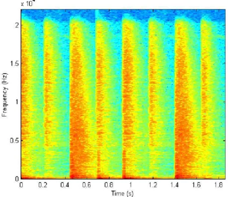
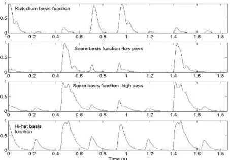
Figure 4.4 shows the spectrogram of the drum loop FitzGerald used. It contains sounds from snare drum, kick drum, and hi-hat. After performing PCA on the spectrogram we get a set of frequency basis functions. Figure 4.5 shows the first three basis functions, while on figure 4.6 we have the first three source signals. Each of the basis functions are related to any of the source signals; for instance, the first basis is related to the first source signal. This means that the source signals are the coefficients in a new dimensional space defined by the basis functions. The first frequency basis function is related to the whole signal, while the second and third show only information regarding the kick drum and snare drum sounds [FitzGerald 04].
Figure 4.4 – From [FiztGerald 04], the spectrogram of a drum loop containing snare drum, kick drum and hi-hat.
We have a basis for snare drum and bass drum, but what about the hi-hat? This instrument has a very low amplitude level, so its variance is also low and the source signals that only have hi-hat information are ranked low. Clear information regarding hi-hats can be found only after five source signals [FitzGerald 04].
48
enough. There is no guaranty that it will separate the different sound sources in the mixture into separate source signals. This feature by itself is enough to discourage the use of PCA on cymbal separation.
The separation of each drum kit instrument through different basis was unsuccessful. This can be confirmed by the second and third basis functions and source signals of both figures 4.5 and 4.6, where information regarding both kick and snare is scattered through them. So even though PCA seems deemed to failure, there are ways of improving its overall success when separating the different sound sources from the mixture.
Figure 4.5 – From [FiztGerald 04], the first three basis functions.
Onset detection13 could be used for the separation of each drum instrument through the search of abrupt increases in the energy envelope of the coefficients with the various basis [Hélen 05]. Afterwards the separated coefficients related to one specific drum kit piece could be joined in a single source signal. Anyhow there still remains a big problem, how to detach
49
coinciding events? Since this type of algorithm does not use prior knowledge but accumulated experience from the input, like we will see in NMF, if there are no isolated events that represent each of the drums in the coinciding event, separation is not possible [Smaragdis 03].
As we have seen, PCA favors basis of high amplitude. The information from sounds of low amplitude, like from the bow of the ride, or from a closed hi-hat can be represented by basis functions of very low rank.
Figure 4.6 - From [FiztGerald 04], the first three source signals.
4.1.2. Independent Component Analysis
50
When the mixtures are represented as waveforms, ICA requires having at least the same number of mixtures, that is, signals from different sound sources, as sound sources. For example, if we have two distinguishable sound sources, placing two microphones in two distinct places will create two different mixtures, since different distances of each sound source from the microphone will enable different proportions of the two signals in each mixture. Microphone placement works in the same way as camera placement. With an increased number of cameras filming a particular scene from different angles, we will get a much complete notion of what his going on. This way it will be possible to describe the scene with a greater level of detail [Stone 04]. However, when the sound of a drum kit is
recorded in a studio14 and ultimately mixed into a sound file, usually we get a maximum of
two channels (stereo) from where we can separate the different cymbals used. Taking into account that we usually have at least three cymbals in a drum kit, ICA is doomed to failure if only two channels are available. To outflank this, another procedure can be used; much like PCA it is possible to apply ICA to the spectrogram of a sound mixture. Nevertheless with ICA the dimensionality of the data can be reduced by considering only source signals,
where [Cavaco 07].
To build the unmixing matrix it is required to use unmixing basis, one for each mixture. Thus, equations 4.1 and 4.2 are applicable here as well, and in the same molds, i.e., which will be an unmixing basis in , defines a weight vector used in the signal mixture space. Its length defines the size of the amplitude of the extracted signal, making it bigger or smaller. While the unmixed sound sources may be recovered, their original magnitude level can differ from the original signal. Orientation is the factor that enables extraction of the signal [Stone 04]. For a weight vector to extract a source signal it will have to be orthogonal to the orientations associated with the rest of the source signals, except the one that it will
extract. In figure 4.7 we can see that by being orthogonal to , will be able to separate
source signal , like stated.
14
51
Figure 4.7 – From [Stone 04], w1 orthogonal to all source signals (S2) except S1.
Table 4.1 – From [Helen 05], SNR results for various types of sound source separation techniques.
52
the noise is over the signal, thus we have a greater level of success on the separation. The SNR obtained with all the methods are low, with ICA having the lowest value of them all, as can be seen on table 4.1. Other techniques like NMF, and under the same conditions, showed better performance than ICA when separating percussion instruments from the original mixture, in which cymbals were included.
4.1.3. Non-Negative Matrix Factorization
The base concept behind NMF is the same as the one seen on PCA and ICA. Nevertheless, rather than establishing statistical independence or uncorrelation as the basis for this factorization process, NMF uses non-negativity. This technique has a matrix notation similar to the one in equation 4.5, and can also be applied to the spectrogram of a mixture. Matrix of size is comprised of a set of N-dimensional data vectors, which are placed in its columns, with signal mixtures in the rows. This matrix is then factorized into of size
where its columns are the basis functions, and of size ( , with source signals. This factorization is conceived in a way that makes it possible for the new matrices
to be smaller than , since , which may result in data compression [Lee
01]. As we will see further down in this section, this can bring about some complications regarding the level of success of the factorization.
With the non-negative constraint. NMF does not allow negative values in any of the component’s magnitude spectrums, enabling the components gains to be addictive between them. With this we have a parts-based representation, one that enables the different components to act like different parts of a source signal, without subtracting information between them to build the whole [Lee 99].
53
that with NMF the reconstruction of the original facial image loses its original magnitude values. This is shown by the levels of gray on figure 4.8, where these levels are different
between the original image ( ) and its reconstruction ( ). The original face is reconstructed
accurately using the basis matrix, although being mostly an approximation of the original data.
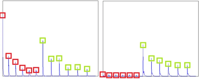
A good example of using NMF for sound source separation comes from [Smaragdis 03]. Smaragdis and Brown performed a study on the transcription of a polyphonic music signal using NMF, where polyphony events were two notes played from one instrument at the same time and by the same instrument. This algorithm was tested over recordings of a piano, with both isolated and coinciding notes played. On figure 4.9 we can see a series of isolated notes and only one polyphonic event, which is surrounded by a red box.
Figure 4.8 – From [Lee 99] NMF applied to face representation.
54
This musical piece has ten events with seven different notes, so let be seven ( ). The result of NMF of this musical piece can be seen on figure 4.10. On the left image we have the representation of the values in matrix (source signals), and on the right the values in matrix
(basis functions). On the third row of we can observe a source signal filled with noise, which signals a non-note source signal. This non-note source signal is the result of setting to seven, but having NMF consider that there are only six events. This means that one of the sources has two notes in it that are regarded as one event, instead of two. The notes we are talking about are the ones played at the same time in figure 4.9. You can locate them on the sixth row of of figure 4.10.
Since NMF does not use prior knowledge, the only way to achieve a comprehensive and correct transcription result is through accumulated experience from the input [Smaragdis 03]. Thus, for this technique to be able to separate those two notes in the mentioned sixth row, both of them have to be part of the musical piece as unique events also. Separation is not possible in this case since these two notes are always played at the same time in the input signal.
With this algorithm it is not possible to know exactly how many source signals are to be retrieved from the input signal without prior study of the musical piece. Setting a value for will condition exactly how many source signals to be returned. If the value chosen is less than the number of notes in the input then information will be lost and exact reconstruction will not be possible. On the other hand, if is greater than the number of notes available, the coefficients (notes) with greater level of energy can be distributed amongst the rest of the
entries in and . Ergo, the choice of a random value for is not quite effective unless we
know how many sources we want to retrieve from the input.
55
overall hit rate ( ) was calculated as the mean of individual instrument hit rates [Moreau 07]. Probably the most noticeable aspects of this table are the results regarding the hi-hat, which are the worst from the bunch. The overall results were very poor, probably due to the test data utilized, since only a song of one minute long was used to test the system [Moreau 07].
Figure 4.10 – From [Smaragdis 03], Decomposition of a musical piece.
NMF capacities were also tested along a system designed for the separation of a polyphonic musical signal into two classes - drum kit and pitched instruments [Hélen 05]. To achieve this goal the input signal was first separated into source signals using NMF. Afterwards support vector machines (SVM) classified sources according to one of the classes they
belong to – harmonic instruments or drums. Results were evaluated using SNR. In the signals
56
Table 4.2 – From [Moreau 07], decomposition results. Rp – Precision Rate/ Rr - Recall Rate/ Rh – Instrument Hit Rate
Table 4.3 – From [Helen 05], SNR results for various types of sound source separation techniques. In red the results of applying NMF of separating the drum part.
The last case studied was presented by Paulus and Virtanen [Paulus 05]. It consists of three stages. In the first one, source signals are estimated from training material for each instrument in the mixture. The training material comprises samples for unique sounds of each cymbal. NMF is applied to each sample for any instrument. The basis functions for samples pertaining to a given instrument are then averaged over the total number of samples for that cymbal in the training set hailing the instrument’s source spectra. This procedure is repeated for all instruments [Paulus 05]. In the second stage each drum instrument is separated from the mixture using the training source spectra. In the last stage of the algorithm, onset detection is applied to determine the temporal locations of sound events from the separated Signals [Paulus 05]. As usual, snare drum, kick drum, and hi-hat were used for this test. In table 4.4, precision rate ( ), is the ratio of correct detections to all detections; recall rate ( ) is the ratio of correct detections to number of events in the reference annotation. The
overall hit rate ( ) was calculated as the mean of individual instrument hit rates. Avg is the
57
by the number of instruments, B (bass drum), S (snare drum) and H (hi-hat). NMF presents
better results than PSA15, especially on the hi-hat. So this algorithm may perform very well
against cymbals.
Table 4.4 – From [Paulus 05], table were PSA and NSF (Non-negative spectrogram factorization – NMF applied to a spectrogram) are applied on an unprocessed signal (left)
table were PSA and NSF are applied on a processed signal (right).
The results of the analysis in [Moreau 07] although substantially weak, especially with the hi-hat, are insufficient to reach a conclusion, since only one test signal was used. On the other hand, the methods used in [Smaragdis 03] were successful in their separation efforts. Nonetheless they were not able to separate notes played at the same time. The only way to achieve separation with NMF is if both notes are part of the musical piece as unique events also. The notes played at the same time are one event, and is with events that NMF works. Like Smaragdis, Helén and Virtanen in [Helén 05] had a certain degree of success in proving that NMF could be effective in separating drum signals from polyphonic signals in a way that helped the classifier hail very good results, with a success rate of 93%. What is most encouraging is that besides considering the usual drum kit pieces for separation, cymbals were also added to the mix. The results in [Paulus 05] are very encouraging. AS you will able to see in section 4.8 of this chapter, PSA has very good results in what concerns separating bass drum, snare drum, and hi-hat from a mixture. However with NMF the results are even better, and the hi-hat, which is the cymbal that could be the most neglected here,
15
58
actually has a success rate of 98% for unprocessed signals, and of 96% for processed signals, which is quite astonishing.
With the results shown here it is possible to admit that NMF may be a suitable algorithm to perform cymbal separation with some level of success. We don’t have cymbals samples being played at the same time (they are played sequentially in the same sound file), so the issues found on [Smaragdis 03] may not occur. We also use a classification algorithm over the sound sources separated from NMF. Since in [Helén 05] we have a 93% of success when using a combination of NMF with a classification algorithm, and a 98%/ 96% of precision ratio for hi-hat detection, once again, from these results we expect this to be a very good option for classifying cymbals accurately from the mixture.
4.1.4. Sparse Coding and Non-Negative Sparse Coding
Sparse coding was intended to be a coding strategy that would be capable of simulating the receptive fields of the cells of the visual cortex of mammals [Olshausen 96]. Sparse coding considers that at a given moment only a certain number of sources are active, which means that only a certain number of sources are responsible for the creation of each observed signal [FitzGerald 04]. In order to identify the source signals sparse coding has to find the set of basis functions that enables the greatest level of independency amongst the source signals.
Olshausen conjectured that an image could be described with only a few coefficients out of the full set. To achieve this a form of low-entropy16 should be found. If low-entropy is applied to all source signals, a lower level of dependencies can be achieved between them, enabling a greater level of sound source separation [Olshausen 96], and a greater level of independency. We first talked about independence when we introduced ICA for the first time, thus is there any kind of relationship between ICA and sparse coding?