http://dx.doi.org/10.1590/S1982-21702014000200025
USING A LEAST SQUARES SUPPORT VECTOR MACHINE TO ESTIMATE A
LOCAL GEOMETRIC GEOID MODEL
Uso do método “support vector machine” por mínimos quadrados para estimar um modelo geométrico local para o geóide
SZU-PYNG KAO CHAO-NAN CHEN
HUI-CHI HUANG YU-TING SHEN
Department of Civil Engineering, National Chung Hsing University, No. 250,Kuo Kuang Road, Taichung, Taiwan
ABSTRACT
Keywords: Least Squares Support Vector Machine (LS-SVM); Kernel Function, Local Geoid Model.
RESUMO
Este estudo empregou pontos de controle de GPS em regiões-teste com altitudes ortométricas de primeira ordem previamente conhecidas, para a obtenção de pontos de coordenadas planas e altitudes elipsoidais, com a utilização do método cinemático em tempo real (RTK). Este estudo aplicou o ajuste de superfície de primeira ordem, ajuste de superfície de segunda ordem, método da retropropagação para redes neurais e “support vector machine” por mínimos quadrados (LS–SVM). Integridade e localização de dados foram examinados, e a certa quantidade e distribuição de pontos de referência modificados para obtenção da solução ideal. O estudo contou também com o LS-SVM e com o modelo de altitude geoidal local que foi estabelecido usando 3 funções de Kernel para análises e pesquisas. Os resultados indicam que a precisão total dos valores calculados das ondulações geóidais geométricas locais usando a rede neural artificial e o polinômio de terceira-ordem da função de Kernel foram ideais com o valor quadrático médio de aproximadamente ± 1.5 cm. O resultado mostrou que o SVM oferece o método rápido e prático para obtenção de altitudes ortométricas e provê a pesquisa acadêmica de referência para modelos geoidais locais.
Palavras-chave: Máquina de Vetor Suporte para Mínimos Quadrados; Função de
Kernel; Modelo de Geóide Local.
1. INTRODUCTION
If engineers can leverage GPS survey techniques to establish a precise local geometric-geoidal model and a system for converting ellipsoidal and orthometric heights, the traditional leveling survey model can be modified, improving measurement operations. The current geoid establishment methods comprise the astrogeodetic and astrogravimetric leveling, gravitational field model, and mathematical function-fitting methods (ABDALLA et al.,2011; AKCIN and CELIK, 2013; FEATHERSTONE et al.,2004; KAO and SHEN, 2011;Kao et al., 2010; KAO, 2006; KAO and BETHEL, 1992(a) 1992(b); LIN,2007; SHEN, 2011; TRANE Setal., 2007; USTUN and DEMIREL, 2006; WANG, 2005; YOU, 2006; YANG, 1999). If local geoid changes are smoothed within a certain range, then mathematical functions can be used to reflect the spatial distribution conditions. In the mathematical function-fitting method, GPS technology is employed to measure sufficient control points ina survey area and the ellipsoidal heights are derived based on local ellipsoids. The orthometric height is determined using direct leveling surveys. If the vertical deflection influence is disregarded, local geometric-geoidal undulations can be derived by subtracting the orthometric height from the ellipsoidal height of a location, enabling a partial simulation of the geometric geoidal undulations between the local geoid and ellipsoid by using a mathematical function-fitting method. In this study, the GPS control point of a test region involving known first-order orthometric heights and GPS real-time kinematic (GPS RTK) measurement method were used to calculate the plane coordinates (x, y) and ellipsoidal height (h) of the survey point. Various fitting calculation methods and fitting points were used to determine the optimal resolutions of each fitting method. Integrality and localization were discussed, and an accurate local geometric-geoid model was used to achieve local geometric-geoid calculations. The study was executed in the Taichung Metropolitan area of Taiwan.
The primary goal of this study was to combine the rapid data-accessibility feature of the GPS-RTK method with direct leveling survey results and the least squares support vector machine (LS-SVM), constructing a local geoid model that uses 3kernel functions to enhance precision and practical value. This would reduce the operating time required to conduct spiritleveling surveys and improve the efficiency of practical engineering applications.
2. THE LEAST SQUARES SUPPORT VECTOR MACHINE
Numerous researchers (ABDALLA et al., 2011, KAO et al, 2011, LIN, 2007, You, 2006 ) have investigated combined methods for improving local geoids, using GPS and geodetic leveling data. These scholars have presented multiple useful tools and interpolation methods. In this paper, the LS-SVM is applied to compute local geometric geoids.
Vapnik (1995a,1995b) proposed the support vector machine (SVM) machine learning method based on the principle of structural risk minimization (SRM). According to the statistical learning theory (VAPNIK, 1995a, 1995b), if data are subject to a certain (fixed but unknown) distribution, the machine should follow the SRM principle to minimize the deviation between the actual and desired outputs. This differs from the empirical risk minimization principle. In brief, the machine must minimize the upper bound of the error probability; thus, the SVM is the realization of this theory. The SVM is simpler compared with traditional artificial neural networks (ANN; ACKIN and CELIK,2013; LIN, 2007); however, the generalization abilities of numerous approaches employing the statistical decision method exhibit difficulties deriving the desired results when using limited samples. Thus, Vapnik(1995a,1995b) proposed the Vapnik-Chervnenkis dimension (VC dimension) as follows: a function separates N samples into 2 forms and the VC n dimension can divide the largest number of samples (N). A large VC dimension indicates poor function generalization ability, and a small VC dimension indicates strong function generalization ability (VAPNIK, 1995a, 1995b). The SVM constraint is an inequality that involves an insensitive loss function; thus, SVM calculation is complex. Therefore, Suykens and Vandewalle (1999) used the least-squares quadratic loss function to replace the insensitive loss function of the SVM, changing he constraints into equations to construct the LS-SVM. This method involves linear and nonlinear problems as follows.
2.1 Linear Problems
The objective function is determined as follows (SUYKENS and VANDEWALLE, 1999; SHEN, 2011):
2 2 1
1
||
||
2
2
n i iJ
w
γ
e
= ∑
=
+
. (1)Constraints:
y
i[
w
Tx
i+
b
]
=
1
−
e
i0
>
ie
,i
=
1
⋯
n
γ
: the rule parameter used to adjust the deviation between the classification boundary maximization and error minimization.i
e
: the error variable used to measure error classification.Lagrange multipliers are used to change function
J
into a quadratic equation:2 2
1 1
1
||
||
( [
]
1)
2
2
n n
T
i i i i i
i i
J
w
γ
e
α
y w x
b
e
= =
∑ ∑
=
+
−
+ + −
. (2)To determine the optimal solution for function
J
, the partial differentials for parameters(
w
,
b
,
e
i,
α
i)
are calculated as shown in the following matrix:
=
−
−
1
0
0
0
0
0
0
0
0
0
0
0
i i i i Te
b
w
I
y
yx
I
I
y
yx
I
α
γ
. (3)The following is derived after
w
ande
i are eliminated:
=
+
−1
0
0
1α
γ
b
I
xx
y
y
T i T i (4) T nx
x
x
x
=
[
1,
2⋯
]
,α
=
[
α
1,
α
2⋯
α
n]
T ,T n
i
y
y
y
y
=
[
1,
2⋯
]
,]
,
[
e
1e
2e
3e
=
⋯
,T
]
1
1
,
1
[
1
=
⋯
, andI
is the unit matrix.Variables
b
,
α
are used to solve the equation, attaining the following linear LS-SVM regression:∑
=+
=
n i T i ii
y
x
x
b
x
f
1)
(
)
(
α
.(5)Regarding nonlinear data, the data are converted into a feature space or a higher dimensional space by using a mapping function
φ
, and converted into a linear problem to determine the solution(SUYKENS and VANDEWALLE, 1999; SHEN, 2011).Suppose the training sample is
x
=
( ,
x x
1 2⋯
x
n)
; by using the mappingfunction
φ
, the sample is converted into the following:1 2
( )
x
( ( ), (
x
x
)
(
x
n))
φ
=
φ
φ
⋯
φ
.(6)According to the Mercer condition, the training sample is expanded into the following:
( ,
i)
( )
( )
iK x x
=
φ
x
⋅
φ
x
(7)where Kis the kernel function.
After being replaced with a kernel function, the nonlinear support vector regression function is as follows:
1
( )
n i i( , )
ii
f x
α
y K x x
b
=
∑
=
+
. (8)Currently, the most commonly used kernel functions are the linear kernel function
K x x
( ,
i)
=
φ
( )
x
T⋅
φ
( )
x
i ; polynomial kernel function( ,
)
(
1)
di i
K x x
= ⋅ +
x x
, whered
is the power of entry; and radial basis function(RBF) kernel function
2
2
||
||
( , )
exp
ii
x
x
K x x
σ
−
=
−
, whereσ is the kernel
function bandwidth.
2.3 Parameter Selection
Figure 1 shows a flow chart presenting the primary aspects and functionality of the LS-VCM used in this study.
Figure 1 - A flow chart presenting the primary aspects and functionality of the LS-VCM used in this study.
3. RESEARCH METHODS AND PROCEDURES
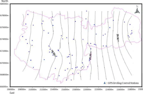
3.1 Research Data and Collection
Figure 2 - The 78 control stations distribution and original geometric undulations contour map of the study area.
3.2 Research Methods
The orthometric height (H) obtained from the spirit leveling information was subtracted from the ellipsoidal height (h) measured using the GPSRTK. The results were used to derive various local geometric geoid undulations (N) to serve as the known values. In this study, Matlab was used asthe LS-SVM calculation platform. The plane coordinates of the points (N, E) were entered in Matlab to calculate the geometric geoid undulation of the fitting region. The results were compared with the known geoid undulation to derive residuals△N. The precision of the local geoid values calculated using various methods were compared with that of the fitting methods used in previous studies(WANG, 2005;CHUNG, 2008; KAO and SHENG, 2011)that used the same experimental condition limits. The various LS-SVM model kernel functions were used to establish the optimal fitting points of the study area. The determined geometric geoid was verified by evaluating the orthometric heights at selected benchmarks. The primary focus of this study was increasing the accuracy of the local geometric geoid, ensuring a simple and rapid transformation of the ellipsoid height into the orthometric height in the test area. Interpolation is a crucial step when determining a local geometric geoid. Substantial computation time may be required if numerous terms of a function are used and a large data set is required to form the model. Surveyors should use the minimum occupied number of GPS and leveling data points to conserve working hours, and the difficult terrain for spirit leveling measurement (e.g., mountainous areas) and ensure the level of accuracy required during practical engineering surveys.
3.3 Research Procedures
The steps of this study are summarized as follows:
(1) Confirm input the plane coordinates of the points (N, E) and output geoid undulation (N).
(2) Select the model parameters and use the polynomial kernel function, using as the third-order polynomial, and using the RBF kernel function grid to select optimal parameters
( ,
γ σ
2)
.In this study,γ
=
5470.122
andσ
2=
34.411
were selected as the parameters.(3) Perform model initialization and use the fit points (training samples) combined with linear, polynomial, and RBF kernel functions to establish the LS-SVM model.
(4) Input the check points (test samples) into the trained LS-SVM model to yield the local geometric geoid undulation forecasts.
4. STUDY RESULTS AND ANALYSIS
methods in the same test area. This comparison was conducted to explore the applicability of the LS-SVM. The same fitting points were tested to compare the accuracy of derived geometric geoid with the results of Wang (2005) and Chung (2008). Therefore 35 of the 78 GPS stations used by WANG (2005) were selected as checkpoints and the remaining 43 stations were used to construct the geometric geoid. The differences between the predicted and known values were used to measure the accuracy of the local geometric geoid. According to the results o Wang (2005), the RMSEs could attain ± 2.00 cm and ± 1.89 cm by adopting curve surface fitting and BP ANNs, respectively, to build the geometric geoid model. According to CHUNG (2008), the RMSEs could attain± 2.62 cm, ± 3.52 cm, and ± 2.62 cm by adopting the hyperbolic curve, 3power of distance, and squared distance methods, respectively. Its precision was sufficient for use in engineering surveys. Therefore in this study, the RMSE was calculated for the same test region and fitting point conditions, using checkpoints that were not employed in model training. The results were used to conduct a comparative analysis. The 43 fitting points and 35 checkpoints used in the BP neural network study of WANG(2005) and the 40 fitting points and 38 check points used in the multi-surface function methods study of(CHUNG,2008) were evaluated. The study area comprised 78 points (fitting points and checkpoints) and Tables 1 and 2 display the relevant results.
Table 1 - Statistics results for35 checkpoint-result geoid undulation differences predicted by three methods for study area.
Method
Second-Order Curve Surface Method(cm) (WANG,2005)
BP Neural Network Method(cm) (WANG,2005)
LS-SVM Method(cm)
RBF Polynomial Linear
N
∆
Max. Value 3.88 -3.60 -3.69 4.62 10.50N
∆
Min. Value -0.12 -0.00 -0.10 0.05 -0.66N
∆
AverageValue 1.66 1.57 1.49 1.55 4.99
N
Table 2 - Statistics results for 38 checkpoint-result geoid undulation differences predicted by three methods for study area.
Method
Multi-Surface Function Method(cm)
(CHUNG,2008) LS-SVM Method(cm)
Hyperbolic Curve
Three Power of Distance
Squared
Distance RBF Polynomial Linear
N
∆
Max. Value 4.66 -9.98 5.27 4.98 -4.96 -16.47N
∆
Mini. Value 0.01 -0.32 0.31 -0.10 0.020 -0.24N
∆
AverageValue 2.25 2.90 2.19 1.89 1.87 4.53
RMSE ±2.62 ±3.53 ±2.62 ±2.34 ±2.34 ±5.79
Because the real geoid surface was modeled as smooth in the test area, any interpolation methods produce similar results (Tables 1 and 2). Thus, the various methods used to derive local geoid model are all suitable and similar. In this study, a method was presented using LS-SVM to approximate the regional geoid surface. Although the fitting performance levels of the various models yield small RMSE differences of a few millimeters, the proposed LS-SVM method yielded the smallest RMSE, indicating that it can refine the approximate geoid surface in the test area. The test results indicated that the accuracy of the estimated geometric undulation interpolation that used the LS-SVM was in the order of 1.5 cm. Based on these results, the estimated undulation accuracy attained using the LS-SVM was superior to that attained using the curve fitting and BPANN methods (LIN, 2007) by an order of 2–4 cm in the same test area.
The results shown in Tables 1 and 2 indicate that although the linear kernel-function calculation results of the geometric geoid undulations derived using the LS-SVM were less precise than were those calculated using the second-order curve surface, BP neural network, and multi-surface function methods, the precision derived using the RBF and polynomial kernel function results was superior to that derived using other methods. Therefore, the LS-SVM was used to calculate local geometric geoid undulations.
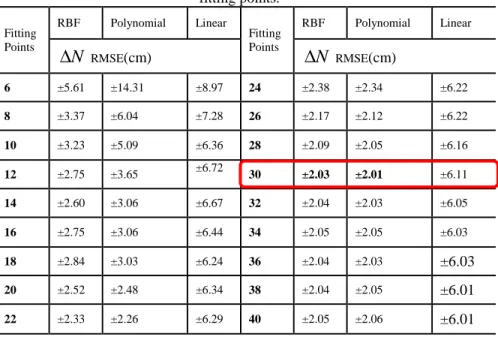
4.1 Optimization Tests
Table 3 - The
∆
N
RMSE results (cm) fitted using various numbers of LS-SVM fitting points.Fitting Points
RBF Polynomial Linear
Fitting Points
RBF Polynomial Linear
N
∆
RMSE(cm)∆
N
RMSE(cm)6 ±5.61 ±14.31 ±8.97 24 ±2.38 ±2.34 ±6.22
8 ±3.37 ±6.04 ±7.28 26 ±2.17 ±2.12 ±6.22
10 ±3.23 ±5.09 ±6.36 28 ±2.09 ±2.05 ±6.16
12 ±2.75 ±3.65 ±6.72 30 ±2.03 ±2.01 ±6.11
14 ±2.60 ±3.06 ±6.67 32 ±2.04 ±2.03 ±6.05
16 ±2.75 ±3.06 ±6.44 34 ±2.05 ±2.05 ±6.03
18 ±2.84 ±3.03 ±6.24 36 ±2.04 ±2.03 ±6.03
20 ±2.52 ±2.48 ±6.34 38 ±2.04 ±2.05 ±6.01
22 ±2.33 ±2.26 ±6.29 40 ±2.05 ±2.06 ±6.01
The results in Table 3 indicate that when the fitting point was at 30, the △N RMSE values derived using the RBF and polynomial methods were minimal and complied with the sample size, which was greater than 30. Errors should be assumed to be normally distributed; therefore, 30 points were used to perform model training and the remaining48 points were used as checkpoints. Figure 4 shows the distributed points.
Figure 4 - Study area fitting-point and checkpoint distribution chart.
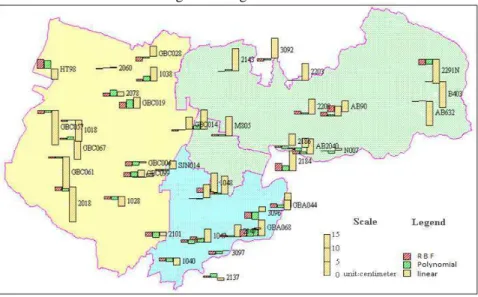
Figure 6 - Differences of local geoid undulation at 48 global positioning satellite-leveling control points for three kernel function of LS-SVM.
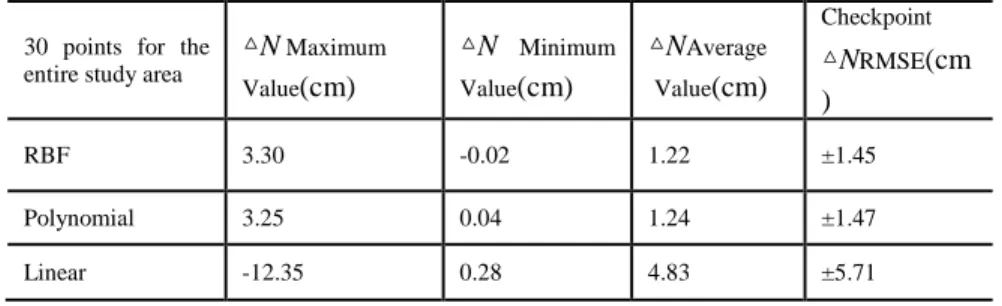
Table 4 - The △N statistic results for the 48-point checkpoint fitting of the study area.
30 points for the entire study area △
N Maximum Value(cm)
△N Minimum Value(cm)
△NAverage Value(cm)
Checkpoint
△NRMSE(cm )
RBF 3.30 -0.02 1.22 ±1.45
Polynomial 3.25 0.04 1.24 ±1.47
Linear -12.35 0.28 4.83 ±5.71
The results shown in Table 4 indicate that the local geometric geoid undulation fitted using the RBF and polynomial kernel functions yielded an overall precision of approximately ±1.47cm compared with that of the known geometric geoid undulation. The results obtained using the linear kernel function exceeded the limitations of indirect elevation observations and inverse elevation calculations, which should be less than 5 cm.
-15 -10 -5 0 5 10
R B F Polynomial linear
Point Name
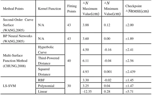
Table 5 - Precision comparison of the local geometric geoid undulation for the test area derived using different fitting methods.
Method Points Kernel Function Fitting Points
△N Maximum Value(cm)
△N Minimum Value(cm)
Checkpoint
△NRMSE(cm)
Second-Order Curve Surface
(WANG,2005)
N/A 43 3.88 0.12 ±2.00
BP Neural Networks
(WANG,2005) N/A 43 3.60 0.00 ±1.89
Multi-Surface Function Method (CHUNG,2008)
Hyperbolic Curve
40
4.50 -0.16 ±2.41
Third-Powered
Distance 6.11 -0.04 ±2.56
Squared
Distance 4.93 0.001 ±2.439
LS-SVM
RBF
30
3.30 -0.02 ±1.45
Polynomial 3.25 0.04 ±1.47
Linear -12.35 0.28 ±5.71
The results presented in Table 5 indicate that compared with the local geometric geoid undulation model of the test area constructed using the second-order curve surface, the BP neural network (WANG, 2005), and multi-surface function methods (CHUNG, 2008), the proposed LS-SVM method requires only 30 fitted points. This is 10 or more points fewer compared with the number required for using the second-order curve surface, BP neural network, or multi-surface function methods; however, the proposed method yields a comparable level of precision.
5.CONCLUSION
In this study, the LS-SVM was applied to construct a local geoid undulation model. Experimental testing indicated that the proposed method effectively predicted geometric geoid undulation and met precision requirements. Various kernel functions can be used to construct distinct LS-SVM models. The results indicated that using RBF and polynomial kernel functions to evaluate the study area produced a superior fitting precision of approximately ± 1.5 cm. The fitting of the linear kernel function was less desirable compared with these methods.
distribution of the known points. In this study, after changing the number of points and point distributions, the 3kernel functions yielded differing fitting results, reducing the number of fitting points by 10 or more. The checkpoint errors of the RBF and polynomial kernel functions were controlled within ± 5 cm, meeting the elevation precision requirements of engineering surveys. This level of precision cannot be achieved using the linear kernel function.
ACKNOWLEDGMENTS
This research was sponsored in part by the National Science Council of Taiwan (Project No. NSC 100-2622-E-005-015-cc3)
REFERENCES
ABDALLA A. et al. The Evaluation of The New Zealand’s Geoid Model Using the KTH Method. Geodesy and Cartography, Vol.37, No.1, p.5-14, 2011.
AKCIN, HAKAN; CELIK, CAHIT TAGI. Performance of Artificial Neural Networks on Kriging Method in Modeling Local Geoid. Boletim de Ciências Geodésicas, Vol.19, No.1, p.84-97,2013.
CHUNG, CHIH-WEI. A Study of Different Multi-surface Functions to Improve the Determined Local Geoid Model-A Case Study of Taichung City. Master thesis. Department of Civil Engineering, National Chung-Hsing University, 2008( in Chinese).
FEATHERSTONE, W. E. et al. Comparison of Remove-Compute-Restore and University of New Brunswick Techniques to Geoid Determination over Australia, and Inclusion of Wiener-Type Filters in Reference Field Contribution. Journal of Surveying Engineering, Vol.130, No.1, ASCE, p.40-47, 2004.
FU,YUAN-YUAN; DONG REN. A Study of Support Vector Machine (SVM) Kemel Function and Parameter Selection, Technology Innovation Herald,Vol.9, p.6-7, 2010 (in Chinese).
HSU, C.W. et al. A Practical Guide to Support Vector Classification. Technical Report, Department of Computer Science and Information Engineering, National Taiwan University, 2003( in Chinese).
KAO, SZU-PYNG; SHEN,YU-TING. A Study of Fitting Local Geoid Model by Least Squares Support Vector Machine─A Case Study of Taichung Area. Joint 30nd Surveying and Geomatics Conference, p.137, 2011( in Chinese).
KAO, SZU-PYNG et al. A study of Using Support Vector Machine (SVM) Method to Determine Local Geoid Model-A Case Study of Taichung Area, Joint 29nd Surveying and Geomatics Conference.p.123, 2010(in Chinese).
KAO, SZU-PYNG;BETHEL, J.S. Geoid from Geopotential Model in the Taiwan Area, Marine Geodesy, Vol.15, No.4, pp.245-252,1992(a).
KAO, SZU-PYNG;BETHEL, J.S. A Study of the Gravimetric Geoid in the Taiwan Area, Presented in the ASPRS-ACSM. Annual Convention, Albuquerque, 1992(b).
LIN,LAO-SHENG. Application of Back-Propagation Artificial Neural Network to Regional Grid-Based Geoid Model Generation Using GPS and Leveling Data. Journal of Surveying Engineering, Vol.133, No.2, ASCE, p.81-89, 2007. SHEN, YU-TING. A Study of Fitting Local Geoid Model by Least Squares Support
Vector Machine-A Case Study of Taichung Area. Master thesis, Department of Civil Engineering, National Chung Hsing University, 2011(in Chinese). SUYKENS,J.A.K.; VANDEWALLE, J. Least Squares Support Vector Machine
classifiers , Neural Processing Letters, Vol.9, No.3, p.293-300,1999.
TRANES, M. D. et al. Comparisons of GPS-Derived Orthometric Heights Using Local Geometric Geoid Models, Journal of Surveying Engineering, Vol.133, No.1, ASCE, p.6-13, 2007.
USTUN, AYDIN, DEMIRE, HUSEYIN. Long-Range Geoid Testing by GPS-Leveling Data in Turkey, Journal of Surveying Engineering, Vol.132, No.1, ASCE, p.15-23, 2006.
VAPNIK,V. N. The Nature of Statistical Learning Theory, New York: Springer-Verlag,1995a.
VAPNIK, V. N. Statistical Learning Theory, New York: John Wiely & Sons, Inc., 1995b.
WANG WEN-AN. A Study of determining regional geoid using different methods ─A Case Study of Taichung City, Thesis , Department of Civil Engineering, National Chung Hsing University, 2005( in Chinese).
YOU, REY-JER. Local Geoid Improvement Using GPS and Leveling Data: Case Study, Journal of Surveying Engineering, Vol.132, No.3, ASCE, p.101-107, 2006.
YANG, ZHAN-JI et al. Determination of Local Geoid with Geometric Method: Case Study, Journal of Surveying Engineering, Vol.125, No.3,ASCE, p.136-146, 1999.
ZHOU QIA. Comparative Study of Support Vector Machine for Several Common Kernel Function and Parameter Selection, Fujian computer,Vol.6, p.42-43, 2009 (in Chinese).