Use of an artificial neural network for
detecting excess deaths due to cholera in
Ceará, Brazil
Maria Lúcia F Penna
Escola Nacional de Saúde Pública. Departamento de Endemias Samuel Pessoa. Rio de Janeiro, RJ, Brasil
Received on 22/10/2002. Reviewed on 28/11/2003. Approved on 19/1/2004. Correspondence to:
Maria Lúcia F Penna
Escola Nacional de Saúde Pública Departamento de Endemias Samuel Pessoa Rua Leopoldo Bulhões, 1480 Térreo 21041-210 Rio de Janeiro, RJ, Brasil E-mail: [email protected]
Keywords
Neural networks (computer). Time series. Forecasting. Cholera, epidemiology. Epidemiologic surveillance.
Abstract
Objective
To evaluate recurrent neural networks as a predictive technique for time-series in the health field.
Methods
The study was carried out during a cholera epidemic which took place in 1993 and 1994 in the state of Ceará, northeastern Brazil, and was based on excess deaths having ‘poorly defined intestinal infections’ as the underlying cause (ICD-9). The monthly number of deaths with due to this cause between 1979 and 1995 in the state of Ceará was obtained from the Ministry of Health’s Mortality Information System (SIM). A network comprising two neurons in the input layer, twelve in the hidden layer, one in the output layer, and one in the memory layer was trained by backpropagation using the fist 150 observations, with 0.01 learning rate and 0.9 momentum. Training was ended after 22,000 epochs. We compare the results with those of a negative binomial regression.
Results
ANN forecasting was adequate. Excessive mortality (number of deaths above the upper limit of the confidence interval) was detected in December 1993 and October/ November 1994. However, negative binomial regression detected excess mortality from March 1992 onwards.
Conclusions
The artificial neural network showed good predictive ability, especially in the initial period, and was able to detect alterations concomitant and a subsequent to the cholera epidemic. However, it was less precise that the binomial regression model, which was more sensitive to abnormal data concomitant with cholera circulation.
INTRODUCTION
The prediction of events in epidemiological surveil-lance is aimed at planning the future needs of Public health and at detecting of disturbances in behavior within a time series, which may indicate an excessive number of cases or deaths. Techniques employed to this end include adjustment to periodic functions, the ARIMA4 models, and Poisson’s regression.1,4,19,16
epide-other neurons. This function is usually a logistic func-tion or a hyperbolic tangent. Such funcfunc-tions are sigmoi-dal in shape, with very little variation for extreme val-ues of x, which simulates the saturation of a biological neuron when incoming stimuli are too intense.
ANNs may be described as a strategy for the math-ematical modeling of problems, which are conceived as systems with inputs and outputs. Unlike in other modeling strategies, one does not need to know the mathematical relationship between inputs and out-puts. Thus, unlike multiple regression, the ANN model does not require a function to be proposed in ad-vance,11 since certain neural networks are capable of approximating any function whatsoever. The network would therefore be able to solve any problem whose relationships it can represent.
Our aim is to evaluate the appropriateness of the use of recurrent neural networks as a predictive tech-nique for time series in Public Health.
METHODS
The study was carried out during a cholera epi-demic which took place in 1993 and 1994 in the state of Ceará, northeastern Brazil, and was based on excess deaths with ‘poorly defined intestinal infec-tions’ as the underlying cause (ICD-9).
Excess mortality was attributed to non-diagnosed lethal cases of cholera.8 Ceará was chosen for having presented, for two consecutive years, the highest yearly incidence rates of cholera ever registered in Brazil – namely 346.19 and 302.74 per 100,000 population, in 1993 and 1994, respectively.
The monthly number of deaths in the state of Ceará between 1979 and 1995 with “poorly-defined intes-tinal infections” (ICD-9) as the underlying cause were obtained from the Ministry of Health’s Mortality In-formation System.
As a comparison we chose negative binomial re-gression, a statistical technique widely employed for this type of data in cases where Poisson regression proves inadequate.15
A recurrent network was built with two neurons in the input layer (corresponding to year and month), twelve in the hidden layer, one in the output layer, and one in the memory layer. The recurrent connection connects the output layer to the memory layer, which, in its turn, is connected to the hidden layer. All activat-ing functions were based on the logistic function. Train-ing was carried out through backpropagation, with 0.01 miological surveillance. When the goal is to detect
excess mortality, longer periods are generally used.
Excess mortality was introduced into epidemio-logical surveillance in the context of evaluating the impact of influenza epidemics.5 This was due to diffi-culties in classifying influenza-related deaths, which were, in their majority, attributed to complications of the infection, such as pneumonia. The concept of excess mortality was also used in evaluating the im-pact of heat waves, atmospheric pollution, and of apparently benign epidemics.
Epidemiological surveillance in Brazil shows greater operational variability than in developed countries, which results in decreased precision (greater variance) of the data and consequently less sensitivity of the notification system in detecting new diseases and the occurrence of epidemics. Thus, the use of excess mor-tality techniques may prove useful for increasing the sensitivity of the surveillance system, since mortality registration has higher coverage and longer available time series than the notification system.
However, the statistical methods traditionally used require profound knowledge of statistics for the se-lection and evaluation of models, which prevents them from being used in a decentralized manner.3,17 Artificial Neural Networks (ANN), on the other hand, have the advantage of being applicable to several time series sequentially, without prior diagnosis of their behavior, providing good results.12,21
In most time series of interest to Public Health, vari-ability is largely attributable to trends and seasonality. Their behavior is non-linear, and their cycles are ir-regular. The advantage of using neural networks to approximate non-linear functions is that this tech-nique has been successful in analyzing series in which the mathematical knowledge of the stochastic proc-ess behind the series is either unknown, or difficult to be rationalized.2
Neural networks were developed initially as a strat-egy for simulating human mental processes – such as image and sound recognition – and later as an effi-cient technological instrument for performing a large number of different tasks.
learning rate and 0.9 momentum. The criterion for train-ing termination was reachtrain-ing 22,000 epochs. NeuroShellâ software was used.23
Data from January 1979 to June 1991 – totaling 150 observations – were used for network training and model adjustment. This choice was aimed at en-suring the absence of Vibrio cholerae circulation in the adjustment period, given that the first case noti-fied in the state of Ceará took place in February 1992, and non-detected cases may have occurred in the immediately preceding months.
Data for the 54-month period between August 1991 and December 1995 were predicted based on the net-work. Due to the change from ICD-9 to ICD-10 in January 1996, we chose not to prolong the extrapola-tion beyond this date in order to ensure the homoge-neity of the series. The confidence interval for the implicit ANN model was estimated based on the dis-tribution of residues from the training period, assum-ing a normal distribution with mean =0. Bootstrapp-ing with 2,000 samples was performed in order to evaluate the adequacy of the parameters directly es-timated from the 150 residues.
Data were also adjusted to a negative binomial dis-tribution, deaths being a function of order of occur-rence, representing month-year, and of month of oc-currence, transformed into a dummy variable, repre-senting the seasonal component, after verifying an over-dispersion in a Poisson regression model. STATA19 soft-ware was used for this analysis.
RESULTS
Table 1 shows the results of negative binomial re-gression. June was removed from the model for colinearity reasons, i.e., according to the adjusted model, June is the baseline month for the definition of the remaining parameters, which express the sea-sonal component. The months between July and No-vember were not statistically significant, but were kept in the model to ensure its validity.
The parameters related to the residues of the neural network are presented in Table 2. The confidence in-tervals around the mean include zero.
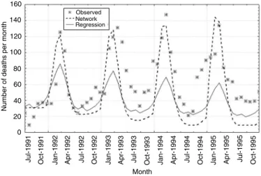
Figure 1 shows estimates from both models for the adjustment period. Agreement between the two mod-els is high, with a 0.95 Pearson correlation coefficient. The mean difference between the two estimates was 0.544740 (95%CI -294971 to 4.039190). Figure 2 presents estimates from both models extrapolated for the July 1991 – December 1995 period. In this case there is less agreement between both estimates, with a 0.92 Pearson correlation coefficient. Mean difference is -6.56195 (95%CI -13.9088 to 0.784901). The esti-mate given by the ANN is higher than that obtained through regression. Although ANN estimates for the December – May period – the season with highest mortality – were closer to the observed values, the val-ues estimated through regression were closer to the observed values in the remaining months.
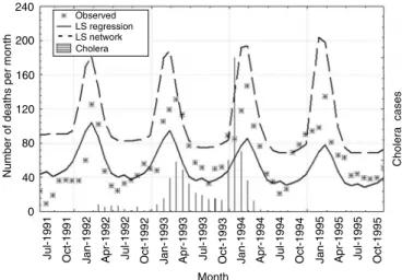
Figure 3 presents the upper limit of the confidence
Table 1 - Results, negative binomial regression: parameters and statistical significance.
Series Coeff. Std. Err. z p>z [95% CI]
Inf. lim. Sup. lim.
Order -0.00893 0.000523 -17.06 0.000 -0.00995 -0.0079
Jan 0.550417 0.10777 5.11 0.000 0.339193 0.761642
Feb 0.788315 0.107209 7.35 0.000 0.578189 0.99844
Mar 0.919921 0.10693 8.6 0.000 0.710342 1.129501
Apr 0.724294 0.107387 6.74 0.000 0.513819 0.934768
May 0.371552 0.108558 3.42 0.001 0.158782 0.584322
July -0.12263 0.112787 -1.09 0.277 -0.34368 0.098431
Aug -0.03607 0.112405 -0.32 0.748 -0.25638 0.184244
Sept -0.18182 0.11329 -1.6 0.109 -0.40387 0.040219
Oct -0.07642 0.112647 -0.68 0.498 -0.2972 0.144366
Nov 0.047475 0.112008 0.42 0.672 -0.17206 0.267007
Dec 0.236944 0.111021 2.13 0.033 0.019347 0.454541
Cons 4.949957 0.087621 56.49 0.000 4.778223 5.121691
Alpha 0.061099 0.008092 0.04713 0.079207
Likelihood ratio test of alpha =0: chibar2(01) =851.78 Prob >= chibar2 =0.000 Number of obs =150 LR chi2(12) =250.16 Prob > chi2 =0.0000
Log likelihood =-690.65416
Table 2 - Parameters estimated from residues of the 150 points used in network training.
Parameter Observed Traditional Bootstrap sample CI estimated by
value parameter CI parameter bootstrapping
Mean 0.57234 -4.3530:5.4976 0.3766 -4.198:5.343
Median -0.67900 -5.048:3.310 — -4.964:3.606
intervals of both estimates, observed data, and cholera occurrence, from July 1991 to December 1995. The regression model detected excess mortality in March-April 1992 – shortly after the detection of the first cases of cholera in the state in February – and in Octo-ber-November 1992. From February 1993 onward, with the exception of August and September 1994, all points were above the upper limit of the regression model. Considering excess mortality as the difference between the number of deaths observed and the upper limit of the confidence interval, the excess mortality – as defined by regression – was 68 deaths in 1992, 266 in 1993, 285 in 1994, and 205 in 1995.
The neural network detected an excess mortality of only five deaths in December 1993, the month pre-ceding the highest peak in the cholera epidemic, and of 17 deaths in November-December 1994, in the fol-lowing season.
DISCUSSION
The results obtained indicate that excess mortality did occur in the state of Ceará in the period, and that it may be possible to detect this excess mortality based on monthly mortality data. In the studied period, 217 deaths due to cholera were registered in the state: 19 in 1992, 89 in 1993, 104 in 1994 and five in 1995. The neural network under-estimated excess mortality. There are doubts concerning the considerable magnitude of the binomial regression estimate for 1995. Such magnitude may be due to the extended extrapolation period. Prolonging the series to encompass the period immediately follow-ing would perhaps clear this point. Unfortu-nately, the change from ICD-9 to ICD-10 would cast doubts on the homogeneity of
the series, introducing a likely bias and ham-pering result interpretation.
It should be noted that, with respect to the season with the greatest number of deaths as-cribed to poorly defined intestinal infections, point estimates provided by the neural network were closer to the observed values than those provided by negative binomial regression in the extrapolation period (Figure 2), but not in the model-adjustment period (Figure 1), sug-gesting that, for longer intervals, extrapolation through binomial regression is less reliable than that provided by neural networks. This poten-tial characteristic of the neural network, how-ever, is not advantageous, since interval esti-mation has low levels of precision.
Estimates from both models showed good agree-ment, indicating the adequacy of using ANNs for health-related time series. However, from a more prag-matic standpoint – the usual approach in economet-rics – the choice between different prediction strate-gies must tend towards that which correctly predicts the outcome. In epidemiological surveillance, the subject of the prediction is the detection of abnormal values20 rather than the greater proximity between predicted and observed numbers – which is the case with price prediction, for instance. In the present case, negative binomial regression was more adequate for the detection of excess deaths during the circulation of Vibrio cholerae due to its narrower variance.
The difference between negative binomial regres-sion and Poisson regresregres-sion resides in its estimation of variance, which incorporates an over-dispersion parameter – alpha. This method was used only be-cause residues registered after adjustment of a
Figure 1 - Observed and estimated mortality: negative binomial regression and neural network. January 1979 to June 1991.
400
350
300
250
200
150
100
50
0
May-79 Feb-82 Nov-84 Aug-87 May-90
Month
Number of deaths per month
Observed Network Regression
Figure 2 - Mortality observed and estimated by extrapolation: negative Binomial regression and neural network. July 1991 to December 1995.
160
140
120
100
80
60
40
20
0
Month
Jul-1991 Oct-1991 Jan-1992 Apr-1992 Jul-1992 Oct-1992 Jan-1993
Number of deaths per month
Observed Network Regression
Poisson regression showed greater dispersion than their corresponding distributions. When alpha equals zero, negative binomial distribution is reduced to Poisson distribution.
Different strategies have been used for error esti-mation in neural network predictions.2 The one used in the present study is based on the assumption that, theoretically, an exact model for the time series can be found, but that, due to measurement errors and to the influence of uncontrollable and unknown factors, there is a randomly produced residual error, and the neural network is a quasi-optimal model. This is doubt-less an area to be further explored and developed.
The neural networks most used are the non-recur-rent or feed-forward networks. In this model each neu-ron in a given layer interacts with al neuneu-rons in adja-cent layers, but not with those in the same layer, processing occurring always in one direction, from input to output. By contrast, recurrent neural net-works, such as the one employed in the present study, are capable of learning sequences and are thus the best choice for dealing with time-series data. Whereas networks with standard connections respond to a given input always through the same output, a recur-rent network can respond to a same input through different outputs at different moments, depending on the input previously presented.
When incorporating a neuron into the memory layer, the network is incorporating an auto-regressive com-ponent,22 in addition to the trend and seasonality com-ponents represented by the two input neurons, year and month. The auto-regressive component allows the values predicted at a given moment to influence the subsequent prediction, ascribing greater influence to
recent values. This did not generate diver-gence between models, despite the negative binomial regression not considering auto-cor-relation in time.
The main difficulty faced in using neural networks is that, due to the novelty of the method, researchers in general have little familiarity with the process, compared to other statistical methods.14 The criterion for choosing between different networks is pragmatic, i.e., the network chosen is that which fulfils the objectives expected. Re-sult reproducibility is also not guaranteed, since initial weights are random in each training session – which may lead to differ-ent areas in the error surface –, and since there are different convergence criteria – which may result in different local minimums. These characteristics contribute towards a certain degree of uncertainty in using this instrument, which can be overcome by carrying out several training ses-sions and observing result distribution.
Another problem mentioned in the literature9 is over-training, by which the network captures quantitative relationships generated by noise from the data, with negative effects on generalization (external validity). An alternative is to compare networks with different training times.6,7 The network presented in the present study was the first one adjusted, no important differ-ences having been detected in subsequent networks. One may say that the criterion for convergence was learn-ing ‘time’, since convergence was determined by the number of times the entire set of data was presented during training. The ‘training set’ comprised the data from the period preceding the introduction of cholera in the country. A separate calibration set was not deter-mined, since the size of the training set has important implications on generalization. In this case, the calibra-tion method – cross-validacalibra-tion – would not compensate for the reduction in the size of the training set.
In this example, the neural network was less sensitive than negative binomial regression. Its main advantage was the lower level of statistical knowledge required for its application. It was clearly the technique most easily applicable in the present example, since it did not im-ply the recognition of models according to the behavior of the series, nor the evaluation of the adjusted model. The present results indicate promising aspects in the use of neural networks in epidemiological surveillance. However, there is still need for deepening theoretical knowledge of the statistical behavior of network residues, so as to allow for greater estimate precision.
Figure 3 - Upper limit of the confidence interval, estimated through negative binomial regression and neural network. July 1991 to December 1995.
240
200
160
120
80
40
0
Number of deaths per month
Month
Cholera cases
Observed LS regression LS network Cholera
REFERENCES
1. Alves MT, Silva AAM, Nemes MIB, Brito GO. Tendência da incidência e da mortalidade por Aids no Maranhão, 1985 a 1998. Rev Saúde Pública
2003;37:177-82.
2. Castiglione F. Forecasting price increments using an artificial neural network. Adv Complex Systems
2001;4:45-56.
3. Chatfield C. The analysis of time series. 4th ed. London: Chapman & Hall; 1994.
4. Choi K, Thacher SB. An evaluation of influenza mortality surveillance, 1962-1979. Am J Epidemiol
1981;113:215-22.
5. Collins SD, Lehman J. Trends and epiemics of influenza and penumonia, 1918-1951. Public Heath Rep 1951;66:1487-505.
6. Duh M, Walker AM, Pagano M, Kronlund K. Prediction and cross-validation of neural networks versus logistic regression: using hepatic disorders as an example. Am J Epidemiol 1998;147:407-12.
7. Duh M, Walker AM, Ayanian JZ. Epidemiologic interpretation of artificial neural networks. Am J
Epidemiol 1998;147:1112-9.
8. Gerolomo M. Cólera no Brasil:a sétima pandemia [tese de doutorado]. Rio de Janeiro: Instituto de Medicina Social da UERJ; 2002.
9. Gorni AA. The application of neural networks in the modeling of plate rolling processes. JOM-e [serial on-line] 1997; 49. Available from: URL:http://
www.tms.org/pubs/journals/JOM/9704/Gorni/Gorni-9704.html [2003 nov 12]
10. Haykins S. Neural Networks, a comprehensive foundation. 2nd ed. New Jersey: Prendice Hall; 1999.
11. Haydon GH, Jalan R, Ala-Korpela M, Hiltunen Y, Hanley J, Jarvis LM, Ludlum CA, Hayes PC. Prediction of cirrhosis in patients with chronic hepatitis C infection by artificial neural network analysis of virus and clinical factors. J Viral Hepat 1998;5:255-64.
12. Joo CN, Koo JY, Yu MJ. Application of short-term water demand prediction model to Seoul. J Water Sci
Technol 2002;46:255-61.
13. Kao JJ, Huang SS. Forecasts using neural network versus Box-Jenkins methodology for ambient air quality monitoring data. J Air Waste Manag Assoc
2000;50:219-26.
14. Kattan MW, Hess KR, Beck JR. Experiments to determine whether recursive partitioning (CART) or an artificial neural network overcomes theoretical limitations of Cox proportional hazards regression.
Comput Biomed Res 1998;31:363-73.
15. Lawless JF. Negative binomial and mixed Poisson regression. Can J Stat 1987;15:209-25.
16. Simonsen L, Clark MJ, Stroup DF, Williamson GD, Arden NH, Cox NJ. A method for timely assessment of inflenza associated mortality in the United States.
Epidemiology 1977;8:390-5.
17. StatSoft Inc. STATISTICA for Windows [Computer program manual]. Tulsa; 1998.
18. Stroup D, Wharton M, Kafadar K, Dean AG. Evaluation of a method for detecting aberrations in public health surveillance data. Am J Epidemiol
1993;137:373-80.
19. StataCorp. Stata statistical software: release 7.0. College Station, TX; 2000.
20. Teush SM, Churchill RE. Principles and practice of
public health surveillance. New York: Oxford
University Press; 1994.
21. Tu JV. Advantages and disadvantages of using artificial neural networks versus logistic regression for predicting medical outcomes. J Clin Epidemiol
1996;49:1225-31.
22. Wasserman PD. Neural computing: theory and practice. New York: Van Nostrand Reinhold; 1989.