www.atmos-chem-phys.net/10/11277/2010/ doi:10.5194/acp-10-11277-2010
© Author(s) 2010. CC Attribution 3.0 License.
Chemistry
and Physics
Multi sensor reanalysis of total ozone
R. J. van der A, M. A. F. Allaart, and H. J. Eskes
KNMI, P.O. Box 201, 3730 AE De Bilt, The Netherlands
Received: 23 February 2010 – Published in Atmos. Chem. Phys. Discuss.: 28 April 2010 Revised: 12 August 2010 – Accepted: 16 November 2010 – Published: 30 November 2010
Abstract. A single coherent total ozone dataset, called
the Multi Sensor Reanalysis (MSR), has been created from all available ozone column data measured by polar orbit-ing satellites in the near-ultraviolet Huggins band in the last thirty years. Fourteen total ozone satellite retrieval datasets from the instruments TOMS (on the satellites Nimbus-7 and Earth Probe), SBUV (Nimbus-7, NOAA-9, NOAA-11 and NOAA-16), GOME (ERS-2), SCIAMACHY (Envisat), OMI (EOS-Aura), and GOME-2 (Metop-A) have been used in the MSR. As first step a bias correction scheme is applied to all satellite observations, based on independent ground-based total ozone data from the World Ozone and Ultravio-let Data Center. The correction is a function of solar zenith angle, viewing angle, time (trend), and effective ozone tem-perature. As second step data assimilation was applied to create a global dataset of total ozone analyses. The data assimilation method is a sub-optimal implementation of the Kalman filter technique, and is based on a chemical transport model driven by ECMWF meteorological fields. The chemi-cal transport model provides a detailed description of (strato-spheric) transport and uses parameterisations for gas-phase and ozone hole chemistry. The MSR dataset results from a 30-year data assimilation run with the 14 corrected satel-lite datasets as input, and is available on a grid of 1×11/2◦
with a sample frequency of 6 h for the complete time pe-riod (1978–2008). The Observation-minus-Analysis (OmA) statistics show that the bias of the MSR analyses is less than 1% with an RMS standard deviation of about 2% as com-pared to the corrected satellite observations used.
Correspondence to:R. J. van der A ([email protected])
1 Introduction
Although ozone observations from space are available for 1971 and 1972 with the BUV instrument on Nimbus-4 (Sto-larski et al., 1997), regular and continuous ozone monitor-ing from space in the UV-VIS spectral range is performed since 1978 with the TOMS and SBUV instruments on the satellite Nimbus-7 (Bhartia et al., 2002; Miller et al., 2002). These observations were continued with the TOMS instru-ments on Meteor 3, Earth Probe, and ADEOS until the year 2003, when the measurements started to be seriously af-fected by instrument degradation. This TOMS time series was interrupted from May 1993 until July 1996 when TOMS-EP was launched. However, this gap was filled by contin-uous SBUV observations on various NOAA satellite mis-sions. The gap was also partly filled with GOME ozone observations since July 1995 aboard ERS-2 (Burrows et al., 1999), the first European satellite instrument measuring to-tal ozone from the UV-VIS. Although global coverage was no longer possible due to an instrumental problem in 2003, the GOME instrument is still measuring with reduced cov-erage. Follow-up European satellite instruments are SCIA-MACHY (Bovensmann et al., 1999) launched in 2002 on the Envisat platform of European Space Agency (ESA) and OMI (Levelt et al., 2006), a Dutch-Finnish instrument on the EOS-AURA platform of National Aeronautics and Space Admin-istration (NASA), launched in 2004. The UV-VIS spectrom-eter GOME-2 (Callies et al., 2000) was launched in 2006 on the first of a series of three operational EUMETSAT Metop missions, which allows continuous monitoring of the ozone layer until about 2020.
This study covers a period of more than 30 years of total ozone measurements from space using several UV-VIS satel-lite instruments. These datasets covering a long time period are important for monitoring stratospheric ozone, trend anal-yses (e.g. Stolarski et al., 1991; Fioletov et al., 2002, Brunner et al., 2006a; Stolarski et al., 2006b; WMO, 2007; M¨ader et al., 2007; Harris et al., 2008) and calculating the UV radi-ation at the Earth’s surface (Lindfors et al., 2009; Krcy´scin, 2008). However, the measurements used are originating from different instruments, different retrieval algorithms and are suffering from instrument problems like radiation damage. The data usually shows offsets in overlapping time periods and differ from ground observations. A consistent long-term ozone dataset is important for quantifying ozone de-pletion and detecting first signs of recovery (e.g. Reinsel et al., 2005), following actions to reduce ozone-depleting sub-stances as regulated by the Montreal Protocol and its amend-ments. In 1996, McPeters and Labow published a 14-year ozone dataset based on TOMS measurements and consistent with 30 Dobson and Brewer stations. Bodeker et al. (2001) constructed a 20 year ozone time series based on 5 homoge-nized satellite datasets using ground data as reference, which was later updated using data assimilation (Bodeker et al., 2005) and used to derive the vertical ozone distribution using data assimilation (Brunner et al., 2006b). Recently, Stolarski et al. (2006a) have created a dataset from 1978–2006 by com-bining TOMS and SBUV data. An overview of ozone trend studies before 2006 is provided in the WMO assessment of 2006 (WMO, 2007; and references therein).
The assimilation of ozone measurements has received con-siderable attention in the past 12 years. With the extension to the stratosphere, numerical weather prediction models have also included ozone as explicit model variable (Derber and Wu, 1998). The 40-year reanalysis of the European Cen-tre for Medium-Range Forecasts (ECMWF) includes the as-similation of ozone column satellite data (Dethof and H´olm, 2004) and is one of the first long-term ozone records avail-able based on assimilated satellite data. This work high-lighted some of the difficulties in generating a consistent data set based on a changing observation system and issues that may arise when only total column ozone data is available. Several other centres have set up near-real time and reanal-ysis capabilities to analyse ozone column data from satel-lites (e.g. Geer et al., 2006; Stajner et al., 2008; Eskes et al., 2003). Recently, Kiesewetter et al. (2010) presented a long-term stratospheric ozone data set from the assimilation of SBUV data.
In this paper we present a continuous and consistent ozone column dataset of 30 years, based on the assimilation of satellite observations. The data assimilation method (Eskes et al., 2003) is based on the Kalman filter technique that ex-pects unbiased input data with a known Gaussian error distri-bution. In order to provide these unbiased input data, first a new retrieval (level 2) dataset has been created by correcting all satellite data for biases using ground data as a reference.
(Level 2 data is defined as “geolocated geophysical product”; in this paper it is the retrieved ozone column on the satellite footprint.) These datasets are corrected for biases as func-tion of the solar zenith angle, viewing angle, time (trend), and effective ozone temperature, which are critical parame-ters for errors in the retrievals. Sometimes two level 2 data sets from the same instrument are available. However, these data sets from the same instrument can be seen as indepen-dent measurements since their errors are not more correlated than the errors within a single data set. In order not to show any preferences, both data sets have been used.
Fourteen total ozone satellite datasets have been identified and collected from the satellite instruments TOMS, SBUV, GOME, SCIAMACHY, OMI and GOME-2. In addition, all ground based total ozone observations have been col-lected from the World Ozone and Ultraviolet Data Center (WOUDC, 2009) archive, and a dataset with global effec-tive ozone temperatures has been created. These datasets are described in Sect. 2. A reference dataset has been selected, and the corrections that need to be applied to the satellite datasets to bring them in line with the reference dataset have been computed. These corrections are described in Sect. 3. An intermediate dataset, called the Multi Sensor Reanaly-sis (MSR) level 2 dataset, has been created. This dataset contains virtually all corrected satellite measurements for the thirty-year period. The data assimilation system (TM3-DAM) has been modified slightly to make the best use of the data. This modification is described in Sect. 4. In Sect. 5 the final MSR level 4 data, created with the data assimilation system, is analyzed.
2 Ozone observations
2.1 Satellite ozone measurements
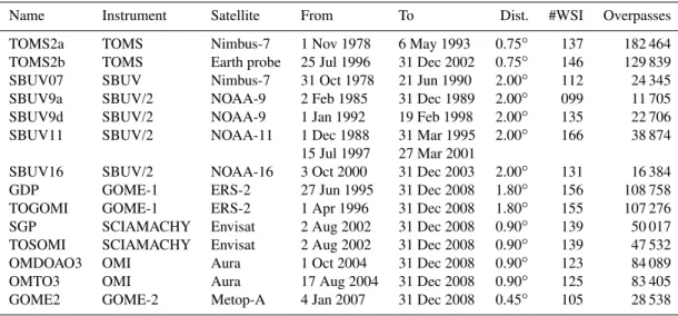
The fourteen satellite total ozone datasets used in this study are listed in Table 1. Each dataset is identified with an acronym: TOMS2a, TOMS2b, SBUV07, SBUV9a, SBUV9d, SBUV11, SBUV16, GDP, TOGOMI, SGP, TO-SOMI, OMDOAO3, OMTO3, and GOME2. Details on the datasets are presented in Appendix A. Two other datasets have been used in this study, namely the WOUDC collection of ground based total ozone data (Sect. 2.2), and a dataset of ECMWF effective ozone temperatures (Sect. 2.5).
Table 1.The satellite datasets used in this study. The columns show the name of the dataset, the satellite instrument on which it is based, the satellite, the period(s) used, the maximum distance allowed in an overpass, the number of ground instruments (WSI) and the total number of overpasses for this dataset.
Name Instrument Satellite From To Dist. #WSI Overpasses
TOMS2a TOMS Nimbus-7 1 Nov 1978 6 May 1993 0.75◦ 137 182 464
TOMS2b TOMS Earth probe 25 Jul 1996 31 Dec 2002 0.75◦ 146 129 839
SBUV07 SBUV Nimbus-7 31 Oct 1978 21 Jun 1990 2.00◦ 112 24 345
SBUV9a SBUV/2 NOAA-9 2 Feb 1985 31 Dec 1989 2.00◦ 099 11 705
SBUV9d SBUV/2 NOAA-9 1 Jan 1992 19 Feb 1998 2.00◦ 135 22 706
SBUV11 SBUV/2 NOAA-11 1 Dec 1988 31 Mar 1995 2.00◦ 166 38 874
15 Jul 1997 27 Mar 2001
SBUV16 SBUV/2 NOAA-16 3 Oct 2000 31 Dec 2003 2.00◦ 131 16 384
GDP GOME-1 ERS-2 27 Jun 1995 31 Dec 2008 1.80◦ 156 108 758
TOGOMI GOME-1 ERS-2 1 Apr 1996 31 Dec 2008 1.80◦ 155 107 276
SGP SCIAMACHY Envisat 2 Aug 2002 31 Dec 2008 0.90◦ 139 50 017
TOSOMI SCIAMACHY Envisat 2 Aug 2002 31 Dec 2008 0.90◦ 139 47 532
OMDOAO3 OMI Aura 1 Oct 2004 31 Dec 2008 0.90◦ 123 84 089
OMTO3 OMI Aura 17 Aug 2004 31 Dec 2008 0.90◦ 125 83 405
GOME2 GOME-2 Metop-A 4 Jan 2007 31 Dec 2008 0.45◦ 105 28 538
2.2 Ground based data
At many sites across the globe ground based instruments are employed to measure total ozone on a daily basis. This long-term dataset provides an excellent reference for the valida-tion of satellite instruments. Extensive research in the perfor-mance of this network has been recently published by Fiole-tov et al. (2008). Their Table 3 shows the characteristics of the different components of the network. The WOUDC col-lects these ground-based observations, and makes them avail-able for research. From this collection a WOUDC-Station-Instrument (WSI) list has been defined. This list has an entry for each type of instrument for each ground station, where type of instrument refers to Dobson (113), Brewer MKII (40), Brewer MKIII (14), Brewer MKIV (39), Filter (62), and Other (7). The number between brackets is the total number of each instrument occurring in the WSI list. In total the WSI-list contains 275 instruments. A discussion of the dif-ferences between the various ground instruments is beyond the scope op this paper. Some information is available in Staehelin et al. (2003).
The daily average total ozone observations for each WSI, in the period 1978–2008, have been extracted. The time re-solved observations have not been used, as these are available only for a limited number of stations. All ground instruments distinguish between DirectSun and ZenithSky observations. DirectSun data is deemed superior, as the retrieval is rela-tively straightforward, not requiring the calculation (explic-itly or implic(explic-itly) of light scattered in the atmosphere. For some of the Brewer sites the ZenithSky data appears not to have been calibrated properly (Fioletov et al., 2008). There-fore, only DirectSun data have been used in this study.
Data that seems odd (for example Direct Sun observations during the polar night) have been rejected. Furthermore a “blacklist” has been created that indicates for each year and for each WSI if the data is suspect. Suspect data has been identified by comparison with various satellite datasets. If sudden jumps, strong trends or very large offsets are identi-fied, the WSI is blacklisted. This subjective blacklist is quite similar to the one used by Bodeker et al. (2001). In total 5% of the ground data has been blacklisted.
2.3 Satellite overpass datasets
of the footprint to the ground station. There can be up to fifteen overpass values per day. From these only one is se-lected and used. This is the one with the smallest reported observation error or the one closest to the ground station if the observation error is not available.
2.4 Seasonal behaviour
With the WOUDC observations and the satellite overpass data prepared as discussed above, it is now possible to com-pare these measurements for each WSI. As an example Fig. 1 shows the monthly averaged anomalies (defined as satellite measurement minus ground measurement) over the Nether-lands as a function of time. It is clear that either the ground station data and/or the satellite data contain a seasonally de-pendent error. A study of all satellite products for this sta-tion (Brewer MKIII, De Bilt) shows that a seasonal effect like this is fairly typical, but the amplitude and phase dif-fers from one satellite product to the other. The seasonal cy-cles of the anomaly of the two satellite products shown here are even in anti-phase. This suggests that at least some of the satellite products have a seasonal offset. A study of all European ground stations versus one satellite product shows that for a large majority of ground stations the results are similar. One cannot conclude from this that the data from the ground stations is essentially correct, as the ground sta-tions are normally calibrated by inter-comparison. Further inspection shows, however, that the seasonal offsets between ground stations and satellite products are clearly different in other regions of the world. This suggests that the offset could depend on latitude, SZA and/or effective ozone temperature, rather than time. It is not uncommon to find seasonal anoma-lies when satellite ozone values are compared to other ozone products, see for example Lerot et al. (2009), Bodeker et al. (2001) and Eskes et al. (2005).
2.5 Effective ozone temperature
The ozone absorption cross-section needed as input for the retrieval algorithms depends on temperature. Ignoring this effect will lead to a time and certainly seasonal depen-dent offset in the total ozone data. This is true for both ground stations and satellite products. A dataset of effective ozone temperatures has been created to study the tempera-ture dependence of the total ozone data. The effective ozone temperature is defined as the integral over altitude of the ozone profile-weighted temperature. This dataset was cal-culated from ECMWF (6 hourly) temperature profiles, and the (seasonal dependent) Fortuin and Kelder ozone climatol-ogy (Fortuin and Kelder, 1998). For the years 1978–1999 the ECMWF ERA40 reanalyses, and for the years 2000–2008, the ECMWF operational analyses have been used. For each ground station a dataset of daily values was created with the effective ozone temperatures interpolated to local noon.
Fig. 1. Monthly averaged anomalies for the overpass data at the ground station De Bilt (5.18◦E, 52.1◦N) in the Netherlands. The anomalies for TOMS2b (red) correlate with effective ozone temper-ature, while the anomalies for TOSOMI (green) correlate with solar zenith angle.
2.6 The reference dataset
Creating a consistent and coherent assimilated dataset re-quires that systematic offsets between the satellite retrieval products are small. A practical way to accomplish this is to choose a reference dataset, and subsequently correct the systematic effects in the other datasets, to bring them in line with the reference dataset. As the true total ozone values are not known, the choice of a reference dataset is somewhat arbitrary. The ground measurements are a logical choice, because these are present for the full 30-year period. The DirectSun measurements from the ground stations are a prime candidate. However, the measurement method used by the Brewer instruments is very sensitive to small details in the ozone absorption cross section, and the various avail-able laboratory measurements of the ozone absorption co-efficients give totally different dependencies of the retrieved total ozone values as function of the effective ozone tempera-ture (Redondas and Cede, 2006). Kerr (2002) has developed a new methodology for deriving total ozone and effective ozone temperature values from the observations made with a Brewer instrument. He concludes that the effective ozone temperature has little effect on the amount of ozone derived with the standard algorithm. So in this study the data from the Brewer network has been adopted as a primary reference. There are 21 stations in the WOUDC database where a Dobson instrument is co-located with a Brewer instrument. This, together with the effective ozone temperatureTeff (in
Xcorr=Xdobson·(1−0.0013·(Teff+46.3)) (1)
has been applied to all Dobson total ozone data.
The WOUDC database contains data from 62 Filter in-struments. These instruments are typically located in for-mer USSR countries. Insufficient Filter instruments are co-located with either Brewer or Dobson instruments to make a statistical analysis of the behaviour of this instrument. A sta-tistical analysis of ground station minus satellite total ozone values for these instruments has shown that the random mea-surement errors (or “noise”) of these instruments are signif-icantly higher than those of the Brewer or Dobson Instru-ments. Therefore the Filter instruments have not been used in the reference dataset.
In summary, the reference dataset consists of all WOUDC instruments, excluding the Filter instruments, and the Dob-son data has been corrected for effective ozone temperature.
3 Corrections for the satellite datasets
3.1 Introduction
In this section the procedure to calculate corrections to the various satellite total ozone datasets will be presented. Ozone differences are defined as: “ground based observations mi-nus satellite observations”. The corrections are obtained by fitting these differences as a function of “predictors” using a simple multi-dimensional least squares fitting system. The predictors are the auxiliary information available in the satel-lite product, and the effective ozone temperature (Sect. 2.5). The fitting procedure uses all overpasses shown in Table 1 to calculate the corrections for the satellite dataset in question.
3.2 Choice of the predictors
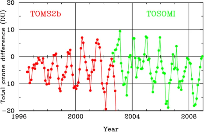
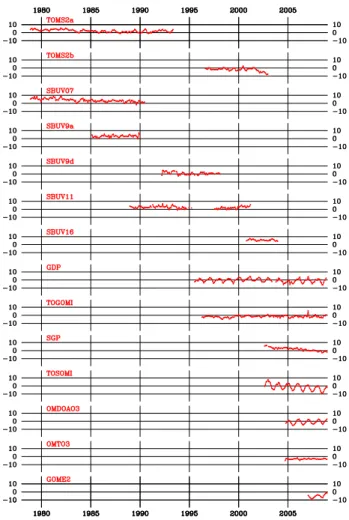
The ozone differences (satellite minus ground observation) show a clear seasonal cycle, which is illustrated in Fig. 2a, where the satellite observations are compared with ground observations. This led to the choice of SZA and effective ozone temperature as predictors, as these imply a clear sea-sonal component. Note that it has been checked that the SZA and effective ozone temperature are not interchangeable as predictor. Some of the satellite products show a clear trend in time, so the number of years since 2000 is another obvi-ous choice. The scan- or view angle is also used as predic-tor. Although most satellite datasets contain this quantity, it is defined in various ways. To overcome these differences, the Viewing Zenith Angle (VZA) has been defined as the an-gle in the scanning direction (or increasing row number for OMI), with the largest negative value in the beginning of the scan, zero at nadir, and the largest positive angle at the end of the scan. It was found that some of the data product anoma-lies have a non linear dependence on VZA. In these cases an offset per pixel along the “scan” was used.
Fig. 2a. Monthly averaged and globally averaged difference of the satellite ozone observation minus the ground observation in units of DU, for all satellite data sets used as function of time.
Bodeker et al. (2001) analyzed ozone differences in terms of time and latitude only. They have used 22 predictors for their fit. The approach in this paper is different, because SZA and effective ozone temperature appeared to be better predictors. Furthermore, these are critical parameters in the retrieval schemes and therefore constitute a more satisfying choice to estimate systematic biases. When these predictors are used the need for an explicit seasonal or latitudinal de-pendence almost disappears. A WSI dependent offset was al-lowed when the regression coefficients were computed. This has been done to reduce the effect (e.g. spurious trends) of “appearing” and “disappearing” ground stations during the lifetime of the satellite instrument from the results.
A basic assumption is that all the corrections are additive to the total ozone amount: Xcorr=Xsat+P
i
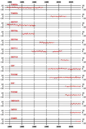
Fig. 2b.Monthly averaged and globally averaged difference of the corrected (as described in Sect. 3.5) satellite ozone observation mi-nus the ground observation in units of DU, for all satellite data sets used as function of time.
3.3 Calculation of the corrections
The regression coefficients for the four predictors and for all fourteen satellite datasets are listed in Table 2. As indicated in Sect. 3.2, an additional offset per WSI (one offset for each type of instrument at each ground station) was used, which are not shown in Table 2. Thus, the total number of predic-tors is in the order of 150 per satellite dataset. Note that the SBUV instruments perform only nadir measurements and the VZA dependence is therefore absent.
Clearly visible are the trends in the SCIAMACHY and GOME2 datasets. For four datasets (TOMS2b, GDP, TO-GOMI, and GOME-2) the VZA dependence is not linear, so the value given here is only indicative. The same is true for the SZA value in the OMDOAO3 dataset. The tempera-ture dependence varies from−0.44 to+0.34 DU/K. The two OMI products show opposite temperature dependency, e.g. negative for OMTO3 and positive for OMDOAO3.
For the purpose of data assimilation it is relevant to re-duce offsets, trends and long-term variations in the satellite data, so that the data can be used as input to the assimila-tion scheme without biases and with known standard devia-tions. The satellite data set corrections are based on a few relevant regression coefficients fitted for the overpass time series of all stations together. By fitting all data together regional biases that may be caused by offsets of individual ground instruments are avoided. From here on the offset per WSI reported above will no longer be used. The relevant re-gression coefficients, i.e. those that reduce the RMS (Root Mean Square) between satellite and ground observations sig-nificantly, have been calculated and are shown in Table 3. Note that in this paper all RMS values have been calculated with the mean value of the data as reference, thus a correc-tion of the overall offset will not improve the RMS. The total RMS is in fact dominated by the error of the ground obser-vations, the representativity errors and the variance of the observations which are larger than the bias terms. A small decrease of the RMS is expected as a result of the correction. The details of the resulting corrections are detailed in Ap-pendix A. The TOMS2b dataset has been corrected for a trend for the last two years only. The datasets that show a non-linear dependence on VZA have been corrected on a “per pixel” basis. There could however be an issue with cor-recting on a “per pixel” basis. If the satellite is in an orbit with a short repeat cycle, each pixel gets calibrated with a unique subset of ground stations. This could lead to a spu-rious offset per pixel. Selecting an orbit with a long repeat cycle should avoid this issue in future missions. The OM-DOAO3 dataset has been corrected for a quadratic SZA de-pendence (indicated with “nonlin” in Table 3).
Table 2. Regression coefficients (expressed as corrections) for the various ozone datasets. The columns are (1) Name; (2) RMS original data; (3) Trend correction; (4) Viewing zenith angle correction, (5) Solar zenith angle correction; (6) Effective ozone temperature correction; (7) RMS after application of these corrections.
Name RMS1 Trend VZA SZA Teff RMS2
(DU) (DU/year) (DU/deg.) (DU/deg.) (DU/C◦) (DU)
TOMS2a 8.97 0.05 0.01 0.01 −0.43 8.75
TOMS2b 8.98 0.51 0.02 0.02 −0.43 8.61
SBUV07 10.01 0.29 N/A −0.03 −0.19 9.95
SBUV9a 10.43 −0.95 N/A 0.11 −0.16 10.28
SBUV9d 9.68 −0.03 N/A −0.04 −0.26 9.63
SBUV11 9.89 0.05 N/A 0.06 −0.17 9.79
SBUV16 9.61 0.31 N/A 0.01 −0.44 9.33
GDP 8.89 0.00 0.05 −0.11 0.03 8.72
TOGOMI 8.08 −0.17 0.07 0.01 −0.01 7.94
SGP 9.11 1.09 −0.01 −0.04 -0.07 8.92
TOSOMI 8.66 1.04 0.05 −0.27 0.05 7.67
OMDOAO3 8.55 −0.36 −0.01 −0.07 0.34 8.19
OMTO3 6.62 0.13 −0.05 −0.05 −0.39 6.46
GOME2 7.21 −2.19 −0.03 −0.19 −0.10 6.60
(MSR-L2) 8.77 0.00 0.00 0.02 0.03 8.76
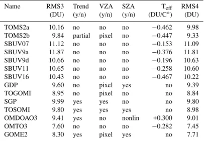
Table 3. Corrections that have been applied to the satellite datasets. The columns are: (1) Name; (2) RMS original data; (3) Trend correction; (4) View angle correction; (5) Solar angle correction; (6) Effective ozone temperature correction; (7) RMS after application of these corrections. Only one offset per satellite instrument is used here.
Name RMS3 Trend VZA SZA Teff RMS4
(DU) (y/n) (y/n) (y/n) (DU/C◦) (DU)
TOMS2a 10.16 no no no −0.462 9.98
TOMS2b 9.84 partial pixel no −0.447 9.33
SBUV07 11.12 no no no −0.153 11.09
SBUV9a 11.87 no no no −0.376 11.81
SBUV9d 10.66 no no no −0.196 10.63
SBUV11 10.65 no no no −0.258 10.60
SBUV16 10.43 no no no −0.467 10.22
GDP 9.60 no pixel yes no 9.39
TOGOMI 8.95 no pixel no no 8.84
SGP 9.99 yes yes no no 9.80
TOSOMI 9.80 yes yes yes no 8.98
OMDOAO3 9.41 yes no nonlin +0.300 9.01
OMTO3 7.60 no no no −0.282 7.45
GOME2 8.30 yes pixel yes no 7.71
spurious trend in the ozone data, if the satellite products are not corrected for effective ozone temperature.
3.4 Random errors
The data assimilation procedure requires a noise estimate for each observation. Not all datasets, however, provide a mea-surement error, and it is unclear if the meamea-surement errors of one product can be compared to those in other products.
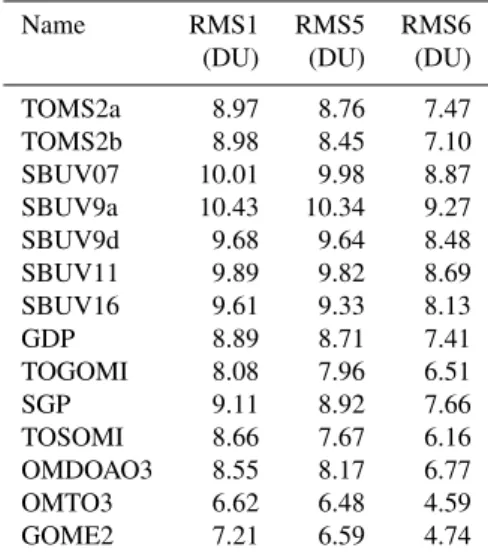
will be shown that the noise in the Brewer and the Dobson datasets are indeed similar.) For all satellite datasets the RMS of the ozone anomalies is computed, allowing for an offset per WSI. These values are shown as “RMS1” (before correc-tions) and “RMS5” (after correccorrec-tions) in Table 4. Assuming the errors of the ground and satellite dataset are uncorrelated, “RMS5” is the quadratic sum of the errors in the satellite data and those in the ground data. This makes it possible to esti-mate the random error in the satellite data, shown as “RMS6” in Table 4. These values are used in the data assimilation pro-cess.
Note that these errors will consist of two contributions, namely an instrument-related part and a representation error. The latter describes how well ozone in the satellite footprint represents ozone at the point location. The low RMS of the OMTO3 dataset is probably at least partly related to the small footprint and the therefore small representativity error.
3.5 The MSR level 2 dataset
Based on the calculated corrections the merged MSR level 2 dataset has been created. The original satellite datasets were read, filtered for bad data and corrected according to the formulas listed in Appendix A, and finally merged into a single time ordered dataset. Essential information in the MSR level 2 dataset is time, location, satellite product index and ozone. The satellite product index indicates from which satellite product the measurement originates. It is used by the data assimilation (see below) to infer an uncertainty in this measurement, based on “RMS6” in Table 4. Some additional information is added that is not used in the data assimilation, but is however available for statistical analysis of the results. The effect of the corrections is shown in Fig. 2, which shows the deviations between satellite data and ground observations without corrections for the satellite data in Fig. 2a and af-ter correcting the satellite data in Fig. 2b. The trend, offset, and seasonal cycle in the satellite observations has been re-duced to a negligible level in the MSR level 2 data set. These figures have also been made for zonally averaged deviations with similar results.
The MSR data can be used, and verified as any other satel-lite dataset. So it is possible to apply the regression system to this dataset. Ideally, the regressions coefficients would be zero. The results are shown at the bottom of Table 2. Since the MSR data consist of corrected satellite data, its RMS1 and RMS2 values are almost identical.
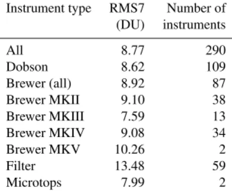
It is also possible to show the performance of the ground networks with this dataset. Table 5 gives the RMS noise of each of the networks versus the MSR level 2 dataset. The Brewer and Dobson datasets show a similar performance, while the Filter instruments show a larger RMS, in accor-dance with the results of Fioletov et al. (2008). The Brewer MKIII (which is still being produced) appears to be the supe-rior instrument. Note again that this RMS also contains con-tributions from the satellite noise and representativity.
How-Table 4. Noise in the satellite dataset with respect to the ground network. RMS1 is before and RMS5 is after the corrections have been applied. RMS6 is the estimate of the noise in the satellite dataset itself.
Name RMS1 RMS5 RMS6
(DU) (DU) (DU)
TOMS2a 8.97 8.76 7.47
TOMS2b 8.98 8.45 7.10
SBUV07 10.01 9.98 8.87
SBUV9a 10.43 10.34 9.27
SBUV9d 9.68 9.64 8.48
SBUV11 9.89 9.82 8.69
SBUV16 9.61 9.33 8.13
GDP 8.89 8.71 7.41
TOGOMI 8.08 7.96 6.51
SGP 9.11 8.92 7.66
TOSOMI 8.66 7.67 6.16
OMDOAO3 8.55 8.17 6.77
OMTO3 6.62 6.48 4.59
GOME2 7.21 6.59 4.74
ever, the relative differences between the ground instruments can be inferred from the table, although there may be geo-graphical differences in the locations of the stations that may somewhat influence the results.
The MSR level 2 data spans 30 years of sequential satellite observations. In this period only 3 time intervals exist with a data gap of more than 2 days. This happened in the period 1995–1996 with gaps of 3.4, 3.0 and 4.5 days.
4 Data assimilation
The satellite instrument observations are combined with me-teorological, chemical and dynamical knowledge of the at-mosphere by using data assimilation. The data assimilation scheme used here is called TM3DAM and is described in Eskes et al. (2003). The chemistry-transport model used in this data assimilation is a simplified version of TM5 (Krol et al., 2005), which is driven by ECMWF analyses of wind, pressure and temperature fields. As input the MSR ozone values and the estimates of the measurement uncertainty are used. These uncertainties are described in Sect. 3.5. A qual-ity screening is implemented to reject unrealistic ozone ob-servations (i.e. below 50 DU or above 700 DU) or unreli-able ozone observations (measured with a solar zenith angle higher than 85◦). Observations that deviate from the model forecasts more than either 3 times the observation uncertainty or 3 times the model uncertainty are also rejected. Because of this restriction and the assumption of unbiased observations, the satellite data has been corrected as described before.
Table 5. Noise figures of the ground network compared to MSR level 2.
Instrument type RMS7 Number of
(DU) instruments
All 8.77 290
Dobson 8.62 109
Brewer (all) 8.92 87
Brewer MKII 9.10 38
Brewer MKIII 7.59 13
Brewer MKIV 9.08 34
Brewer MKV 10.26 2
Filter 13.48 59
Microtops 7.99 2
al. (1986). The model is driven by 6-hourly meteorologi-cal fields (wind, surface pressure, and temperature) of the medium-range meteorological analyses of the ECMWF. The assimilation is using the ERA-40 reanalysis (1978–2001) as well as operational data sets (2002–2008). The 60 or 91 ECMWF hybrid layers between 0.01 hPa and the surface have been converted into the 44 layers used in TM3DAM, whereby in the stratosphere and upper troposphere region all levels of the 60-layer definition are used. The horizontal resolution of the model version used in this study is 2×3◦. This relatively modest resolution is compensated by the prac-tically non-diffusive Prather scheme (with 10 explicit ozone tracers for each grid cell), which allows the model to produce ozone features with a fair amount of detail. The output of the analyses is provided on a grid with a resolution of 1×11/2◦
. Ozone chemistry in the stratosphere is described by two parameterizations. One consists of a linearization of the gas-phase chemistry with respect to production and loss, the ozone amount, temperature and UV radiation. A second parameterization scheme accounts for heterogeneous ozone loss. This scheme introduces a three-dimensional chlorine activation tracer, which is formed when the temperature drops below the critical temperature of polar stratospheric cloud formation. Ozone breakdown occurs in the presence of the chlorine activation tracer, depending on the presence of sunlight. The rate of ozone decrease is described by an exponential decay, with a rate proportional to the amount of activation tracer below the critical temperature and with a minimal decay time of 12 days. The cold tracer is deacti-vated when light is present with a time scale of respectively 5 and 10 days on the Northern and Southern Hemisphere.
The total ozone data are assimilated in TM3DAM by plying a parameterized Kalman filter technique. In this ap-proach the forecast error covariance matrix is written as a product of a time independent correlation matrix and a time-dependent diagonal variance. The various parameters in the approach are fixed and are based on the forecast minus ob-servation statistics accumulated over the period of one year
(2000) using GOME observations. This approach produces detailed and realistic time- and space-dependent forecast er-ror distributions.
The data assimilation approach used for this work is based on the scheme described in (Eskes et al., 2003), but some improvements are made. The most important changes are:
1. The inclusion of a new ozone chemistry parameterisa-tion Cariolle version 2.1 (Cariolle et al., 2007). This up-date of the Cariolle parameterisation has improved the forecast over Antarctica during the ozone hole season. 2. As it was no longer practical to perform the data
assim-ilation on a per-orbit basis, a fixed 30 min data assimi-lation time step has been used.
3. The construction of super-observations from the multi-ple satellite instrument dataset. Previously the error of the super-observation was computed with the assump-tion of a constant observaassump-tion error. In the present multi-sensor analysis an average observation error per instru-ment is introduced (see Table 4). Based on the corre-lations of the GOME observations in a single grid cell, earlier established by Eskes et al. (2003), the average error correlation is assumed to be 50%. The super-observations are average satellite super-observations weighted with the inverse of their variances.
The quality control consisted of a comparison between the individual observations and the model forecast. When this difference exceeded 3 times the forecast error or the observa-tion error, the observaobserva-tion is rejected. Only a few percent of all observations is rejected with this quality check.
One example drawn from the MSR ozone analysis data set is shown in Fig. 3, which shows the MSR ozone field derived for 15 April 1992 and 24 September 2002 at 12:00 UTC. These examples illustrate the resolution of the data set, which allows monitoring events like the split of the ozone hole in 2002. No discontinuity across the date line is present in the images, which is often seen in gridded level 2 data. The 6-hourly instantaneous and monthly mean ozone fields are available on the TEMIS web site, http://www.temis.nl/. For UV radiation studies the daily ozone fields at local noon are also made available on this web site. In Fig. 4 the aver-age ozone mass deficit over Antarctica in the period 21–30 September, when the ozone depletion is usually at its maxi-mum, is shown for the period 1978–2008. The ozone mass deficit is defined as the total amount of ozone needed to fill the ozone columns below 60◦ South to a level of 220 DU.
Fig. 3. Examples of the analysed MSR ozone field in DU. The left panel shows a low pressure system over Western Europe on 15 April 1992. The right panel shows the split ozone hole over Antarctica on 24 September 2002.
0 5 10 15 20 25 30 35 40
1979 1980 1981 198219831984 1985 1986 1987 1988 19891990 1991 1992 1993 1994 19951996 1997 1998 1999 2000 2001 20022003 2004 2005 2006 2007 2008
Year
Ozone mass deficit (million tonnes)
Fig. 4. The ozone mass deficit over Antarctica in the period 21–30 September based on the multi-sensor re-analysis (MSR) total ozone in the period 1979–2008.
dissolved quickly after this event. The maximum daily ozone deficit observed during the 30 year period was 42.2×10⁹kg on 26 September, 2003.
5 Evaluation of the MSR data
Figure 5 gives an example of the MSR level 4 data set com-pared to ground data: it shows the same time period and lo-cation as for Fig. 1. Where Fig. 1 clearly showed systematic deviations, most notable the seasonal cycles, in Fig. 5 no sea-sonal cycle or trends are visible. Still a small offset remains between MSR and the ground observations on this location,
Fig. 5. Monthly averaged anomalies (satellite measurement mi-nus ground measurement) for the overpass data of the MSR at the ground station De Bilt (5.18◦E, 52.1◦N) in the Netherlands.
can no longer be distinguished due to its high concentrations of ground stations. On average no offset is present, and only a few outliers are visible. No systematic structures are obvi-ous in the geographical distribution.
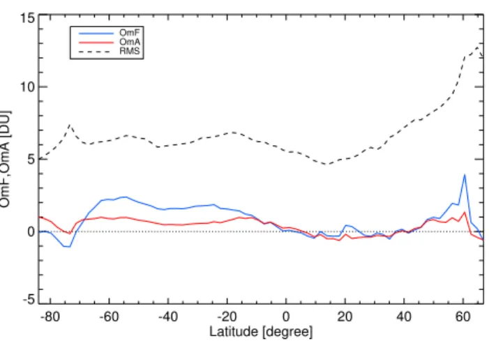
An important source of information for the evaluation of any data assimilation is the observation-minus-forecast (OmF) and the observation-minus-analysis (OmA) statistics produced by the TM3DAM analysis system (“forecast” is the model result just before assimilation and “analysis” is the as-similation result). This mechanism allows detection of sud-den changes in the data quality and provides error estimates for the total ozone retrieval as well as the model performance. The analysis uncertainty is reported as a two-dimensional field, part of the analysis product. In the data assimilation the forecasts are calculated in sequential steps of half an hour. For assimilation of a single sensor, such as TOMS or OMI the observations at a certain location are typically once a day and therefore the OmF and OmA reflect a time step of 1 day. For the assimilation of SBUV only (e.g. beginning 1995), ac-counting for a correlation length of 500 km, the revisit time is typically 1 week. For data assimilation of multiple sensors this is different, time steps between observations can range anything between half an hour and 1 day. This means that the OmF and OmA, and therefore the data assimilation results, are more restrained by the observations. Typical OmF and OmA behaviour that has been checked are: (i) in general the OmA has to be smaller than the OmF, (ii) no geo-location or geo-parameter dependencies have to be visible, (iii) the RMS will mainly reflect the error distribution of the observations.
As example, the OmF and OmA are analyzed for January 2008 as function of location, latitude band, solar zenith an-gle, viewing anan-gle, total ozone and cloud parameters. No significant systematic deviations were found. In Fig. 7 the geographical distribution of the OmF gridded for January 2008 is shown. In general the mean OmF is between−3 and+3 DU. In the northern latitudes some higher variations
Fig. 6. Fitted offset (MSR-ground) between the MSR level 4 data and all selected ground measurement in the period 1978–2008.
-150 -120 -90 -60 -30 0 30 60 90 120 150
-150 -120 -90 -60 -30 0 30 60 90 120 150
-60
-30
0
30
60
-60
-30
0
30
60
-15 -12 -9 -6 -3 0 3 6 9 12 15
Fig. 7. Example of the global distribution, gridded on 1×1◦, of the observation-minus-forecast in DU of the MSR dataset averaged for the month January 2008. The MSR data for this month is based on satellite observations from GOME, SCIAMACHY, GOME2 and OMI.
are found caused by the strong natural variations around the North Pole in this time of the year. No obvious patterns as function of ground elevation or surface type were seen, and the patterns seem to be rather uncorrelated from one month to the next. The OmA for this month was much smaller than the OmF as is to be expected. The distribution of the OmF was found to be close to normal (Gaussian), which means that at least the largest contribution to the OmF error must closely agree with the assumption of Gaussian error distribution.
-80 -60 -40 -20 0 20 40 60 Latitude [degree]
-5 0 5 10 15
OmF,OmA [DU]
OmF OmA RMS
Fig. 8. Observation-minus-forecast in DU (blue line) and observation-minus-analysis (red line) as a function of latitude. The dashed black line represents the RMS value of the observation-minus-forecast distribution. All data are averaged over January 2008.
which is related to high ozone variability in winter, and a cor-responding increase of the representativity mismatch. The bias between the forecast and the columns is smaller than 1%. The bias between analysis and the observations is in general smaller (about 1 DU), which shows the effect of the data assimilation. Compared to assimilation of the observa-tions of the GOME instrument only, as shown earlier in Es-kes et al. (2003) with almost the same data assimilation sys-tem, both RMS and bias are considerably decreased by using an improved retrieval for GOME and by using the full MSR level 2 dataset consisting of GDP, TOGOMI, SGP, TOSOMI, OMDOAO3, OMTO3, GOME2 for January 2008.
In Fig. 9 the OmF is shown as function of solar zenith angle, ozone, cloud fraction and viewing angle for January 2008. Again no large systematic effects are found and similar OmF, OmA and RMS values are found as earlier discussed for Fig. 8. For high solar zenith angles the RMS value in-creases, because these measurements are usually associated with the highly variable ozone concentrations in and around the polar vortex. In addition, the model bias is higher closer to the region of the polar night, where no satellite observa-tions of ozone are performed. From the ozone dependence it follows that the model shows a slight tendency to underesti-mate the range of ozone values.
Similar results as shown in Fig. 9 are found for other months in the data set. The period from June 1993 till May 1995 is of special interest because the satellite observations are sparse as only SBUV9d and SBUV11 performed mea-surements. Note that in this period the forecast of the OmF is for 24 h. Also in this period the mean OmF and OmA val-ues are small (less than 1%), but the RMS valval-ues are higher, up to 4–5%. For this period the forecast error is likely to be higher because of the low coverage of the Earth by the sparse SBUV observations.
20 30 40 50 60 70 80 Solar zenith angle [degree] -5
0 5 10 15
OmF,OmA [DU]
250 300 350 400 450 Ozone [DU] -5
0 5 10 15
OmF,OmA [DU]
20 40 60 80 Cloud fraction [%] -5
0 5 10 15
OmF,OmA [DU]
-60 -40 -20 0 20 40 60 Viewing zenith angle [degree] -5
0 5 10 15
OmF,OmA [DU]
OmF OmA
RMS
a
b
c
d
Fig. 9. The observation-minus-forecast in DU (blue line) and the observation-minus-analysis (red line) as a function of solar zenith angle (a), observed ozone (b), cloud fraction (c), and viewing zenith angle(d). The dashed line represents the RMS value of the observation-minus-forecast distribution. All data are averaged over January 2008.
The assumption has been made that different retrieval datasets from the same satellite instrument have uncorrelated errors. To check this assumption the average correlation of the ozone differences (between satellite observation and analysis) is calculated for different algorithms but from the same satellite observation. Based on the OmA statistics the average correlation of the algorithm pairs TOGOMI/GDP, TOSOMI/SGP and OMDOAO3/OMTO3 were estimated as, respectively, 0.22±0.10, 0.20±0.02 and 0.22±0.03 for April 2007 and 0.34±0.17, 0.30±0.09 and 0.14±0.03 for the month December 2008. From this low correlation we conclude that using the observations of the mentioned algo-rithm pairs as independent data sets in the data assimilation is a valid choice.
6 Conclusions and outlook
By exploiting on the one hand the accuracy and large num-ber of ground measurements and on the other hand the global coverage of satellite observations, a data set is created of an optimal estimate of the global distribution of total ozone in a period of 30 years. The data is created in two steps: firstly, correcting small systematic biases in the satellite data by tak-ing the ground observation on average as the true value. Sec-ondly, all satellite data is assimilated with a Kalman filter technique in order to have a consistent data set with a regular spatial grid of 1×11/2◦and a time step of 6 h throughout the
Several assimilation-based long-term ozone records exist, and have been reported in the literature. Dethof and Holm (2004), report on the quality of a 45-year reanalysis (ERA40) of ozone performed with the ECMWF model. This work is based on previous data versions of TOMS (version 7) and SBUV (version 6), and no additional corrections were ap-plied to account for drifts and offsets against surface data. The 45 years can be divided in four different time windows, depending on the availability of satellite data. The quality of the analyses differs from one window to the next, which complicates the use of this reanalysis for trend studies.
Brunner et al. (2006b) provide a quasi-3D ozone time se-ries for the period 1979–2004, based on the NIWA total ozone dataset constructed from TOMS/SBUV v8 and GOME total ozone observations (Bodeker et al., 2001, 2005). As in the MSR dataset, Dobson ground observations were used to remove offsets and drifts in the satellite data. However, the MSR uses both Dobson and Brewer ground observations for correcting the satellite observations, and these corrections are based on dependencies of parameters directly related to retrieval errors. Important in correcting satellite data is the fitting against the effective ozone temperature, which is a critical parameter for total ozone retrievals. This is a novelty in the MSR data set. The analysis by Brunner et al. (2006b) is based on a two-dimensional equivalent latitude – poten-tial temperature Kalman filter approach. Brunner shows that realistic 3-D ozone distributions can be reconstructed on the basis of 2-D ozone column information only. In the MSR the analyses are performed with a full 3-D model, which avoids errors that may result from the 2-D–3-D mapping. However, the data presented are restricted to the 2-D ozone column field, because this is strongly determined by the satellite ob-servations.
Compared to existing long-term datasets, the MSR data is based on more satellite data sets by including all available retrievals of the recent satellite instruments GOME, SCIA-MACHY, OMI, and GOME-2.
Currently, the MSR data set is used by research institutes for the creation of long-term time series of UV radiance, which will be compared with ground measurements and used for trend analysis. The data is also of interest for climate re-search, for atmospheric chemistry modelling, for analyzing trends in ozone and for the study of the recovery of the ozone hole.
The OmA of this dataset is less than 1%, which is better than for the assimilation of observations of a single sensor. The model influence as estimated by the difference between OmF and OmA is in general very small. Therefore, even for small periods of a couple of days with no data, the bias will remain within 1%. As discussed earlier, this holds also for the period with only sparse SBUV observations. The longest gap in our level 2 data series is 4.5 days. The RMS errors are around 2%, which is low since the RMS errors contain rep-resentativity errors, forecast errors and instrumental noise.
It has been shown that the MSR level 2 data presented no drift and an insignificant SZA and effective ozone tempera-ture dependence as compare to the ground observations (see Table 2). The final MSR level 4 data is on average compa-rable with the ground data: the fitted offset, trend and sea-sonality in the comparison between MSR level 4 data and all observations of the WOUDC data base were negligible. The maximum fitted offset is 0.2 DU. All the systematic effects found in the satellite data are removed by the simple cor-rections (using a few basic parameters) applied to the satel-lite observations in the period 1978–2008. Especially for the last years, the corrections applied to the satellite data are ex-pected to improve when more data will become available in the WOUDC database.
The combination of the different satellite data into a co-herent MSR level 2 data revealed that there are systematic differences between all the total ozone satellite products and the network of ground stations. By combining the satellite data and model knowledge using data assimilation and by us-ing the ground data as a reference the aim was to obtain the best possible data set for the total ozone in the atmosphere by combining all available ozone column information. It is however difficult to draw conclusions about the quality of in-dividual dataset, since our work is based on the assumption that the ground observations are on average without mean bias, seasonal bias or trends. We hope that this work will stimulate the research in retrieval algorithms, both for the satellite and the ground instruments. For future missions we recommend to plan a long repeat cycle of the satellite orbit in such a way that the overpass dataset of a single ground station contains all viewing angles of the satellite.
The authors are aware that at the time of the writing of this paper development is still on-going for the improvement of the retrieval products of in particular GOME-2 and OMI, which are relatively new satellite instruments. But research is also being done to improve the other satellite products, so certain conclusions about their quality will probably be quickly outdated. Therefore, as new developments become available, also the MSR data set is planned to be regularly reprocessed to incorporate the latest versions of satellite and ground data.
Appendix A
Satellite datasets
For each satellite dataset the version number, the origin of the data and a reference is shown. If part of the dataset has been rejected, this is also shown here. The corrections applied to each dataset are shown at the end of each entry. In all for-mulaeXis the total ozone in DU,Teffis the effective ozone
A1 TOMS2a
– Processing: NASA. (Version: 8).
– Downloaded from: http://disc.sci.gsfc.nasa.gov/data/ datapool/TOMS/Level 2/.
– Reference: Bhartia et al., 2002.
– All data with ozone values>0 have been used.
– Corrections applied: effective temperature and offset.
– Xcor=Xsat−0.462·(Teff+46.3)−2.066.
A2 TOMS2b
– Processing: NASA (Version: 8).
– Downloaded from: http://disc.sci.gsfc.nasa.gov/data/ datapool/TOMS/Level 2/.
– Reference: Bhartia et al., 2002.
– All data with ozone values>0 have been used.
– Corrections found: effective ozone temperature, VZA (not linear), trend (from 2000) and offset.
– Before 1 January 2000: Xcorr = Xsat−0.447· (Teff+46.3)+0.839+f (pixel).
– From 1 January 2000: Xcorr =Xsat −0.728 · (Teff+46.3)+5.093·MJ D−8.098+f (pixel).
– The viewing zenith angle correctionf(pixel) as function of the across-track pixel is shown in Fig. A1.
A3 SBUV07, SBUV9a, SBUV9d, SBUV11, SBUV16
– Processing: NOAA/NASA Ozone Processing Team.
– Data from: DVD-ROM “SBUV Version 8” NOAA/NASA.
– Reference: Miller et al., 2002; Taylor et al., 2003.
– All data flagged as “Good retrieval” have been used.
– SBUV data have been corrected for temperature only.
– SBUV07:Xcor=Xsat−0.153·(Teff+46.3)−3.431
– SBUV9a:Xcor=Xsat−0.376·(Teff+46.3)−2.418
– SBUV9d:Xcor=Xsat−0.196·(Teff+46.3)−0.823
– SBUV11:Xcor=Xsat−0.258·(Teff+46.3)−2.360
– SBUV16:Xcor=Xsat−0.467·(Teff+46.3)−6.155
Fig. A1.The viewing angle correction for TOMS2b.
A4 GDP
– Processing: DLR/ESA. (Version: 4.00 and 4.10)
– Data from: http://nlsciadc.knmi.nl/
– Reference: Van Roozendael et al., 2006; Balis et al., 2007a.
– Back-scan pixels have been ignored; ozone values<0 have been ignored.
– Both a SZA, VZA correction has been applied, the last nonlinear (pixel based, thee values).
– Deleted: June–September 2003.
– Xcor=Xsat−0.114·(SZA−30)+2.933+f (pixel).
– The viewing zenith angle correctionf(pixel) as function of the across-track pixel is given by Table A1.
A5 TOGOMI
– Processing: KNMI. (Version 1.2, level 1: version 3.02).
– Data from: http://www.temis.nl/protocols/O3total.html.
– Reference: Valks et al., 2004.
– All data have been used (there are no back-scan pixels in the dataset).
– A nonlinear VZA dependence has been corrected (pixel based, six values).
– Xcor=Xsat+1.649+f (pixel).
Table A1. The viewing angle as function of pixel for the GDP data set.
Pixel East Centre West
Correction (DU) −1.17 0.42 0.89
Table A2. The correction (DU) as function of view angle for the TOGOMI data set.
Mode Pixel
East Centre West
Normal −1.76 0.40 1.47
Small-swath 0.04 0.99 0.56
Nadir static 0 0 0
Polar viewing 0 0 0
A6 SGP
– Processing: DLR/ESA (Version 3.01).
– Data from: http://nlsciadc.knmi.nl/.
– Reference: Lerot et al., 2009; Lambert et al., 2007.
– Back-scan pixels have been ignored; ozone values<0 have been ignored.
– This product shows a significant trend. A small VZA dependence has also been corrected.
– Xcor=Xsat−0.016·VZA−8.031+1.090·MJD
A7 TOSOMI
– Processing: KNMI (version 0.43, level 1: version 6.03)
– Data from: http://www.temis.nl/protocols/O3total.html.
– Reference: Eskes et al., 2005.
– All data have been used (there are no back-scan pixels in the dataset).
– This product has a trend similar to SGP. Also small SZA and VZA corrections have been applied.
– Deleted: 20 December 2002–29 December 2002.
– Xcor=Xsat−0.284·(SZA−30)+0.049·VZA+1.039·
MJD+2.322
Fig. A2.The viewing angle correction for GOME2.
A8 OMDOAO3
– Processing: NASA (Version: 003, level 1: collection 3).
– Data from: http://www.temis.nl/protocols/O3total.html.
– Reference: Veefkind et al., 2006; Balis et al., 2007b; McPeters et al., 2008.
– Pixels have been deleted if ozone values are zero, or the RMS errors are higher than 10 DU, or the logical sum of “ProcessingQualityFlags” and “10 911” is nonzero.
– The instrument is developing “row anomalies”. Bad rows have been deleted according to the infor-mation on http://www.knmi.nl/omi/research/product/ rowanomaly-background.php. A procedure for the “zoom mode” has been indirectly derived from this in-formation.
– Corrections: SZA (not linear), temperature, trend, off-set.
– Xcor = Xsat − 0.00189 · (SZA−30)2 + 0.300 · (Teff+46.3)−0.358·MJD+5.379
A9 OMTO3
– Processing: NASA. (Version 3, level 1: collection 3).
– Data from: http://disc.sci.gsfc.nasa.gov/Aura/ data-holdings/OMI/omto3 v003.shtml.
– Reference: Bhartia et al., 2002; Balis et al., 2007b; McPeters et al., 2008.
– Pixels have been deleted if total ozone is less then 1 DU, or the logical sum of “Quality Flags” and hexadecimal “FFF6” is nonzero.
– All data before 9 September 2004 have been ignored.
– Corrections: temperature, offset.
– Xcor=Xsat−0.282·(Teff+46.3)+2.578
A10 GOME2
– Processing: DLR/EUMETSAT. (Versions: GDP 4.3, using reprocessed level1B-R1 v4.0 data).
– Data from: DLR (provided by P. Valks).
– Reference: Valks et al., 2008; http://lap.physics.auth.gr/ eumetsat/.
– GOME-2 appears to have a significant trend. Also cor-rections for SZA and VZA (nonlinear) have been ap-plied.
– Xcor=Xsat−0.164·SZA−2.186·MJD+26.998+
f (pixel).
– The viewing zenith angle correctionf(pixel) as function of the across-track pixel is shown in Fig. A2.
Acknowledgements. The authors would like to thank Pieter Valks for providing us the GOME-2 ozone column data. The authors thank the WOUDC and the ground station operators for providing the ozone column data at http://www.woudc.org/. Furthermore, the authors thank the agencies NASA, NOAA, ESA, and EUMETSAT for making respectively the TOMS and OMI data, the SBUV data, the GOME and SCIAMACHY data, and the GOME-2 data publicly available at their web sites. We thank Piet Stammes for his help with the manuscript.
Edited by: M. Van Roozendael
References
Balis, D., Lambert, J.-C., Van Roozendael, M., Spurr, R., Loyola, D., Livschitz, Y., Valks, P., Amiridis, V., Gerard, P., Granville, J., and Zehner, C.: Ten years of GOME/ERS-2 total ozone data – The new GOME data processor (GDP) version 4: 2. Ground-based validation and comparisons with TOMS V7/V8, J. Geo-phys. Res., 111, D07307, doi:10.1029/2005JD006376, 2007a. Balis, D., Kroon, M., Koukouli, M. E., Brinksma, E. J.,
Labow, G., Veefkind, J. P., and McPeters, R. D.:
Vali-dation of Ozone Monitoring Instrument total ozone column measurements using Brewer and Dobson spectrophotometer ground-based observations, J. Geophys. Res., 112, D24S46, doi:10.1029/2007JD008796, 2007b.
Bhartia, P. K. and Wellemeyer, C.: TOMS-V8 total O3 algorithm, in OMI Algorithm Theoretical Basis Document, vol. II, OMI Ozone Products, ATBD-OMI-02, edited by P. K. Bhartia, 15–31, NASA Goddard Space Flight Cent., Greenbelt, Md., http://eospso.gsfc. nasa.gov/eos homepage/for scientists/atbd/, 2002.
Bodeker, G. E., Scott, J. C., Kreher, K., and McKenzie, R. L.: Global ozone trends in potential vorticity coordinates using TOMS and GOME intercompared against the Dobson network: 1978–1998, J. Geophys. Res., 106(D19), 23029–23042, 2001.
Bodeker, G. E., Shiona, H., and Eskes, H.: Indicators of
Antarctic ozone depletion, Atmos. Chem. Phys., 5, 2603–2615, doi:10.5194/acp-5-2603-2005, 2005.
Bovensmann, H., Burrows, J. P., Buchwitz, M., Frerick, J., No¨el, S., Rozanov, V. V., Chance, K. V., and Goede, A. P. H.: SCIA-MACHY: Mission Objectives and Measurement Modes, J. At-mos. Sci., 56, 127–150, 1999.
Brunner, D., Staehelin, J., Maeder, J. A., Wohltmann, I., and Bodeker, G. E.: Variability and trends in total and vertically re-solved stratospheric ozone based on the CATO ozone data set, Atmos. Chem. Phys., 6, 4985–5008, doi:10.5194/acp-6-4985-2006, 2006a.
Brunner, D., Staehelin, J., K¨unsch, H.-R., and Bodeker, G. E.: A Kalman filter reconstruction of the vertical ozone distribu-tion in an equivalent latitude-potential temperature framework from TOMS/GOME/SBUV total ozone observations, J. Geo-phys. Res., 111, D12308, doi:10.1029/2005JD006279, 2006b. Burrows, J. P., Weber, M., Buchwitz, M., Rozanov, V.,
Ladst¨atter-Weißenmayer, A., Richter, A., De Beek, R., Hoogen, R., Bram-stedt, K., Eichmann, K. U., Eisinger, M., and Perner, D.: The Global Ozone Monitoring Experiment (GOME): Mission Con-cept and First Scientific Results, J. Atmos. Sci., 56, 151–175, 1999.
Callies, J., Corpaccioli, E., Eisinger, M., Hahne, A., and Lefebvre, A.: GOME-2 – Metop’s Second Generation sensor for Opera-tional Ozone Monitoring, ESA Bulletin, 102, 2000
Cariolle, D. and Teyss`edre, H.: A revised linear ozone photochem-istry parameterization for use in transport and general circula-tion models: multi-annual simulacircula-tions, Atmos. Chem. Phys., 7, 2183–2196, doi:10.5194/acp-7-2183-2007, 2007.
Derber, J. C. and Wu, W.-S.: The Use of TOVS Cloud-Cleared Ra-diances in the NCEP SSI Analysis System, Mon. Weather Rev., 126, 2287–2299, 1998.
Dethof, A. and H´olm, E. V.: Ozone assimilation in the ERA-40 re-analysis project, Q. J. Roy. Meteor. Soc., 130, 2851–2872, 2004. Eskes, H. J., van Velthoven, P. F. J., Valks, P. J. M. and Kelder, H. M.: Assimilation of GOME total ozone satellite observations in a three-dimensional tracer transport model, Q. J. Roy. Meteorol. Soc., 129, 1663–1681, 2003.
Eskes, H. J., van der A, R. J., Brinksma, E. J., Veefkind, J. P., de Haan, J. F., and Valks, P. J. M.: Retrieval and valida-tion of ozone columns derived from measurements of SCIA-MACHY on Envisat, Atmos. Chem. Phys. Discuss., 5, 4429– 4475, doi:10.5194/acpd-5-4429-2005, 2005.
Fioletov, V. E., Bodeker, G. E., Miller, A. J., McPeters, R.
D., and Stolarski, R. S.: Global and zonal total ozone
variations estimated from ground-based and satellite
mea-surements: 1964–2000, J. Geophys. Res 107(D22), 4647,
doi:10.1029/2001JD001350, 2002.
Fioletov, V. E., Labow, G., Evans, R., Hare, E. W., K¨ohler, U., McElroy, C. T., Miyagawa, K., Redondas, A., Savastiouk, V., Shalamyansky, A. M., Staehelin, J., Vanicek, K., and Weber, M.: Performance of the ground-based total ozone network as-sessed using satellite data, J. Geophys. Res., 113, D14313, doi:10.1029/2008JD009809, 2008.
Fortuin, J. P. F. and Kelder, H.: “An ozone climatology base on ozonesonde and satellite measurements”, J. Geophys. Res., 103,
31709–31734, available at: http://www.temis.nl/data/fortuin.
Geer, A. J., Lahoz, W. A., Bekki, S., Bormann, N., Errera, Q., Es-kes, H. J., Fonteyn, D., Jackson, D. R., JucEs-kes, M. N., Massart, S., Peuch, V.-H., Rharmili, S., and Segers, A.: The ASSET in-tercomparison of ozone analyses: method and first results, At-mos. Chem. Phys., 6, 5445–5474, doi:10.5194/acp-6-5445-2006, 2006.
Harris, N. R. P., Kyr¨o, E., Staehelin, J., Brunner, D., Andersen, S.-B., Godin-Beekmann, S., Dhomse, S., Hadjinicolaou, P., Hansen, G., Isaksen, I., Jrrar, A., Karpetchko, A., Kivi, R., Knudsen, B., Krizan, P., Lastovicka, J., Maeder, J., Orsolini, Y., Pyle, J. A., Rex, M., Vanicek, K., Weber, M., Wohltmann, I., Zanis, P., and Zerefos, C.: Ozone trends at northern mid- and high lati-tudes – a European perspective, Ann. Geophys., 26, 1207–1220, doi:10.5194/angeo-26-1207-2008, 2008.
Kerr, J. B.: New methodology for deriving total ozone and
other atmospheric variables from Brewer spectrophotome-ter direct sun spectra, J. Geophys. Res., 107(D23), 4731, doi:10.1029/2001JD001227, 2002.
Kiesewetter, G., B.-M. Sinnhuber, M. Vountas, M. Weber, and J. P. Burrows, A long-term stratospheric ozone data set from assimi-lation of satellite observations: High-latitude ozone anomalies, J. Geophys. Res., 115, D10307, doi:10.1029/2009JD013362, 2010. Krol, M., Houweling, S., Bregman, B., van den Broek, M., Segers, A., van Velthoven, P., Peters, W., Dentener, F., and Bergamaschi, P.: The two-way nested global chemistry-transport zoom model TM5: algorithm and applications, Atmos. Chem. Phys., 5, 417– 432, doi:10.5194/acp-5-417-2005, 2005.
Krzy´scin, J. W.: Statistical reconstruction of daily total ozone over Europe 1950 to 2004, J. Geophys. Res., 113, D07112, doi:10.1029/2007JD008881, 2008.
Lambert, J.-C., Granville, J., Lerot, C., Gerard, P., Fayt, C., Van Roozendael, M. and the ACVT/GBMCD Ozone Column Team: GDP 4.0 transfer to SGP 3.0 for SCIAMACHY ozone column processing: verification with SDOAS/GDOAS prototype algo-rithms and delta-validation with NDACC and WOUDC network data, Proceedings of the Third Workshop on the Atmospheric Chemistry Validation of ENVISAT (ACVE-3), 4-7 Dec. 2006, ESA/ESRIN, Frascati, Italy, ESA Publications Division Special Publication SP-642 (CD), 2007.
Lerot, C., Van Roozendael, M., van Geffen, J., van Gent, J., Fayt, C., Spurr, R., Lichtenberg, G., and von Bargen, A.: Six years of total ozone column measurements from SCIAMACHY nadir observations, Atmos. Meas. Tech., 2, 87–98, doi:10.5194/amt-2-87-2009, 2009.
Levelt, P. F., van den Oord, G. H. J., Dobber, M. R., M¨alkki, A., Visser, H., de Vries, J., Stammes, P., Lundell, J., and Saari, H.: The Ozone Monitoring Instrument, IEEE T. Geoscu. Remote, 44(5), 1093–1101, doi:10.1109/TGRS.2006.872333, 2006. Lindfors, A., Tanskanen, A., Arola, A., van der A, R., Bais, A.,
Feister, U., Janouch, M., Josefsson, W., Koskela, T., Lakkala, K., den Outer, P. N., Smedley, A. R. D., Slaper, H., and Webb, A. R.: The PROMOTE UV Record: Toward a Global Satellite-Based Climatology of Surface Ultraviolet Irradiance, IEEE Journal of Selected Topics in Applied Earth Observations and Remote Sens-ing, 2(3), 207–212, doi:10.1109/JSTARS.2009.2030876, 2009. M¨ader, J. A., Staehelin, J., Brunner, D., Stahel, W. A., Wohltmann,
I., and Peter, T.: Statistical modeling of total ozone: Selec-tion of appropriate explanatory variables, J. Geophys. Res., 112, D11108, doi:10.1029/2006JD007694, 2007.
McPeters, R. D. and Labow, G. J.: An assessment of the accuracy of 14.5 years of Nimbus 7 TOMS version 7 ozone data by com-parison with the Dobson network, Geophys. Res. Lett., 23(25), 3695–3698, 1996.
McPeters, R., Kroon, M., Labow, G., Brinksma, E., Balis, D., Petropavlovskikh, I., Veefkind, J. P., Bhartia, P. K., and Lev-elt, P. F.: Validation of the Aura Ozone Monitoring Instrument total column ozone product, J. Geophys. Res., 113, D15S14, doi:10.1029/2007JD008802, 2008.
Miller, A. J., Nagatani, R. M., Flynn, L. E., Kondragunta, S., Beach, E., Stolarski, R., McPeters, R. D., Bhartia, P. K., De-Land, M. T., Jackman, C. H., Wuebbles, D. J., Patten, K. O., and Cebula, R. P.: A cohesive total ozone data set from the SBUV(/2) satellite system, J. Geophys. Res., 107(D23), 4701, doi:10.1029/2001JD000853, 2002.
Prather, M. J.: Numerical advection by conservation of ozone data in weather-prediction models, Q. J. Roy. Meteorol. Soc., 122, 1545–1571, 1986.
Randel, W. J., Shine, K. P., Austin, J., Barnett, J., Claud, C., Gillett, N. P., Keckhut, P., Langematz, U., Lin, R., Long, C., Mears, C., Miller, A., Nash, J., Seidel, D. J., Thompson, D. W. J., Wu, F., and Yoden, S.: An update of observed strato-spheric temperature trends, J. Geophys. Res., 114, D02107, doi:10.1029/2008JD010421, 2009.
Redondas, A. and Cede, A.: Brewer algorithm sensitivity analy-sis, SAUNA workshop, Puerto de la Cruz, Tenerife, November, 2006.
Reinsel, C. G., Miller, A. J., Weatherhead, E. C., Flynn, L. E., Na-gatani, R. M., Tiao, G. C., and Wuebbles, D. J.: Trend analysis of total ozone data for turn- around and dynamical contributions, J. Geophys. Res., 110, D16306, doi:10.1029/2004JD004662, 2005. Stajner, I., Wargan, K., Pawson, S., Hayashi, H., Chang, L.-P., Hud-man, R. C., Froidevaux, L., Livesey, N., Levelt, P. F., Thompson, A. M., Tarasick, D. W., St¨ubi, R., Andersen, S. B., Yela, M., K¨onig-Langlo, G., Schmidlin, F. J., and Witte, J. C.: Assimi-lated ozone from EOS-Aura: Evaluation of the tropopause re-gion and tropospheric columns, J. Geophys. Res., 113, D16S32, doi:10.1029/2007JD008863, 2008.
Staehelin, J., Harris N. R. P., Appenzeller, C., and Eberhard, J.: Ozone Trends: A Review, Rev. Geophys., 39(2), 231–290, 2001. Staehelin, J., Kerr, J., Evans, R., and Vanicek, K.: Comparison of to-tal ozone measurements of Dobson and Brewer spectrophotome-ters and recommended transfer functions, Tech. Rep., WMO, World Meteorological Organization Global Atmosphere Watch (WMO-GAW) Report 149, 2003.
Stolarski, R. S., Bloomfield, P., McPeters, R. D., and Herman, J. R.: Total Ozone trends deduced from Nimbus 7 Toms data, Geophys. Res. Lett., 18(6), 1015–1018, 1991.
Stolarski, R. S., Labow, G. J., and McPeters, R. D.: Springtime Antarctic total ozone measurements in the early 1970s from the BUV instrument on Nimbus 4, Geophys. Res. Lett., 24(5), 591– 594, 1997.
Stolarski, R. S. and Frith, S. M.: Search for evidence of trend slow-down in the long-term TOMS/SBUV total ozone data record: the importance of instrument drift uncertainty, Atmos. Chem. Phys., 6, 4057–4065, doi:10.5194/acp-6-4057-2006, 2006a.
Taylor, S. L., Cebula, R. P., Deland, M. T., Huang, L.-K., Sto-larski, R. S., and McPeters, R. D.: Improved calibration of NOAA-9 and NOAA-11 SBUV/2 total ozone data using in-flight validation methods, Int. J. Remote Sens., 24.2, 315–328, doi:10.1080/01431160304977, 2003.
Valks, P. J. M., De Haan, J. F., Veefkind, J. P., Van Oss, R. F., and Balis, D. S.: TOGOMI: An improved total ozone re-trieval algorithm for GOME, XX Quadrennial Ozone Sympo-sium, 1/6/2004-8/6/2004, edited by: Zerefos, C. S., Athens, Uni-versity of Athens, 129–130, 2004.
Valks, P. J. M., Loyola, D., Hao, N., and Rix, M.: Algorithm The-oretical Baseline Document for GOME-2 total column products of ozone, minor trace gases, and cloud properties, DLR/GOME-2/ATBD/01, 2008.
Van Roozendael, M., Loyola, D., Spurr, R., Balis, D., Lam-bert, J.-C., Livschitz, Y., Valks, P., Ruppert, T., Kenter, P., Fayt, C., and Zehner, C.: Ten years of GOME/ERS-2 total ozone data – The new GOME data processor (GDP) version 4: 1. Algorithm description, J. Geophys. Res., 111, D14311, doi:10.1029/2005JD006375, 2006.
Veefkind, J. P., de Haan, J. F., Brinksma, E. J., Kroon, M., and Lev-elt, P. F.: Total Ozone from the Ozone Monitoring Instrument (OMI) Using the DOAS technique, IEEE T. Geosci. Remote, 44(5), 1239–1244, doi:10.1109/TGRS.2006.871204, 2006. WMO (World Meteorological Organisation), Scientific Assessment
of Ozone Depletion: 2006, Global Ozone Research and Moni-toring Project – Report No. 50, 572 pp., Geneva, Switzerland, 2007.