DEVELOPMENT OF LARGE AREA COVERING HEIGHT MODEL
K. Jacobsen
Leibniz University Hannover, Institute of Photogrammetry and Geoinformation, Germany;
jacobsen@ipi.uni-hannover.de
ISPRS WG IV/2
KEY WORDS: DEM/DTM, image, SAR, Bathymetry, Analysis
ABSTRACT:
Height information is a basic part of topographic mapping. Only in special areas frequent update of height models is required, usually the update cycle is quite lower as for horizontal map information. Some height models are available free of charge in the internet; for commercial height models a fee has to be paid. Mostly digital surface models (DSM) with the height of the visible surface are given and not the bare ground height, as required for standard mapping. Nevertheless by filtering of DSM, digital terrain models (DTM) with the height of the bare ground can be generated with the exception of dense forest areas where no height of the bare ground is available. These height models may be better as the DTM of some survey administrations. In addition several DTM from national survey administrations are classified, so as alternative the commercial or free of charge available information from internet can be used.
The widely used SRTM DSM is available also as ACE-2 GDEM corrected by altimeter data for systematic height errors caused by vegetation and orientation errors. But the ACE-2 GDEM did not respect neighbourhood information. With the worldwide covering TanDEM-X height model, distributed starting 2014 by Airbus Defence and Space (former ASTRIUM) as WorldDEM, higher level of details and accuracy is reached as with other large area covering height models. At first the raw-version of WorldDEM will be available, followed by an edited version and finally as WorldDEM-DTM a height model of the bare ground. With 12m spacing and a relative standard deviation of 1.2m within an area of 1° x 1° an accuracy and resolution level is reached, satisfying also for larger map scales. For limited areas with the HDEM also a height model with 6m spacing and a relative vertical accuracy of 0.5m can be generated on demand.
By bathymetric LiDAR and stereo images also the height of the sea floor can be determined if the water has satisfying transparency. Another method of getting bathymetric height information is an analysis of the wave structure in optical and SAR-images.
An overview about the absolute and relative accuracy, the consistency, error distribution and other characteristics as influence of terrain inclination and aspects is given. Partially by post processing the height models can or have to be improved.
1. INTRODUCTION
The time consuming and partially expensive generation of large area covering digital height models (DHM) can be avoided by use of free of charge or commercially available DHM if they meet the requirements. Not only the absolute and relative accuracy is important, also the point spacing, definition as Digital Terrain Models (DTM) with points on the bare ground or as Digital Surface Models (DSM) with heights of the visible surface – on top of vegetation and building –, homogeneity, support by error map, actuality and percentage of blunders, advantages and disadvantages, limitations in special areas as cities, steep mountains or deserts as well as required post-processing are important. The data acquisition with the possibility to penetrate cloud coverage is an advantage of Synthetic Aperture Radar (SAR), leading to higher homogeneity as optical images. On the other hand based on very high resolution satellite imagery height accuracy and details may exceed the specification for height models from survey administrations. Height models from survey administrations are usually DTM with the advantage of reduced update requirement because vegetation and buildings are changing usually faster as the terrain itself with the exception of areas with strong erosion or subsidence in mining areas. The
reference of the DHM as ellipsoidal or geoid height has to be respected, but a transformation based on geoid is simple.
2. SPECIFICATION OF HEIGHT MODELS The term accuracy for a height model is complex - the terms shown in table 1 are used, so it has to be specified which term is used, just to talk about accuracy cannot be accepted. In addition SZ and NMAD should have the same size if the discrepancies are normal distributed, but for real data this is usually not the case (Höhle et al. 2009).
figures definition RMSZ Square mean of discrepancies
SZ Square mean of (discrepancies – bias) MAD Medium absolute deviation (linear)
NMAD MAD related to 68% probability (MAD*1.48) LE50 Median value of discrepancies
LE90 Threshold including 90% of discrepancies LE95 Threshold including 95% of discrepancies Table 1: accuracy figures
If a height model is compared with a reference height model, usually more large discrepancies as corresponding to the normal
distribution caused by influence of terrain slope and a not avoidable percentage of blunders (Jacobsen 2013). The frequency distribution of the discrepancies fit quite better to the normal distribution based on Normalized Medium Absolute Deviation (NMAD) as based on Standard deviation of height discrepancies (SZ), justifying the use of NMAD as accuracy criteria. The Linear Error for 90% probability (LE90) or for 95%, being 1.65 times respectively 1.96 times larger as SZ in case of normal distributed discrepancies are just defined by 10% respectively 5% of the discrepancies and are strongly depending upon the percentage of blunders and do not describe the frequency distribution of the discrepancies. These values should be avoided.
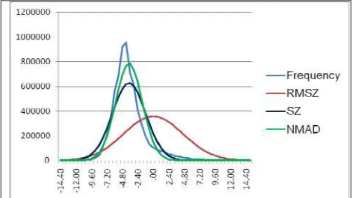
Figure 1: frequency distribution of discrepancies of SRTM DSM against reference DEM in open areas and normal distribution based on RMSZ, SZ and NMAD, test area Warsaw
Figure 1 demonstrates the situation of different accuracy figures at the example of the SRTM height model in test area Warsaw, limited to the open area – without forest, but with small tree groups and limited number of buildings. The frequency distribution has a bias of -3.76m which influences the root mean square error. The standard deviation is related to the bias as well as NMAD. As the overlaid normal distribution based on SZ and NMAD show, more large height discrepancies are included as corresponding to normal distribution, influencing the value of SZ stronger as the linear NMAD. The normal distribution based on NMAD describes the real frequency distribution better as the other figures – this is a typical situation.. In this case RMSZ has a value of 4.57m, SZ 2.60m and NMAD 2.08m. LE90 with 6.44m and LE95 with 7.08m have not so much to do with the characteristics of the height discrepancies and should not be used.
3. ANALYZED DATA SETS 3.1 Overview
The world-wide old GTOPO30 of the USGS and US NGA has been replaced by the GMTED2010 which is available also with 7.5 arc-seconds (arcsec) point spacing, corresponding to 231m at the equator (Danielson & Gesch 2011). For large areas GMTED2010 is using the SRTM-height model. By interferometric synthetic aperture radar (InSAR) based on the Shuttle Radar Topography Mission (SRTM) in 2000 a height model was generated for the area from 56° Southern up to 60° Northern latitude (http://dds.cr.usgs.gov/srtm/version2_1/ SRTM3). For several years the SRTM height model was the most accurate large area covering height model and has been used intensively. 94.5% of the covered land area has been mapped at least twice from different directions, reducing the shadow areas. Even for 50% of the area three or more coverage are available. The SRTM height model has been improved by
gap-filling, editing of spikes and wells in addition to water body levelling since 2009 as Version 2.1. The used C- and X-band cannot penetrate the vegetation, in forest areas it describes the canopy height with 20% up to 30% of the tree height lower, but it is far away from a DTM. Of course by filtering from a DSM a DTM can be generated, but only in open areas, not in closed forest areas without any point located on the bare ground. Supported by the European Space Agency (ESA), ESRIN the SRTM height model has been corrected by satellite radar altimeter data from ERS-1, ERS-2, EnviSat and TOPEX (Smnith and Berry 2011). The altimeter data are able to penetrate vegetation, enabling the change of the SRTM-data from a DSM to a DTM as Altimeter Corrected Elevation 2 (ACE2) Global Digital Elevation Model (GDEM). The ACE2 GDEM with a spacing of 3 arcsec is available free of charge in the WEB (http://tethys.eaprs.cse.dmu.ac.uk/ACE2/login). With higher resolution of 1 arcsec the ASTER GDEM-2 DSM based on the Japanese optical stereo sensor ASTER, on the US platform Terra, has been generated. All available stereo models have been used (Tetsushi 2011). ASTER GDEM is covering the range of the latitude from +83° up to -83°. In the first version the three-dimensional shifts of the individual height models have not been respected correctly, leading to a loss of resolution of the height models (not so detailed contour lines as corresponding to the spacing). By this reason an improved version, the ASTER GDEM2 has been generated and is available free of charge since 2011. ASTER GDEM2 is a product of the Japanese METI and the US NASA (http://www.gdem.aster.ersdac.or.jp/login.jsp).
In addition to the above mentioned free of charge available data also other height models can be bought. SPOT 5 carries in addition to the large HRG instruments the HRS (High Resolution Stereo), a stereo sensor with 5m x 10m GSD and a base to height relation of 1:1.2, used for the generation of height models as SPOT DEM or Reference 3D for large parts of the world with 30m spacing (http://www.astrium-geo.com/en/198-elevation30) (Jacobsen 2004).
The company GAF in cooperation with the German Aerospace Center (DLR) offers the height model EuroMaps 3D with 5m ground spacing based on the Indian optical stereo satellite Cartosat-1 (named also IRS P5). With this stereo satellite, having 2.5m ground resolution, nearly the whole world has been covered (Jacobsen 2006).
The German SAR-satellites TerraSAR-X and TanDEM-X are flying in a close configuration since 2010 for the generation of a nearly worldwide DEM coverage, which will be available starting 2014. This height model will be distributed as WorldDEM by Airbus Defence and Space (former ASTRIUM) with 12m point spacing and a claimed relative standard deviation within a 1° x 1° grid (111²km² at the equator) of 1.2m. On request also data with 6m point spacing will be available.
3.2 GMTED2010
GMTED2010, covering the whole world, is available with 30, 15 and 7.5 arc-seconds point spacing. It is available with different versions – DCS, MAX, MIN, MED, MEA and STD. STD is the quality layer including the estimated local standard deviation, while all other are height models. The DSC-file contains the best information about the DSM, the justification of the other height model versions is hardly to be understand. The DCS-DSM corresponds to the SRTM-height model, but has a lower resolution. Only in areas not covered by SRTM the use of this height model is justified.
3.3 SRTM
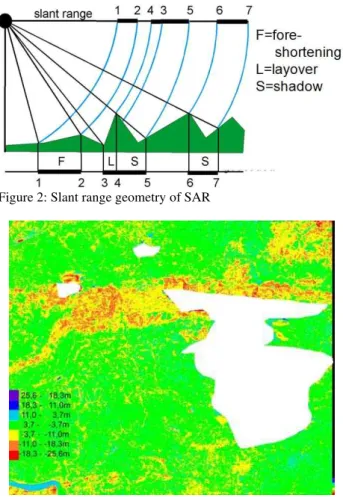
The Shuttle Radar Topography Mission (SRTM) in February 2000 used InSAR. In radar interferometry - two synthetic aperture radar images are taken from slightly different locations. In the Space Shuttle an antenna was mounted in the cargo bay and another the end of a 60m mast. In both locations an X-band antenna and a band antenna were located. The C-band data, operated in the scan-SAR-mode, have been handled by the USA, while the X-band data handled by Italy and Germany only used the strip-map mode. The C-band covered 80% of the Earth surface with 30 m resolution from 56° Southern up to 60.25° Northern latitude, while the X-band during the short mission time covered only parts of this. With the exception of the USA the SRTM C-band height model is available free of charge but to 3 arcsec (~91m at the equator), while the X-band data are available with 1 arcsec spacing. As all InSAR-height models SRTM is influenced by the SAR imaging geometry. SAR images are based on distances, the so called slant range. For a separation of the objects an inclined view is necessary, causing viewing shadows especially for larger nadir angle and layover especially for closer nadir view (see figure 2). Layover is a problem in mountainous areas, but also in cities, overlaying the return signal from different object parts, which cannot be separated later, causing data gaps. These gaps have been filled with other data, especially SPOT-5 HRS height data.
Figure 2: Slant range geometry of SAR
Figure 3: color coded height differences SRTM DSM against reference DTM, Pennsylvania – white = no data
Typical height discrepancies of SRTM DSM against a reference DTM are shown in figure 3. In open area the height discrepancies are limited with values between +/-3.7m (green
color); in forest areas systematic height discrepancies exceeding 3.7m (yellow, orange and red) exist.
Based on satellite radar altimeter data ACE2 GDEM tried to correct SRTM DSM to a SRTM DTM and to solve problems of SRTM orientation errors. Especially in the tropical rainforest this shall lead to the up to now difficult terrain height information. ACE2 GDEM includes also a quality matrix to specify the results.
Figure 4: height difference ACE2 GDEM against reference DTM, Pennsylvania
Figure 4 shows the discrepancies of ACE2 GDEM against the reference DTM in a forest region of Pennsylvania, corresponding to figure 3. The corrections of strips from North-West to South-East are obvious. The original SRTM height model shows larger discrepancies (figure 3), but the correction of ACE2 DTM has been done only partially as obvious in figure 4. Of course by special filtering the shown problem can be solved, but this is different from area to area and usually no reference file is available to check the problems.
RMSZ bias SZ NMAD
ACE all 3.12 1.74 2.58 2.05
SRTM all 6.44 -1.75 6.20 4.11
ASTER all 4.65 -0.25 4.65 3.86
ACE open 7.10 -0.14 7.10 3.19
SRTM open 3.42 -0.63 3.36 2.53
ASTER open 6.37 -1.20 6.25 3.69
Table 1: accuracy in relation to reference data – for the whole area and only for the open area, test field Pennsylvania [m]
On the first view the table 1 seems not to be logic, but it is confirmed by other test areas. ACE2 GDEM has been especially improved in forest areas, but in open areas sometimes a reduction of the accuracy appeared – caused by some not justified corrections. For SRTM the relation is as expected, for ASTER the relation only with NMAD corresponds to the expectation. As mentioned before NMAD expresses the frequency distribution of the height discrepancies quite better as the other values.
RMSZ bias SZ NMAD
ACE all 4.60 1.14 4.45 3.96
SRTM all 5.06 2.05 4.63 4.11
ASTER all 10.18 0.18 10.18 9.16
ACE open 3.91 2.50 3.00 2.70
SRTM open 4.56 3.75 2.59 2.10
ASTER open 9.68 1.96 9.48 8.06
Table 1: accuracy in relation to reference data – for the whole area and only for the open area, test field Warsaw [m]
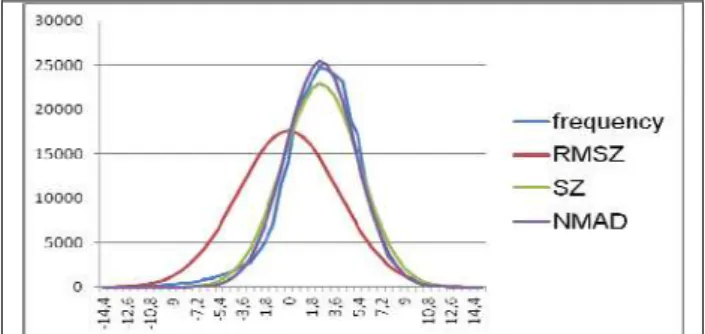
In the flat test area Warsaw, with just 22% of the area covered by forest, with ACE2 GDEM better results as with SRTM has been achieved for the whole area including forest. In the open area RMSZ for ACE2 GDEM is better as for SRTM because of the improved bias. The relative accuracy without the bias (SZ and NMAD) for SRTM are better as for ACE2 GDEM as in the Pennsylvania test area. The results for ASTER are not as good because of the limited number of stacks available in this area. The frequency distribution of the height discrepancies together with the overlaid normal distributions (figure 5) again are typical – the normal distribution based on NMAD fits better to the frequency distribution as the normal distribution based on SZ, RMSZ is shifted by the bias.
Figure 5: frequency distribution of discrepancies of ACE2 GDEM against reference DEM in open areas and normal distribution based on RMSZ, SZ and NMAD, test area Warsaw
These both test areas show the general trend for the mentioned 3 height models, confirmed by other test areas. ACE2 GDEM has advantages in overall areas including forest; nevertheless the relative accuracy is not optimal because of only partial correction (figure 4). In open areas ACE2 GDEM sometimes has the advantage of lower bias, caused by height correction, but without the bias SZ and NMAD are better for SRTM. ASTER GDEM2 is strongly influenced by the number of used stacks (number of used images), but in areas of satisfying number of stacks the point spacing of 1 arcsec leads to better morphologic details as SRTM and ACE2 GDEM with 3 arcsec. Up to now only average height accuracy for the test blocks is shown, but in any case a dependency of the geometric quality upon the terrain inclination in the form: SZ = A + B∗tan(slope) exists. The factor B depends upon the resolution of the height model, possible remaining shifts of the DEM, the terrain and the inclination itself – for flat areas the factor cannot be determined. For SRTM the factor B is in the range of 10m to 50m, for ASTER GDEM2 in the range of 10m to 30m, for SPOT 5 HRS in the range of 5m to 20m and for Cartosat-1 in the range of 5m to 15m. For flat areas the accuracy is better as the overall accuracy. For ASTER GDEM2 the accuracy strongly depends upon the number of stacks (number of used images for the height information). In (Jacobsen, Passini 2010) as average the relation RMSZ = 12.43m – 0.35m∗number of stacks/point has been determined based on 12 worldwide distributed test areas.
3.4 SPOT 5 HRS (REFERENCE 3D)
Large parts of the world are covered by Reference 3D, based on SPOT 5 HRS stereo models (details in Jacobsen 2013). They are not free of charge, but have the advantage of a point spacing of 30m, partially distributed with 20m spacing. Within the ISPRS a scientific assessment of height models based on SPOT 5 HRS has been made (Baudoin et al. 2004). The accuracy is not quite better as for SRTM, but SPOT 5 HRS is not affected by radar layover, so SPOT 5 HRS was used for gap filling of
SRTM and reverse SRTM was used for gap filling especially in forest areas for SPOT 5 HRS.
3.5 CARTOSAT-1
Also with the stereo satellite Cartosat-1, with 2.5m GSD, very large areas have been covered (Jacobsen 2013). The company GAF in cooperation with the German Aerospace Center (DLR) generated some country covering height models. The system accuracy is in the range of SZ=2.5m and NMAD=2.2m for the DSM. Together with a point spacing of 5m the height models are very detailed.
3.6 NextMap
The private company Intermap generated based on airborne InSAR height models mainly for West Europe and the USA the NextMap height model with 5m spacing and a vertical accuracy depending upon the terrain coverage – for 40% of the area SZ is below 0.6m, for 40% SZ is between 0,6m and 1.8m and for 20% above 1.8m. The spacing of just 5m delivers more details as several other height models and in open and not mountainous area the accuracy of SZ=0.6m presents detailed information, but in forest and/or mountainous areas, as well as in cities, the height definition is not optimal.
3.6 TanDEM-X Global DEM
The German radar satellite TerraSAR-X has been launched 2007 and in 2010 the identical TanDEM-X. Both satellites are flying since 2011 in a so called Helix configuration with a base component across the orbit of approximately 200m up to 400m to generate a worldwide covering DSM. This is an optimal configuration for height determination by Interferometric Synthetic Aperture Radar (InSAR). Up to now only few special areas have to be covered in addition by different view directions, but the major part has been covered the planned two times from different directions. The first part of the height models shall be available this year with a point spacing of 0.4 arcsec, corresponding to 12m at the equator. The TanDEM-X Global DEM is specified with an absolute height accuracy LE90 < 10m and a relative accuracy within the tiles of 1° x 1° of LE90 < 2m, corresponding to RMSZ < 6m and SZ < 1.2m for terrain with inclination below 20%. For terrain with an inclination above 20% LE90 is specified with 2.4m (Bartusch et al., Wessel et al. 2010). The RMSZ seems to be a pessimistic estimation, first results are better.
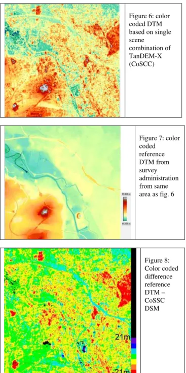
Of course the accuracy specification corresponds to a DSM. The X-band cannot penetrate the vegetation and results in a height approximately 20% of the tree height below the canopy. In addition InSAR is affected by radar layover (fig. 2), causing problems in built up areas and steep mountains. The layover effect is reduced by viewing at least from two different directions and the difficult mountain areas are imaged at least four times also with different inclination angle. In Sörgel et al. 2013 a TanDEM-X InSAR combination has been investigated in the city area of Hannover (fig. 6 and 7).
The difference of both height models (figure 8) shows the influence of buildings and forest (upper right hand side and bigger spots on left hand side). In the inner city area with the TanDEM-X height model the street level mostly cannot be reached, causing some not existing building blocks. With just one InSAR-combination, instead of the average of two combinations used at least for the TanDEM-X final height model, a standard deviation of open areas of 2.07m has been reached with the commercial software ENVE SARscape.
Figure 6: color coded DTM based on single scene
combination of TanDEM-X (CoSCC)
Figure 7: color coded reference DTM from survey administration from same area as fig. 6
Figure 8: Color coded difference reference DTM – CoSSC DSM
4. BATHYMETRIC INFORMATION
Nautical maps up to now are dominated by classical survey by ultra sound, but first tendencies show some changes for shallow water. One reason is the time consuming survey and the requirement for frequent update.
Bathymetric information in shallow water can be determined also based on remote sensing. Bathymetric LiDAR is becoming a common method. In addition with aerial and satellite images a depth determination is possible. With wave structures also water depth can be determined or the width of other measurements can be supplemented.
The first bathymetric LiDAR was developed by Optech for Canadian Hydrographic Service 1984 and further developed 1994 as SHOALS-200 (actual version SHOALS-3000 / Optech Aquarius). The SHOALS-system operates with green light
(532nm) and with near infrared (1064 nm). Riegl for example has a bathymetric LiDAR just operating with green light, reflecting at the water surface and the ground. Water depth from one up to three Secchi-depth (visibility depth of a black/white plate in the water) can be reached depending on the used system and corresponding point spacing.
Within a test project of the German BSH by a HawkEye Mk II airborne Bathymetric LiDAR System the capacity of this system was checked against echo sound depth measurements in the Baltic Sea. In the test area the deepest part of -14.7m was reached with satisfying point density.
Figure 9: discrepancies between bathymetric LiDAR and ultra sound reference
As shown in figure 9 satisfying results have been achieved. Depending upon the water depth up to 14.7m root mean square differences between 10cm for shallow water and 23cm for the deeper water have been reached. Only in a small part, shown in figure 9 in red, up to 60cm discrepancies occurred, caused by sea grass for which the LiDAR pulse went down to the sea floor while the echo sound was set to register the upper part of the sea grass. The overall results have been satisfying, allowing to use LiDAR as a standard method for water depth measurement. In another test by aerial and spaceborne stereo models the water depth has been determined. The aerial measurements reached down to 4m up to 5m depth depending upon the brightness of the seafloor with a standard deviation of 50cm with aerial images guaranteeing on land a standard deviation of the height of 25cm. This has to be multiplied with the effect of the water refraction of approximately 1.4, corresponding to 35cm. A test with IKONOS-images was not very successful because of sun-glitter. Sun-glitter can be avoided if the view direction is directed into the West direction because at 10:30 o clock in the morning the sun is located in South-East direction.
Pleskashevsky and Lehner 2012 are reporting about the use of wave structures available in SAR- or optical images for the determination of the water depth. With homogenous waves, not disturbed by breaking waves, depth information up to 50m can be determined.
5. CONCLUSION
A group of large area covering height models is available today. They are partially even more precise as height models from survey departments in some countries. Not in all countries the height models can be used outside the administration requiring some alternatives. In some other countries the height models can be used but they are too expensive. The SRTM DSM and some derivatives are in frequent use. With ASTER GDEM2 more morphologic details are available, but the accuracy is not better as for SRTM, and also the derivative ACE2 GDEM. Commercial height models as from SPOT 5 HRS, Cartosat-1 and NextMap are an alternative, but with more details and higher accuracy the price is raising. The coming worldwide DSM from TanDEM-X presents a new level of details and accuracy being a real alternative to height models from survey administration. It will be distributed by Airbus Defence and Space (former ASTRIUM).
For nautical maps some changes of the time consuming ultra sound depth measurements are coming, but up to now these are just developing aspects.
6. REFERENCES
Bartusch,M., Miller,D., Zink, M.: TanDEM-X: Mission Overview and Status, http://elib.dlr.de/65150/1/Mission-Overview.pdf
Baudoin, A., Schroeder, M., Valorge, C., Bernard, M., Rudowski, V., 2004: A scientific assessment of the High Resolution Stereoscopic instrument on board of SPOT 5 by ISPRS investigators, ISPRS Congress, Istanbul 2004, Int. Archive of the ISPRS, Vol XXXV, B1, Com1, pp 372-378, http://www.isprs.org/publications/archives.aspx
Danielson, J., Gesch, D., 2011: Global Multi-resolution Terrain Elevation Data 2010 (GMTED2010), http://pubs.usgs.gov/of/2011/1073/pdf/of2011-1073.pdf
Höhle, J., Höhle, M., 2009. Accuracy assessment of digital elevation models by means of robust statistical methods, ISPRS Journal of Photogrammetry and Remote Sensing, 64, pp. 398-406
Jacobsen, K., 2004: DEM Generation by SPOT HRS, ISPRS Congress, Istanbul 2004, Int. Archive of the ISPRS, Vol XXXV, B1, Com1, pp 439-444
Jacobsen K., 2006: ISPRS-ISRO Cartosat-1 Scientific Assessment Programme (C-SAP) Technical report - test areas Mausanne and Warsaw, ISPRS Com IV, Goa 2006, IAPRS Vol. 36 Part 4, pp. 1052-1056
Jacobsen, K., Passini. R., 2010: Analysis of ASTER GDEM Elevation Models, ISPRS Com 1, Calgary 2010, IntArchPhRS. Vol XXXVIII part 1
Jacobsen, K., 2013: Characteristics of Worldwide and nearly Worldwide Height Models, ISPRS WG IV/2 Workshop Interexpo GEO-Siberia-2013, Novosibirsk, proceedings pp 42-57
JCGM 100:2008 : Evaluation of measurement data – Guide to the expression of uncertainty in measurement, http://www.bipm.org/utils/common/documents/jcgm/JCGM_10 0_2008_E.pdf
Passini, R., Betzner, D., Jacobsen, K., 2002: Filtering of Digital Elevation Models, ASPRS annual convention, Washington 2002
Pleskashevsky, A, Lehner, S., 2012: Synergy and Fusion of Synthetic Aperture Radar and Optical Satellite Data for Underwater Topography Estimation in Coastal Areas, SEASAR2012, Tromsö,
Sörgel, U., Jacobsen, K., Schack, L., 2013: TanDEM-X Mission: Overview and Evaluation of intermediate Results, Photogrammetric Weeks 2013
Smith, R.G., Berry, P., 2011: Evaluation of the differences between the SRTM and satellite radar altimetry height measurements and the approach taken for the ACE2 GDEM in areas of large disagreement, J. Environ. Monit., 2011, 13, pp 1646-1652
Tetshshi, T., et al., 2011: ASTER Global Digital Elevation Model Version 2 – Summary of Validation Results, http://www.ersdac.or.jp/GDEM/ver2Validation/Summary_GDE M2_validation_report_final.pdf
Wessel, B., Fritz, T. Eineder, M., Krieger, G., Schättler, B., Zink, M., 2010: TanDEM-X, Ground Segment, DEM Products Specification Document, DFD – German Remote Sensing Data Center, DLR 2010