www.earth-syst-dynam.net/7/313/2016/ doi:10.5194/esd-7-313-2016
© Author(s) 2016. CC Attribution 3.0 License.
Early warning signals of tipping points in
periodically forced systems
Mark S. Williamson1, Sebastian Bathiany2, and Timothy M. Lenton1
1Earth System Science group, College of Life and Environmental Sciences, University of Exeter,
Laver Building, North Park Road, Exeter EX4 4QE, UK
2Aquatic Ecology and Water Quality Management, Wageningen University, PO Box 47,
Wageningen, the Netherlands
Correspondence to:Mark S. Williamson ([email protected])
Received: 27 October 2015 – Published in Earth Syst. Dynam. Discuss.: 6 November 2015 Revised: 4 February 2016 – Accepted: 26 March 2016 – Published: 13 April 2016
Abstract. The prospect of finding generic early warning signals of an approaching tipping point in a complex system has generated much interest recently. Existing methods are predicated on a separation of timescales between the system studied and its forcing. However, many systems, including several candidate tipping elements in the climate system, are forced periodically at a timescale comparable to their internal dynamics. Here we use alternative early warning signals of tipping points due to local bifurcations in systems subjected to periodic forcing whose timescale is similar to the period of the forcing. These systems are not in, or close to, a fixed point. Instead their steady state is described by a periodic attractor. For these systems, phase lag and amplification of the system response can provide early warning signals, based on a linear dynamics approximation. Furthermore, the Fourier spectrum of the system’s time series reveals harmonics of the forcing period in the system response whose amplitude is related to how nonlinear the system’s response is becoming with nonlinear effects becoming more prominent closer to a bifurcation. We apply these indicators as well as a return map analysis to a simple conceptual system and satellite observations of Arctic sea ice area, the latter conjectured to have a bifurcation type tipping point. We find no detectable signal of the Arctic sea ice approaching a local bifurcation.
1 Introduction
The potential for early warning of an approaching abrupt change or “tipping point” in a complex, dynamical sys-tem has been the focus of much research, see for example Wiesenfeld (1985), Held and Kleinen (2004), Thompson and Sieber (2011) and Scheffer et al. (2012). Abrupt change in a system can occur due to a bifurcation – that is, a small smooth change in parameter values can result in a sudden or topological change in the system’s attractors. This extreme sensitivity of systems close to criticality is familiar from studies of critical phenomena in statistical mechanics (Domb et al., 1972–2001) and stability analysis in nonlinear dynam-ical systems (Kuznetsov, 2004). Much work on the anticipa-tion of bifurcaanticipa-tions from time series data, e.g. in ecosystems (Carpenter et al., 2011), or the climate system (Dakos et al., 2008; Lenton, 2011), is based on methods that infer the time
time series. An increasing trend in autocorrelation shows the stability of the system is weakening or equivalently, the sys-tem’s timescale is increasing – which is a generic feature of a system approaching a local bifurcation. Provided the vari-ance of the fast noisy process is constant, increasing varivari-ance of the system’s time series is also a good indicator of critical slowing down, although it is less robust than lag 1 autocorre-lation due to its dependence on the noisy process.
For many systems of interest one or more of the above as-sumptions may be invalid (Williamson and Lenton, 2015). In particular, when the forcing of a system has a comparable period to the timescale of the system, the forcing cannot be modelled as a slow, constant control parameter or a fast, ran-dom process; however they can still be thought of as a pertur-bation away from the system steady state that one can mea-sure the recovery time from, an observation we exploit in this manuscript. These systems are particularly relevant in the cli-mate system where periodic forcing is a consequence of the motion of the Earth relative to the Sun; for example, solar insolation variation from the diurnal, annual or Milankovich cycles. These systems have steady states described by peri-odic attractors rather than the simpler, fixed point type attrac-tors required for lag 1 autocorrelation and variance to be used as early warning indicators.
In an elegant study Wiesenfeld (1985) computed the Fourier spectra of noisy perturbations in systems with peri-odic attractors. Very close to a local bifurcation, the dominant system timescale asymptotes towards infinity causing the dy-namics of the noisy perturbations away from the attractor to be dependent only on the type of bifurcation and not on the details of the system’s specific equations. This observation allowed the author to classify all codimension 1 bifurcations in an arbitrary periodic system by the harmonics in the spec-tra of residuals. He called these early warning signals noisy precursors.
A common method to study stability changes in periodic attractors is the return or Poincaré map, see Strogatz (2001). Here, one converts the continuous-time periodic orbit into the fixed point of a return map by sampling the orbit once every period. One can then compute the usual fixed point in-dicators for the resulting return map time series such as lag 1 autocorrelation and variance. Advantages of this approach include no linearity requirement on the dynamics of the peri-odic attractor although perturbations away from the attractor must be small enough to be treated linearly. One can also handle systems with internally generated cycles rather than those generated by external periodic forcing that we look at in this manuscript. To detect any change in stability from the return map, the timescale of the system must also be greater than the period of the forcing. To see this, imagine one sam-ples the cycle to create a point in the return map and then immediately after perturbs the system away from the stable cycle. If the system timescale is shorter than the cycle pe-riod, which is determined by the forcing pepe-riod, the system will have recovered back to the stable cycle before the
sys-tem is sampled again for the next point in the return map. The perturbation and its recovery will therefore be invisible to stability analysis on the return map time series. It should be noted that close to a local bifurcation the system timescale approaches infinity so satisfying this requirement. However, if this requirement is met only over a few cycles or less it will be very hard to detect.
With this limitation in mind we suggest alternative early warning signals of approaching local bifurcations when the period of the forcing is similar to the timescale of the sys-tem. We look particularly at sinusoidal forcing since this ap-proximates the variation of solar insolation well. However, the method works for any periodic forcing and we give the derivation of the general case in the Appendix. We demon-strate that increasing the system timescale as it approaches a local bifurcation shows up as an increasing phase lag in the system response relative to the forcing. In addition, the amplitude of the system response increases as well. These indicators, like lag 1 autocorrelation and variance in fixed point attractor methods, assume the linearised dynamics ap-proximate the true nonlinear dynamics well. One might ask how well the linear approximation works, especially near the bifurcation, since bifurcations are strictly nonlinear phenom-ena. A quantitative answer to this question can be provided by computing the Fourier spectrum of the system’s time se-ries. In particular, as the system’s behaviour becomes more nonlinear, harmonics of the forcing period are generated in the system response and their amplitudes may be obtained from the system’s Fourier spectra. Since the system response becomes more nonlinear as one approaches the bifurcation, one can view the increasing amplitude of harmonics as an-other early warning signal.
The paper is organised as follows: in Sect. 2 the early warning indicators used in the manuscript are introduced, namely the system response phase lag and amplification as well as harmonic amplitudes. We also review a common approach to periodic attractors, the return map, which is complementary to phase lag and response amplification. In Sect. 3 a periodically forced overdamped system in a double well potential is used to illustrate the timescale separation problem and the properties of the early warning indicators when a local bifurcation is approached. In Sect. 4 we apply the early warning indicators to satellite observations of Arc-tic sea ice area, a system conjectured to be approaching a local bifurcation. We conclude in Sect. 5.
2 Early warning indicators of local bifurcations in periodic systems
temperature as the Earth’s atmospheric CO2 concentration
increases. This is a system that is forced periodically and de-terministically by the annual cycle of short-wave solar in-solation. The system response is dominated by this periodic forcing rather than small amplitude; random noisy forcing is also present and system timescale is roughly the same order of the forcing period. In this section, motivated by detection of local bifurcations in systems like the sea-ice type from time series, we look for suitable methods. Although this sys-tem has no clear separation of timescales with which to use fixed point methods directly, the fact that this system has a large and predictable perturbation one can measure the re-sponse to reduces the need for the statistical methods (and therefore large numbers of data) required for noisy perturba-tions and so the number of data in a time series becomes less of an issue.
Students of physics or engineering will likely have solved the equation for the forced damped harmonic oscillator and observed in the overdamped limit that the phase and am-plitude depend on the damping parameter (see for example Main, 1993). In the following subsections we propose to use this fact and phase lag and response amplification as sim-ple non-statistical indicators of system timescale. We demon-strate their properties and their functional dependence on sys-tem timescale. These early warnings are based on a linear dy-namics approximation but by taking the Fourier transform of the system response, one can also look at the magnitude of the nonlinear response. This has two purposes, first one can check the linear approximation is good and second, because bifurcations are strictly nonlinear phenomena, the system re-sponse will become more nonlinear as one approaches the bifurcation giving another early warning indicator that can be monitored.
The systems we concentrate on in this manuscript, relevant to externally forced climate problems, have cycle periods de-termined by the period of forcing and a one-way coupling from the forcing to the system and so are special cases of pe-riodic attractors. For these special cases, when forcing period and system timescale are similar, phase lag and response am-plification are useful indicators. However, return maps are generally more useful when treating more general periodic attractors. At the end of the section we briefly review the method of return maps.
2.1 Phase lag and response amplification We consider systems that can be described by
˙
x=f(x)+D(t) (1)
wheref(x) is, generally, a nonlinear function of the system state scalar variablexwith forcingD(t) given by
D(t)=Dm+Dacos(ωt). (2)
Dm andDa are constants,ω=2Tπ is the angular frequency and T is the period of the forcing. We have assumed any
other random, noisy external forcing to be very small and can be neglected. The solution for a general form forD(t) is given in the Appendix, however here we use sinusoidal forcing as this is most relevant for many climate systems and we wish not to obscure the simplicity of the main result.x˙
describes the dynamics of a forced overdamped system. This is a nonautonomous system whose state can be completely described byt and x. After some time ts≫τ, whereτ is the system timescale, the system will settle into some sort of steady state, either an orbit or a fixed point whose mean state
¯
xis
¯
x= 1 T
T+ts Z
ts
x(t)dt. (3)
We now Taylor expandf(x) to first order aroundx¯so that
˙
x≈a−x
τ +Dacos(ωt), (4)
where
a=f(x)¯ −∂f
∂x|x= ¯xx¯+Dm (5)
τ= −1/∂f
∂x|x= ¯x (6)
are the linearisation constants. We have assumed higher order terms such asn1!∂∂xnfn(x− ¯x)n,n≥2 are small relative to zeroth
and first order terms so that the linearised dynamics approx-imates the full nonlinear dynamics well. We show how to check this approximation in Sect. 2.2. Assuming the approx-imation is good, one can solve Eq. (4). Ast≫τ the system settles into the orbit
lim
t≫τx(t)=aτ+ Daτ √
1+ω2τ2cos(ωt+φ), (7)
where the system response lags the forcing by phaseφlag=
ωtlag= −φgiven by
φlag=arctan(ωτ), (8)
that is, the phase lag is a function of the forcing frequency and the system response timescale. One also notices that the system response, relative to the forcing amplitude,Da, is am-plified by a factor
τ
√
1+ω2τ2, (9)
which is also a direct function ofωandτ. The more general derivation whenD(t) can be any periodic function is given in the Appendix Sect. A.
2.2 System nonlinearity and harmonic amplitude from Fourier analysis
phase lag are when the driving is of the form Eq. (2) and the system response is approximately linear without the need for statistics. However, the system is essentially nonlinear and these nonlinear effects may become large near a bifurca-tion or when the system is driven hard. By taking the Fourier transform of the time series of the system response one can quantify how large these nonlinear effects are. With a simi-lar motivation Wiesenfeld (1985) and Wiesenfeld and McNa-mara (1986) calculated the Fourier spectra of the perturba-tions, rather than the response, away from periodic attractors very close to local bifurcations with noisy and weak periodic modulation respectively.
Once the system has settled into an orbit of periodT, the full nonlinear response of an arbitrary system can be written as a Fourier series, a sum ofN sinusoidal functions with an-gular frequenciesωn=2π nT , amplitudesAn and phasesφn, i.e.
x(t)= N
X
n=0
Ancos(ωnt+φn). (10)
The n=0 component is a constant, the long-term mean of the response; then=1 component is the linear response of the system and then≥2 components are thenth order har-monics and come about from the nonlinear response of the system. Since the system has settled into a periodic orbit the system must repeat itself every cycle. The only way the sys-tem can do this is by adding harmonics to linear response. By looking at the ratios An/A1 for n≥2 the nonlinear
ef-fects relative to the linear approximation can be quantified. In practice the largest harmonics will generally be the 2nd (n=2) and 3rd order (n=3) harmonics and provided they are an order of magnitude (10 times, An/A1<10−1) less
than the fundamental harmonic, the linear analysis in the last section works well. Calculation of the amplitudes,An, can be made via a Fourier transform of the time series.
One may also expect subharmonics, components that have periods that are integer multiples of the forcing period, to be observed in the system response. Subharmonics are not possible in the systems we consider here due to the dimen-sionality of the phase space.1
Since the ratiosAn/A1measure how nonlinear the system
is one expects these to increase as the system approaches a
1Systems described by Eq. (1) are completely described by the
two-dimensional space of variablesxandt. Recasting the nonau-tonomous system in Eq. (1) as a two dimensional aunonau-tonomous sys-tem by identifying a new angular variable φ=ωt, the system is then described byx˙=f(x)+D(φ) andφ˙=ω. The resulting phase space (x, φ) is then cylindrical asφis 2π modular. If subharmon-ics are possible in the periodic system response the trajectory must wind around the cylinder at least twice before repeating itself. Such a trajectory implies it crosses itself which is not allowed due to the existence and uniqueness theorem. Therefore subharmonics cannot exist in the two-dimensional systems. This is of course not true for three- and higher-dimensional systems.
bifurcation. These ratios can be plotted for a time series by taking the Fourier transform for a data window consisting of an integer number of cycles and sliding this window forward by one cycle recursively through the time series. The number of cycles in the window must be large enough that the har-monics can be satisfactorily resolved in the Fourier spectra. In addition, each cycle must be sampled at a time interval 1t≤TNyquist/2 whereTNyquistis the minimum harmonic
pe-riod you want to resolve.
2.3 Lag 1 autocorrelation of a return map
Provided the system timescale is larger than its period, τ/T >1, one can use return maps to assess the stability of a periodic attractor. The return map time series, generated by sampling the system response once every cycle, allows one to apply fixed point statistical early warning indicators such as lag 1 autocorrelation. It is the random forcing away from the periodic attractor that this method infers timescale from, rather than response to deterministic, periodic forcing. This is usually done by calculating the lag 1 autocorrelation for a sliding data window of the return map time series at least as long as the system timescale but not so long that any in-creasing trend in system timescale skews the autocorrelation estimate. It is also desirable to have many points within this window as the standard error of the estimate scales as 1/√m, wheremis the number of cycles (points) within the window (see Williamson and Lenton (2015) for a discussion). For time series consisting of a small number of cycles this can be a limiting factor.
3 Examples
We now demonstrate the early warning indicators in Sect. 2 for different ratios of forcing period,T, (or equivalently an-gular frequencyω) to system timescaleτ. In particular, we use a periodically forced double well potential as our main system. This system has been extensively studied in the con-text of stochastic resonance (see McNamara and Wiesenfeld (1989) and Gammaitoni et al. (1998) for reviews) as the sim-plest model of the phenomena when noise is also added. Phase and amplitude have been investigated in this setting by Shneidman et al. (1994) and Jung and Hänggi (1993). This literature is largely concerned with resonance effects in tran-sition probabilities between the wells (finite barrier height between the wells) rather than the anticipation of local bifur-cations (barrier height tends to zero).
Our system which has one dynamical variable, x, and evolves according to
˙
x=x−x3+D(t), (11)
the overdamped limit of a Duffing oscillator (Thompson and Stewart, 2002). When forcing is constant (ω=0) the famil-iar, well-studied autonomous fold bifurcation is recovered (for example see Strogatz, 2001). For ω=0, the solutions of x˙=0, give the system’s fixed points,x∗ (the nullclines) and number either one or three depending on the value of Dm. One can evaluate the stability of these fixed points by looking at the linearised dynamics close to the fixed points, J(x∗):
J(x∗)=∂x˙
∂x|x=x∗=1−3x
∗2.
(12)
IfJ(x∗) is negative, the fixed point is stable, if it is positive it is unstable. In the region where three fixed points exist one finds a bistable region, i.e. two points are stable while the third is unstable. The bistable region has boundaries marked by the local bifurcations and these can be found by solving J(x∗)=0 forx∗when the fixed point becomes neutrally sta-ble. One can also calculate thee-folding timescale of the sys-tem in statex,τ from the Jacobianτ = −1/J(x). We will re-fer to thee-folding time as the system timescale. As the sys-tem gets closer to the bifurcation the syssys-tem timescale will increase and tend to infinity at the bifurcation. Early warning indicators are simply functions ofJ(x∗) or equivalentlyτ.
3.1 Period of forcing similar to system timescale,ωτ∼1
This regime, T ∼τ, is the main focus study in this manuscript, when the system responds on approximately the same timescale as the period of the forcing. In this regime the dynamics are a balance between the system’s tendency to want to decay towards the fixed point and the forcing try-ing to push it away. After some time,t≫τ, the system will settle into an orbit rather than a fixed point due to the sim-ilarity of the timescales. Just as there was a bistable region where multiple stable fixed points existed for a single value ofDmwhenω=0, analogously in the caseT ∼τ multiple stable periodic attractors are possible given a fixed set of val-ues forDm,Daandω. The system statex is plotted against Dand againsttas the blue line in Fig. 1. Which state the sys-tem settles in depends only on the syssys-tem’s initial condition x(t=0). Local bifurcations are present in this intermediate region, however they are local bifurcations between orbits rather than fixed points. In this intermediate regime, one can neither place theDacos(ωt) part of D(t) in either the slow or fast processes and therefore the assumptions of the usual fixed point early warning methods are not strictly valid. This is, however, where phase lag and response amplification are useful early warning indicators.
To illustrate the early warning indicators we fix the forc-ing amplitude Da and the period T ∼O(τ) and take Dm as a control parameter, slowly varying from negative val-ues towards the local bifurcation in the system described by Eq. (11). We expect to see the system response become more phase lagged and amplified as we approach the local
bifur-−1 −0.8 −0.6 −0.4 −0.2 0 0.2 0.4 0.6 0.8 1
−1.5 −1 −0.5 0 0.5 1 1.5
(a)
D
x
0 0.2 0.4 0.6 0.8 1 1.2 1.4 1.6 1.8 2
−1.5 −1 −0.5 0 0.5 1 1.5
t/T
x
(b)
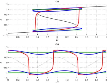
Figure 1.The dynamics of the system described by Eq. (11) in three
different timescale regimes. Forcing parameters are set toDm=0,
Da=1/2. In the upper panel system statexis plotted againstD(t). The black lines are the nullclines and the coloured lines are the sys-tem responses for different periods of forcing. In the lower panelx
is plotted against the number of cycles,t /T, once the system has reached a steady state. The dotted line is the forcing,D(t) while the coloured lines are the system responses. The red line is for the slow forcing limit,τ≪T,T =100πsoωτ≈1/100. As the sys-tem timescale is much faster than the change in the forcing, the system essentially “sticks” to the fixed points until they become unstable at the bifurcations and jump to a different attractor. One can regard the system response in two different ways: (i) a single periodic attractor giving relaxation oscillations in a monostable re-gion. (ii) Tipping between point attractors by crossing local bifur-cations in a bistable region. This tipping causes the dynamics to be very nonlinear. The green line is the fast forcing limit,T ≪τ,
T=π/100 soωτ≈100. There are two possible stable attractors for this set of values. As the system timescale is much slower than the change in the forcing, the system essentially remains static and all the dynamics come from the forcing itself. Although it is hard to see in the figure due to the small amplitude system response, the lag relative to the forcing is 1/4 of a cycle and the dynamics are ap-proximately linear. The blue line is the intermediate regime,τ∼T,
T=πsoωτ≈1 and there are two possible stable attractors for this set of values. As the system timescale is approximately the same as the period of the forcing, the system response is a competition be-tween the system’s tendency to decay towards the nullcline and the forcing pushing it away setting up a stable orbit. Notice that there is some phase lag and the dynamics look approximately linear.
cation atDm≈0.33 when approaching from the lower null-cline solutions. We also expect the amplitude of the harmon-ics of the system response to increase.
−2 −1.5 −1 −0.5 0 0.5 1 1.5 2 −2
−1 0 1 2
(a)
D
x
0 5 10 15 20 25
−2 −1 0 1 2
t/T
x
(b)
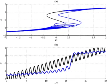
Figure 2.The dynamics of the system are described by Eq. (11)
with varyingDm. Parameters are set toDa=1/2,T=π(the same order as the system timescale ωτ∼1) andDm is varied linearly with time between -2 and 2 over about 25 cycles. In the upper panel the black lines are the nullclines while the system response is the blue line plotted against D(t). The orbit loses stability around a mean value ofD≈0.5 and jumps to a new orbit. In the lower panel we have plotted the system response (blue) against the forcingD
againstt /T. One can see the loss of stability of the orbit around
t /T ≈15 and the prior increase in system response amplitude.
phase lag depends onω, one must take this into account when inferring system timescales from the indicators.
In Fig. 2 the system is run forward in time, linearly vary-ing Dm from−2 to 2 across the bifurcation over about 25 cycles of the forcing period (for the values of the parame-ters see the figure caption). Plotted in Fig. 3 are phase lag and amplitude of the system response prior to the bifurcation at aroundt /T =15. Both are increasing as the bifurcation is approached due to the increase in τ. Phase lag is calcu-lated from the difference between the times of the maxima in the forcing and the system response in each cycle. Re-sponse amplitude is calculated by taking half the difference between the maximal and minimal values in the system re-sponse in each cycle. Also plotted are the ratios of the sec-ond and third harmonic amplitudes to the amplitude of the fundamental harmonic with time using a sliding window of length 5 complete cycles against the time at the end of the sliding window. The window needs to be long enough to re-solve the harmonics in the spectrum but short enough to keep Dmapproximately constant. For this example, where the har-monic amplitudes (and the nonlinearity of the response) are quite small, 5 cycles is the minimum to resolve the peaks. The sliding window is then advanced one cycle in the time series and the harmonic amplitudes are calculated for this new window. This process is iterated until the local bifurca-tion is reached to produce the lower panel in Fig. 3 which shows both harmonic amplitudes increasing.
0 5 10 15
0 0.1 0.2
A
(a)
0 5 10 15
0 0.1 0.2
φlag
/2
π
(b)
0 5 10 15
0 0.01 0.02 0.03
t/T An
/A
1
(c)
Figure 3.The early warning indicators, response amplification
(up-per panel),A= √Daτ
1+ω2τ2, and phase lag (middle panel),
φlag 2π =
1
2πarctan(ωτ) calculated for the time series in Fig. 2. We have plot-ted these indicators prior to the bifurcation att /T ≈15. The 2nd (blue) and 3rd (red) harmonic amplitudesAn/A1are also plotted in
the lower panel using a sliding window of 5 complete cycles. All indicators are increasing as expected.
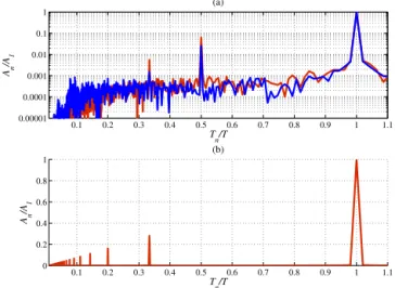
We also plot the complete spectrum of the ratiosAn/A1
againstTn/T derived from a Fourier transform of the sys-tem response in Fig. 4. In the upper panel all parameters are the same as Fig. 2 except we have fixedDm in each of the two runs. In the first runDm= −2, this is far from the bi-furcation and one expects the system to behave more linearly (blue line). One sees a second harmonic around 2 orders of magnitude smaller than the linear response. In the second run Dm=0.25 and the orbit is much closer to the bifurcation (red line). The second harmonic has increased to about an order of magnitude smaller than the fundamental harmonic and a third harmonic is now also visible indicating the system has become more nonlinear.
To give an example of a climate system operating in this regime consider the annual variation in sea temperatures in Northern Hemisphere temperate regions. A rough estimate of the ocean surface mixed layer timescale givesτ ∼10 months and this surface layer is heated by the annual cycle of solar insolation to varying degrees throughout the year. Calcula-tion of the phase lag for thisτ andT yields a lag of about 2.6 months, i.e. roughly the maximal and minimal sea tem-peratures are in September and March. Arctic sea ice ex-tent also falls into this regime and we analyse this system in Sect. 4.
3.1.1 A note about return maps
0.1 0.2 0.3 0.4 0.5 0.6 0.7 0.8 0.9 1 1.1 0.00001
0.0001 0.001 0.01 0.1 1
T
n/T
An
/A1
(a)
0.1 0.2 0.3 0.4 0.5 0.6 0.7 0.8 0.9 1 1.1
0 0.2 0.4 0.6 0.8 1
T
n/T
An
/A
1
(b)
Figure 4.Ratio of thenth order harmonic amplitude to the
fun-damental harmonic amplitudeAn/A1against the ratio of thenth
harmonic period to the fundamental harmonic periodTn/T. The dynamics of the system are described by equation 11. In the up-per panel parameters are fixed toDa=1/2,T=π (the same or-der as the system timescaleτ). The blue line is forDm= −2 (far away from the bifurcation), the nonlinear response is dominated by the second harmonic atTn/T=1/2 although small, about two orders of magnitude less than the linear response. The red line is
Dm=1/4, close to the bifurcation the system response has be-come more nonlinear. The second harmonic (Tn/T=1/2) is now almost 1 order of magnitude less and the third order harmonic (Tn/T=1/3) is also prominent. In the bottom panel, we show the spectrum when the dynamics are very nonlinear. Parameters are set toDm=0,Da=1/2,T =100π soωτ≈1/100. This is the slow forcing limit shown in Fig. 1 (red line) which has a very nonlin-ear relaxation oscillation type response. Note only odd harmonics (Tn/T=1/3,1/5,1/7, . . .etc.) are present due to the system expe-riencing a symmetric potential requiring the solution,x(t), to also have this symmetry.
the system must have enough cycles to produce statistically significant results. Return map analysis is complementary to phase lag and response amplification since these quantities start to asymptote whenωτ >2π. This complementarity is illustrated in the following figures. The blue line in Fig. 5 is essentially the same as Fig. 2 (ωτ∼1) exceptDmis var-ied over 100 cycles instead of 25. This is because extra data points are needed to calculate the lag 1 autocorrelation of the return maps with any reliability. We have also added Gaus-sian white noise to Eq. (11) of standard deviation 0.01 as the return map method needs small perturbations with which to infer return times to the cycle. In Fig. 6 we have plotted the early warning indicators for this time series including the re-turn map calculated with a sliding window of 25 cycles. The black lines are the theoretical curves and the blue lines are the estimated curves. The key point is the theory and esti-mated autocorrelations do not show anything in this regime (ωτ∼1) however the phase lag and response amplification are clearly increasing.
−2 −1.5 −1 −0.5 0 0.5 1 1.5 2
−2 −1 0 1 2
D
x
0 10 20 30 40 50 60 70 80 90 100
−2 −1 0 1 2
x
t/T
0 10 20 30 40 50 60 70 80 90 100−4
−2 0 2 4
D
Figure 5.Same figure as Fig. 2 in the manuscript except the
varia-tion ofDmis over more cycles to generate more points for a reliable return map analysis. Weak Gaussian white noise of standard devia-tion 0.01 is added to the system. Parameters are set toDa=1/2 and
Dmis varied linearly with time between−2 and 2 over about 100 cycles. In the upper panel the black lines are the nullclines while the system response is the blue line forT =πgivingωτ∼1 whereas the red line has a shorter period ofT =1/4 to giveωτ∼4π. These are plotted againstD(t). In the lower panel we have plotted these system responses as time series against the forcing (black line).
Conversely, the red lines in Figs. 5 and 7 are the same quantities but with a decreased period of forcing (T =1/4 so ωτ∼4π). This is a regime in which phase lag and response amplitude start to asymptote and are therefore not so useful to infer changing system timescale. However, lag 1 autocor-relation of the return map now becomes useful as can be seen in Fig. 7.
3.2 Period of forcing much slower than system timescale,ωτ≪1
When Eq. (11) is operating in this regime (period of forcing much greater than system timescaleT ≫τ) the system can adjust to changingD(t) relatively quickly and effectively re-mains at a fixed point.D(t) can therefore be modelled as a slow constant, control parameter and all the usual timescale separation assumptions apply. Fixed point indicators such as lag 1 autocorrelation are then good early warning indi-cators of local bifurcations. In contrast, phase lag and re-sponse amplitude are not useful as these quantities asymp-tote toφlag→0 and→τ respectively. The system statexis
superpo-0 10 20 30 40 50 60 70 80 90 100 0
0.1 0.2
A
0 10 20 30 40 50 60 70 80 90 100
0 0.1 0.2 0.3
φlag
/2
π
0 10 20 30 40 50 60 70 80 90 100
−0.5 0 0.5
t/T
AR(1)
Figure 6.ωτ∼1: The early warning indicators, response
amplifi-cation (upper panel),A=√Daτ
1+ω2τ2, and phase lag (middle panel),
φlag 2π =
1
2πarctan(ωτ) calculated for the blue time series in Fig. 5. In the lower panel, lag 1 autocorrelation of a sliding window of 25 points of the return map is plotted with standard errors (dashed lines) on the estimate. Black lines are theoretical curves of all the quantities. The key point is that phase lag and amplitude response are useful quantities in this regime however the return map is not.
sition of many different sinusoidal frequencies, the domi-nant ones having periods of 41 kyr (related to the obliquity of Earth’s orbit), 19 and 23 kyr (related to the precession). Current thinking, however, favours more complex, two- and higher-dimensional dynamics to model these cycles than the single variable models we consider in this paper (Saltzman, 2002; Crucifix, 2012; Saedeleer et al., 2013; Crucifix, 2013). The spectrum of a very nonlinear, relaxation oscillation type, dynamics is illustrated in the lower panel of Fig. 4. This is the spectrum of the slow forcing run (red line) in Fig. 1. Only odd harmonics appear in its spectrum because the static potentialV = −R
˙
xdxis symmetric aboutxfor this value of Dm=0, i.e.V(x)=V(−x) and therefore any solution ofx˙ must also have this symmetry,x(t+T /2)= −x(t). Only odd harmonics have this property.2
2This is not sufficient though as there are other parameter
set-tings that feature the second harmonic and also have the same sym-metric potential, i.e.Dm=0 andT =π in Fig. 1 (blue line). The difference is that the runs featuring second harmonic responses only experience a limited part of the potential, not the full symmetric po-tential. Even though the potential is the same, the forcing is quick enough to trap the system in an orbit in just one of the two potential wells. This local potential well is asymmetric and what the system sees is effectively described by a Taylor expansion around the cen-tre of that well. In contrast the relaxation oscillation type run travels across both wells equally and therefore sees the global symmetric potential requiring an odd harmonic solution. This is not a generic case however.
0 10 20 30 40 50 60 70 80 90 100
0 0.01 0.02
A
0 10 20 30 40 50 60 70 80 90 100
0 0.1 0.2 0.3
φlag
/2
π
10 20 30 40 50 60 70 80 90
0 0.5 1
t/T
AR(1)
Figure 7.ωτ∼4π: The early warning indicators, response
amplifi-cation (upper panel),A=√Daτ
1+ω2τ2, and phase lag (middle panel),
φlag 2π =
1
2πarctan(ωτ) calculated for the red time series in Fig. 5. In the lower panel, lag 1 autocorrelation of a sliding window of 25 points of the return map is plotted with standard errors (dashed lines) on the estimate. Black lines are theoretical curves of all the quantities. Phase lag and amplitude response have now asymptoted and are not useful quantities however the return map now becomes useful.
3.3 Period of forcing much faster than system timescale,
ωτ≫1
The system statex is plotted againstDand againstt as the green line in Fig. 1. The forcing is changing much faster than the system can respond so the system effectively looks static and all the dynamics come from the forcing directly. In this case we can placeD(t) in the fast dynamics. However, not all of the other assumptions for use of lag 1 autocorrelation in a fixed point analysis are satisfied. It is true thatD(t) is independent ofx, however it is not uncorrelated with itself at different times and therefore cannot strictly be modelled as a normally distributed random variable, although at first glance it looks as though it is again possible to use usual fixed point early warning techniques so one must be careful. In this regime, phase lag and response amplification asymptote and again are not very useful to detect a trend in increasing timescale. Phase lag,φlag→π/2 and response amplification
→ω1 so one may only inferτ ≫T.
1975 1980 1985 1990 1995 2000 2005 2010 2015 320
340 360 380 400 420
year
CO
2
(ppm)
(a)
1975 1980 1985 1990 1995 2000 2005 2010 2015
0.65 0.7 0.75 0.8
Year
Time of year of min ann. CO
2 (b)
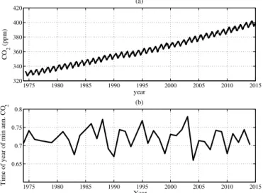
Figure 8.Atmospheric CO2concentration recorded at Mauna Loa
against time in the upper panel. In the lower panel we have plot-ted the minimum annual CO2concentration against year. One
no-tices the minimum CO2concentration occurs roughly 3/4 of the way through the year. This is because maximal carbon uptake oc-curs during the Northern Hemisphere summer from the terrestrial vegetation and it is maximally lagged behind the maximum in the Northern hemisphere solar insolation (best growing conditions) by 1/4 of a cycle because of the timescale difference between the re-sponse of the system and the period of the forcing.
the annual minimum of the Mauna Loa CO2 record3
rela-tive to the Northern Hemisphere solar insolation maximum. This lagged annual minimum in the integrated response of the total atmospheric carbon results from the dominance of the Northern Hemisphere’s mid latitude terrestrial vegetation carbon in the global carbon flux. We have plotted the Mauna Loa CO2 record and the time of year of the minimum
con-centration in Fig. 8.
4 Looking for a tipping point in Arctic sea ice satellite observations
There has been much research on a possible local bifurcation and tipping point in the Arctic sea ice, see for example Ar-mour et al. (2011), Eisenman and Wettlaufer (2009), Lindsay and Zhang (2005), Livina and Lenton (2013), Ridley et al. (2012) and Wang and Overland (2012). This possible bifur-cation in the sea ice cover may be due to the well-known ice albedo feedback first studied by Budyko (1969) and Sell-ers (1969). When ice is present it reflects a high proportion of the incoming solar radiation due to its higher albedo yet when it starts receding the darker ocean absorbs more radi-ation increasing heating and promoting more sea ice retreat.
3Pieter Tans, NOAA/ESRL (www.esrl.noaa.gov/gmd/ccgg/
trends/) and Ralph Keeling, Scripps Institution of Oceanography (www.scrippsco2.ucsd.edu/)
1980 1985 1990 1995 2000 2005 2010 2015
2 4 6 8 10 12 14 16
Year
Sea
ice
area
(10
km
)
6
2
Figure 9.Arctic sea ice area satellite observations from 1979 to
present day (2015) obtained from The Cryosphere Today project of the University of Illinois.
This feedback can result in instability and multiple steady states.
We calculate all the previously mentioned early warning indicators for a time series of Arctic sea ice area satellite observations from 1979 to present day. That is we calcu-late phase lag, response amplitude, relative size of the 2nd and 3rd harmonics and the lag 1 autocorrelation of the return map with time to look for signs of critical slowing down that might indicate the approach of a local bifurcation or “tipping point” in the Arctic sea-ice. We also calculate the complete Fourier spectra for the entire time series as a linearity check. In Fig. 9 satellite observations of Arctic sea ice area are plot-ted against year. Sea ice area data were obtained from The Cryosphere Today project of the University of Illinois. This data set4 uses SSM/I and SMMR series satellite products and spans 1979 to present at daily resolution.
In Fig. 10 we plot the amplitude of the sea ice area annual cycle and the phase lag between the sea ice area minimum and maximum during each cycle. We assume the maximal and minimal driving occurs at the same time as maximal and minimal of the solar insolation, that is, the midpoint and end point of the year respectively to obtain phase lags. To limit the impact of high-frequency variability on the location of the extrema, we have smoothed the daily data with a sliding window of 30 days.
From Fig. 10 we see the cycle amplitude is increas-ing with time although the phase lag does not appreciably change. We first make some rough calculations to see if these plots are consistent with each other: from the phase lag figure, a timescale ofτ ∼[0.33, 0.5] years from the lag of [0.18, 0.2] of a cycle can be inferred. If we assume for the moment the amplitude of the forcingDa is not chang-ing throughout the time period of the observations (this may not be true) and take the smallest value in the range for
4http://arctic.atmos.uiuc.edu/cryosphere/timeseries.anom.
19804 1985 1990 1995 2000 2005 2010 2015 5
6
Amplitude
(10
km
)
6
2 (a)
1980 1985 1990 1995 2000 2005 2010 2015
0.1 0.15 0.2 0.25
φlag
/2
π
(b)
1980 1985 1990 1995 2000 2005 2010 2015
0.12 0.14 0.16
A2
/A1
Year (c)
1980 1985 1990 1995 2000 2005 2010 20150.03
0.035 0.04 0.045
A3
/A1
Figure 10.In the upper panel amplitude of sea ice area within each
cycle is plotted against year. In the middle panel phase lag is plotted between the sea ice area minimum (red line) and maximum (blue line) and the solar insolation minimum and maximum respectively against the year. In the lower panel, the 2nd (blue) and 3rd (red) harmonic amplitudesAn/A1are plotted against year end using a
sliding window of 10 years. The amplitude is increasing however the phase lag is not. Harmonic amplitudes also show no convincing trend.
τ1978=0.33 years occurring in 1978 and the largest value
in 2015,τ2015=0.5 years we can make a rough calculation
of how much the sea ice amplitude would have increased,
i.e. A2015
A1978 =
τ2015
τ1978 r
1+ω2τ2 1978 1+ω2τ
2015 ≈1.06. From Fig. 10 we take
the amplitude at 1978 to be A1978∼4.5 and at 2015 to be
A2015∼5 we findAA2015
1978 =1.11. These values could therefore
be consistent with a constantDa and a changing timescale. However, the timescales inferred from either the phase lag or amplitude are not changing appreciably and therefore it seems unlikely the system is approaching a local bifurcation. We note that the phase lag is a more robust indicator. This is because the phase lag depends only on the product of the frequency of the forcing and the system timescale whereas the amplitude depends additionally on the amplitude of the driving,Da, which may well be changing throughout the ob-servational period and could account for some or all of the increase seen in the amplitude in Fig. 10. Although the solar insolation will be a large component of the forcing amplitude and is essentially fixed, other factors such as clouds as well as air and sea temperatures will also factor into the driving amplitude. Geometrical constraints imposed by land masses affecting the maximal extent of the sea ice will also influ-ence the amplitude of the sea ice oscillation when ice extent is large (Eisenman, 2010). In contrast, we can take the fre-quency of the driving to be essentially fixed by the annual solar insolation cycle making the phase lag more robust.
In the lower panel of Fig. 10 we have plotted the ratio of the second and third harmonic amplitudes to the amplitude of the fundamental harmonic with time using a sliding
win-0.1 0.2 0.3 0.4 0.5 0.6 0.7 0.8 0.9 1 1.1
0.0001 0.001 0.01 0.1 1
T
n/T
An /A1
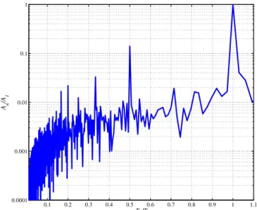
Figure 11.Ratio of thenth order harmonic amplitude to the
fun-damental harmonic amplitudeAn/A1found from the Fourier
trans-form of the Arctic sea ice area time series against the ratio of thenth harmonic period to the fundamental harmonic periodTn/T. One can see the Arctic sea ice response features prominent second, third, forth, fifth and sixth harmonics in its spectrum.
dow of 10 complete cycles against the year at the end of the window. We have used the minimal window length needed to resolve both harmonics reliably. This indicator also shows no clear trend with time.
19980 2002 2006 2010 2014 50
100 150 200 250 300 350
AR(1)
Year
Day of the year
19980 2002 2006 2010 2014
50 100 150 200 250 300 350
Year
Day of the year
Standard error/AR(1)
−0.5 0 0.5 0 0.1 0.2 0.3 0.4 0.5
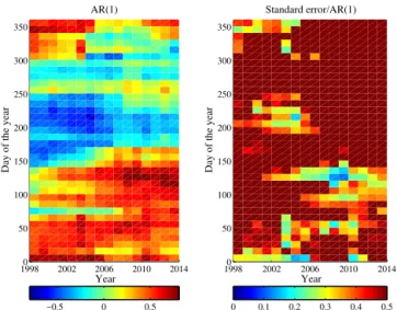
Figure 12. Left panel: Lag 1 autocorrelation of the return map
against sliding window end year using a sliding window of 20 years (xaxis) and point within the cycle the return map is created on the
y axis (we create return maps every 10 days). One sees that auto-correlation depends very heavily on where in the cycle one chooses to generate the return map. Right panel: standard error of the au-tocorrelation return map estimate divided by the estimate against sliding window end year. The estimate is very uncertain almost ev-erywhere with standard errors generally being at least half as big as the estimate.
not changing. In the left hand panel of Fig. 12 we plot the standard error divided by the autocorrelation. Note that most estimates of lag 1 autocorrelation have standard errors larger than half their value giving very uncertain estimates. In an effort to reduce the uncertainty in the estimate we have also taken the mean autocorrelation over all points in the cycle the return map is taken in Fig. 13. The mean lag 1 autocorrela-tion is 0.16±0.26 which corresponds to a (very uncertain) timescale of τ≈0.55 years. This is consistent with the es-timates from the phase lag. This also suggests that the sam-pling intervalT > τand therefore determining the timescale using the return map approach is difficult. We have increased the sliding window to 37 years to minimize the standard er-ror in the estimate, however one will not be able to then see a trend in autocorrelation. Even so, the standard errors are still greater than half the estimate.
We have also plotted the full spectrum of the ratiosAn/A1
for the entire time series in Fig. 11. We note the nonlinear effects are quite prominent in this system, second and third harmonics are around an order of magnitude smaller than the linear response, although we can still probably get away with the linear analysis. Forth, fifth and sixth harmonics are also visible. These nonlinearities may be due to albedo effect or to the geometrical effects of the Arctic ocean basin (Eisenman, 2010).
To conclude, from this simple analysis it seems that the system’s timescale and therefore stability is not changing
1998 2000 2002 2004 2006 2008 2010 2012 2014
−0.2 −0.1 0 0.1 0.2 0.3 0.4 0.5 0.6
Year
Mean AR(1)
Figure 13.Mean lag 1 autocorrelation of the return map across all
starting points within the cycle using a sliding window of 20 years. This is the same as Fig. 12 with the mean taken along theyaxis. Estimated autocorrelation is still very uncertain. The mean is the solid line with the dotted lines being the mean plus or minus the standard error. The mean value across all years 0.16±0.26 which corresponds to a (very uncertain) timescale ofτ≈0.55 years.
appreciably if at all and it is unlikely to be approaching a local bifurcation. However, simple theoretical models, such as Eisenman and Wettlaufer (2009), Eisenman (2012) and Bathiany et al. (2016, who also used a return map approach) suggest that the sea ice timescale does not change very much approaching the bifurcation, even decreasing slightly before rapidly changing over a very small interval and therefore would be very hard to detect if present.
5 Conclusions
and response amplification respectively. Just as autocorrela-tion is more robust as an indicator (it is a funcautocorrela-tion of fewer parameters), the same is true of phase lag, only depending on the frequency of the forcing and the timescale of the system. The system response amplification also depends on the am-plitude of forcing, which in many circumstances is probably difficult to measure.
We also used a Fourier transform of the time series to quantify how nonlinear the system is behaving and whether the linear approximations usually made are good. Further, by using a sliding window within the time series, one may also look at the evolution of the harmonic amplitudes as a further early warning indicator.
We also discussed return map methods that essentially convert a periodic attractor to a fixed point type so that one may use the usual fixed point indicators. We also showed there was a complementarity between return map indicators and phase lag and response amplification, the latter being more useful for regimes in whichωτ∼1 and the former be-ing more useful whenωτ >2π.
We applied these indicators to satellite observations of Arctic sea ice area, a system whose period of forcing, ef-fectively the annual cycle of insolation, is similar to the timescale of the system. This is also a system that has been conjectured to have a tipping point due to a local bifurca-tion. We did not find any detectable critical slowing down and therefore signs of this bifurcation. It should be noted, however, that simple models of the sea ice suggest critical slowing down only occurs very close to the bifurcation, mak-ing it very hard to detect.
Data availability
The data sets of the Mauna Loa CO2record (Tans and
Appendix A: Phase lag and response amplification with arbitrary periodic forcing
Phase lag and response amplification can be found for the more general case of any type of periodic forcingDby solv-ing
˙
x+x
τ =D(t) (A1)
τ the timescale of the system (theefolding time). For any periodic forcing, D(t) with periodT can be written as the Fourier series
D(t)= N
X
i=0
Bicos(ωit+χi). (A2)
Bi are the amplitudes of the different component sinusoidal waves,ωi =2Tπ i are the frequencies of the components and χi are the phases of each of the components. As the equation is linear the superposition principle holds. That is, we assume the solution has the form
x(t)= N
X
i=0
xi(t) (A3)
by setting all but theith term of the driving to zero we can solve theN+1 equations
˙
xi+ xi
τ =Bicos(ωit+χi) (A4)
for eachxi(t). These solutions can be superposed to obtain the full solution to any periodic driving term.
This is
x(t)= N
X
i=0
τ Bi
q
1+ω2iτ2[
cos (ωit+χi−arctan(ωiτ))
−e−τt cos (χi−arctan(ωiτ))] +x0e−τt (A5)
which settles into orbit
x(t)= N
X
i=0
τ Bi
q
1+ω2iτ2
cos (ωit+χi−arctan(ωiτ)) (A6)
whent≫τ, that is, the solution is just the sum of each of the forcing componentsi, each with a response amplification of
τ
q
1+ω2iτ2
(A7)
and a response lagging the forcing with a phase of
φilag=arctan(ωiτ). (A8)
Acknowledgements. The research leading to these results has received funding from the European Union Seventh Framework Programme FP7/2007-2013 under grant agreement no. 603864 (HELIX). We are grateful to Peter Ashwin, Peter Cox, Michel Cru-cifix, Vasilis Dakos, Henk Dijkstra, Jan Sieber, Marten Scheffer and Appy Sluijs for the fruitful discussions over beers and balls.
Edited by: J. Annan
References
Armour, K. C., Eisenman, I., Blanchard-Wrigglesworth, E., Mc-Cusker, K. E., and Bitz, C. M.: The reversibility of sea ice loss in a state-of-the-art climate model, Geophys. Res. Lett., 38, L16705, doi:10.1029/2011GL048739, 2011.
Bathiany, S., van der Bolt, B., Williamson, M. S., Lenton, T. M., Scheffer, M., van Nes, E., and Notz, D.: Trends in sea-ice vari-ability on the way to an ice-free Arctic, The Cryosphere Discuss., doi:10.5194/tc-2015-209, in review, 2016.
Budyko, M. I.: The effect of solar radiation variations on the climate of the Earth, Tellus, 21, 611–619, 1969.
Carpenter, S., Cole, J., Pace, M. L., Batt, R., Brock, W. A., Cline, T., Coloso, J., Hodgson, J. R., Kitchell, J. F., Seekell, D. A., Smith, L., and Weidel, B.: Early Warnings of Regime Shifts: A Whole-Ecosystem Experiment, Science, 332, 1079–1082, 2011. Chapman, W. and National Center for Atmospheric
Re-search Staff (Eds.): The Climate Data Guide: Walsh and Chapman Northern Hemisphere Sea Ice, retrieved from https://climatedataguide.ucar.edu/climate-data/ walsh-and-chapman-northern-hemisphere-sea-ice, avail-able at: http://arctic.atmos.uiuc.edu/cryosphere/timeseries.anom. 1979-2008, 2015.
Crucifix, M.: Oscillators and relaxation phenomena in Pleistocene climate theory, Philos. T. R. Soc. A, 370, 1140–1165, 2012. Crucifix, M.: Why could ice ages be unpredictable?, Clim. Past, 9,
2253–2267, doi:10.5194/cp-9-2253-2013, 2013.
Dakos, V., Scheffer, M., van Nes, E. H., Brovkin, V., Petoukhov, V., and Held, H.: Slowing down as an early warning signal for abrupt climate change, P. Natl. Acad. Sci. USA, 105, 14308– 14312, 2008.
Domb, C., Green, M. S., and Lebowitz, J. (Eds.): Phase transitions and critical phenomena, vol. 1–20, Academic Press, 1972–2001. Eisenman, I.: Geographic muting of changes in the Arc-tic sea ice cover, Geophys. Res. Lett., 37, L16501, doi:10.1029/2010GL043741, 2010.
Eisenman, I.: Factors controlling the bifurcation struc-ture of sea ice retreat, J. Geophys. Res., 117, D01111, doi:10.1029/2011JD016164, 2012.
Eisenman, I. and Wettlaufer, J. S.: Nonlinear threshold behaviour during the loss of Artic sea ice, P. Natl. Acad. Sci. USA, 106, 28–32, 2009.
Gammaitoni, L., Hänggi, P., Jung, P., and Marchesoni, F.: Stochastic resonance, Rev. Mod. Phys., 70, 223–287, 1998.
Held, H. and Kleinen, T.: Detection of climate system bifurcations by degenerate fingerprinting, Geophys. Res. Lett., 31, L23207, doi:10.1029/2004GL020972, 2004.
Jung, P. and Hänggi, P.: Hopping and phase shifts in noisy periodi-cally driven bistable systems, Z. Phys. B Con. Mat., 90, 255–260, 1993.
Kuznetsov, Y. A.: Elements of Applied Bifurcation Theory, third edition, Springer, 2004.
Lenton, T. M.: Early warning of climate tipping points, Nature Cli-mate Change, 1, 201–209, 2011.
Lindsay, R. W. and Zhang, J.: The thinning of the Arctic sea ice, 1988-2003: Have we passed a tipping point?, J. Clim., 18, 4879– 4894, 2005.
Livina, V. N. and Lenton, T. M.: A recent tipping point in the Arctic sea-ice cover: abrupt and persistent increase in the seasonal cycle since 2007, The Cryosphere, 7, 275–286, doi:10.5194/tc-7-275-2013, 2013.
Main, I. G.: Vibrations and Waves, Cambridge University Press, 3rd Edn., 1993.
McNamara, B. and Wiesenfeld, K.: Theory of stochastic resonance, Phys. Rev. A, 39, 4854–4869, 1989.
Ridley, J. K., Lowe, J. A., and Hewitt, H. T.: How reversible is sea ice loss?, The Cryosphere, 6, 193–198, doi:10.5194/tc-6-193-2012, 2012.
Saedeleer, B. D., Crucifix, M., and Wieczorek, S.: Is the astronom-ical forcing a reliable and unique pacemaker for climate? A con-ceptual model study, Clim. Dyn., 40, 273–294, 2013.
Saltzman, B.: Dynamical Paleoclimatology: Generalized theory of global climate change, Academic Press, 2002.
Scheffer, M., Carpenter, S. R., Lenton, T. M., Bascompte, J., Brock, W., Dakos, V., van de Koppel, J., van de Leemput, I. A., Levin, S. A., van Nes, E. H., Pascual, M., and Vandermeer, J.: Antici-pating Critical Transitions, Science, 338, 344–348, 2012. Sellers, W. D.: A global climate model based on the energy balance
of the Earth-atmosphere system, J. Appl. Meteorol., 8, 392–400, 1969.
Shneidman, V. A., Jung, P., and Hänggi, P.: Power spectrum of a driven bistable system, Europhys. Lett., 26, 571–576, 1994. Strogatz, S. H.: Nonlinear Dynamics and Chaos, Westview Press,
2001.
Tans, P., and Keeling, R.: Mauna Loa CO2 weekly mean, available at: ftp://aftp.cmdl.noaa.gov/products/trends/co2/co2_ weekly_mlo.txt, 2015.
Thompson, J. M. T. and Sieber, J.: Predicting climate tipping as a noisy bifurcation: A review, Int. J. Bifurcat. Chaos, 21, 399–423, 2011.
Thompson, J. M. T. and Stewart, H. B.: Nonlinear Dynamics and Chaos, second edition, John Wiley and Sons, Ltd., 2002. Wang, M. and Overland, J. E.: A sea ice free summer Arctic within
30 years: An update from CMIP5 models, Geophys. Res. Lett., 39, L18501, doi:10.1029/2012GL052868, 2012.
Wiesenfeld, K.: Noisy precursors of nonlinear instabilities, J. Stat. Phys., 38, 1071–1097, 1985.