Master’s Degree in Economics from the NOVA – School of Business and
Economics
Partisanship, the Economy and the effects
of Incumbency through Sub-National
Elections: Evidence from Portugal
David José Dias Boavida
Student no. 20675
A project carried on the Master’s in Economics Program under the supervision of:
Professor José Tavares
Professor Kristof Bosmans
Abstract
This research investigates the impact of legislative incumbency in municipal elections for 305 Portuguese municipalities, in 8 sub-national elections, from 1985 to 2013. Among other contributions, this research adds to the existing literature by studying the effect of national economic variables in municipal elections, as well as partisan effects, using a two-way fixed group and time effects model. Despite being ambiguous for the left of centre party in terms of a national incumbency penalty, the empirical results suggest that PSD is penalised in the local elections if in government and that both the state of national economy and partisan effects on the vote shares of the two main Portuguese parties are mixed for municipal elections.
Keywords: Partisanhip, Economy, Incumbency, Fixed Group and Time Effects Model. I. Introduction
In the large sum of existent literature on electoral behaviour, there are numerous peculiarities that have left scientists puzzled. One particular regularity, epitomized in the United States of America, is the midterm cycle: the party holding the White House loses votes and seats in each midterm congressional election, relative to the previous, on-year, election1. In
spite of that, and although there exists a vast literature on the midterm effect in America, a presidential system, the existence and importance of this balancing behaviour for parliamentary democracies, is yet to be further examined and a more systematic look at moderating behaviour in other industrial democracies like Portugal is undoubtedly a fruitful area of research.
Moreover, the midterm cycle is generally considered as one of the catalysts for an extensive analysis on institutional balancing behaviour, economic voting and partisan macroeconomic policies and their effects. Research on this regularity has focused on a set of reasons, such as the withdrawal of coattails from major elections, a referendum on popularity
1 In the presidential election (on-year) the executive, composed of the President and its cabinet, is chosen. At the
on-year election, the legislature, i.e. the Congress, also holds elections. However, there are congressional elections 2 years after the presidential election. It is called the midterm election (off-year).
and performance and/or a simply penalty on the incumbent government party. While these explanations can be seen as purely competitive, they rather ought to be seen as complimentary, with the two latter explanations proving to be the ones that are more consistent with contemporaneous theory. Thus, this research proposes to answer the question on whether there is an institutional balancing behaviour through national and sub-national elections in a parliamentary democracy, while evaluating the driving forces that lead to this adjustment.
Following Alesina and Rosenthal’s (1995) integrated approach to explain the American Political Economy, this paper adds to the existent literature by i) studying a phenomenon that resembles the midterm cycle in Portugal, through the interaction between legislative and municipal elections; ii) scrutinising the presence of economic voting and partisan interaction effects in local elections; iii) develop the hypothesis that voters are retrospective when evaluating the incumbent’s performance; iv) examine the pros and cons of incumbency not only between legislative and municipal elections, but also exclusively at a local level.
The results of this empirical study support i) national incumbency penalty only for the right of centre party (PSD); ii) the existence of economic voting; iii) mixed effects in terms of partisan effects; iv) the presence of retrospective voting; v) incumbency advantage in municipal elections only for PSD.
II. Literature Review
This section aims at providing an assessment of the previous research, and will then converge to the topic of interest, contextualizing it and reflecting the scarcity of studies on the subject outside America. Thus, this segment will begin with a review of the existent literature on the analyses of electoral behaviour, and will then proceed to dissect the debate regarding the midterm cycle, institutional moderation, economic voting, partisan effects as well as several other features of the literature, while scrutinising the differences of distinct political systems.
Finally, an enclosing theoretical framework that takes into account different directional policy models will be laid out.
The literature on electoral behaviour is extensive and increasingly sophisticated. The first studies were evocative and elementary, dealing with broad feelings about how people voted during bad times. Dating back to the 1920s and 1930s, these primary works had limited theoretical work and rudimental empirical tools, with the bulk of them being involved in ad hoc
empiricism. As Monroe (1979) states “There was little concern with allowing for the
simultaneous impact of many economics variables or for the effects of political incumbency or coattails”. Thus, scientists would resort to simple correlations and tabulations or comparisons of the number of votes with a subjectively derived index of economic well-being or business activity.
As the studies began to describe more specific intricacies existent in the various political systems, while trying to create models that would explain and enclose those complexities, there was one that easily surfaced - the midterm effect regularity. V. O. Key (1958) touched the midterm loss phenomena when he suggested that the nature of it lacked explanation in any theory of a rational electorate. Key states that “Since the electorate cannot change administrators at midterm elections, it can only express its approval or disapproval by returning or withdrawing legislative majorities” while adding that there is no logical explanation for why the electorate leans towards punishing the President’s party.
Moreover, it is important to note that the midterm verdict is far more than a tendency, it is an “almost invariable historical regularity” as Erikson (1988) puts it. There was only one midterm seat gain, the Democratic gain of 1934, but was accompanied by a small vote loss for the incumbent’s party. In terms of votes, there is only one instance in the twentieth century, in 1926, where the president’s party experienced a midterm gain, as Niemi and Fett (1986) show.
Furthermore, Stokes and Miller (1962), using survey data, gather some interesting insights on the information the electorate possesses and how it acts. They find that the only piece of information every American voter is guaranteed is the congressional candidate’s party and thus, the public responds to party symbols, while these have limited meaning in terms of legislative policy. Additionally, their analysis shows that there are little partisan swings compared to on-year elections. This last result, combined with the fact there is an invariable loss for the President’s party, constitute the fundamental facts of midterm elections and suggest an electorate that, after a more frantic Presidential race, returns to their usual partisan alignment. However, this matter has to be examined more carefully as any additional valid piece of the midterm loss puzzle unveils a hidden perspective of it. In this line of thought, both Campbell and Key emphasized the differences in turnout in off-year compared to on-year elections. These differences were not solely in terms of the size, but also on its momentum and constituency. V. O. Key (1958) pointed out that whenever there has been a significant increase in the turnout in a presidential election the increment of votes has always gone essentially to one party. Moreover, Angus Campbell (1964) distinguishes between marginal voters and habitual voters, with the latter having what he called intrinsic political interest and thus, they are people that vote in almost all elections; the marginal voters are moved by short-term political forces. Also, Campbell pointed out that “the smaller the turnout in a national election, the greater the proportion of the vote which is contributed by people of established party loyalties”, reflecting the so-called “normal voting strength”. Therefore, he concludes that if short-term political forces were balanced in partisan terms, there wouldn’t be a percentage deviation from the normal party strength. But, if the forces favour one of the parties, there will be a large swing of marginal voters that will tip the vote division towards the favoured party.
Likewise, Samuel Kernell (1977) also touched the case for differences in turnout by defending that the citizens showing up at midterm elections would probably be more
sophisticated and/or interested. One should expect, given that at the midterm the President is the only reference and the congressional contenders are poorly differentiated2, more unsatisfied
people to vote against the incumbent, making it an election more suitable for negative voting. At this point, it is important to note that while the literature on the midterm cycle is growing, it has actually increased confusion rather than clarity over the subject. Despite the fact that, as Key defended, “It is the magnitude of the loss that is important”, the fundamental question is why it occurs, i.e. why does the president’s party always lose seats at the midterm instead of gaining or maintaining the ones it already has?
In Erikson’s paper entitled “The Puzzle of Midterm Loss”, the standard interpretations and a new explanation for the midterm slump are scrutinised and compared with historical data. He argues that the vote loss must come from one of the following two forces. Either it could result from an unusual “low vote for the president’s party in the midterm year”. Or, it could be the ordinary “drop following an abnormally high vote for the winning presidential party in the previous presidential year”. Therefore, he continues by presenting the three standard and competing interpretations of the midterm cycle. He argues that the loss can be seen as a Regression to the Mean, Surge and Decline or as a Referendum on Presidential Performance. Furthermore, he adds his own explanation – Midterm Loss as a Presidential Penalty.
Hence, let us consider and dissect the four alternatives3 existent in the literature. First, the
Regression to the Mean hypothesis describes the midterm loss as the midterm withdrawal of presidential coattails. In the on-year election, the winning presidential party does better than usual due to the presidential coattails. Whereas, at the subsequent off-year election, in “the
2 Studies have shown that the congressional candidates and the public image of the Congress is rather
undifferentiated. Stokes and Miller (1962) report the lack of information the electorate has over the congressional candidates. Moreover, they discuss the relevance of it for accountability, party cohesion and the flow of legislation. Arsenau and Wolfinger (1973) provide evidence that “congressional candidates are likely to suffer or benefit from voters’ estimates of how well the president has been doing his job”.
absence of this coattail help” as J. E. Campbell (1985) notes, the incumbent party’s vote share declines, as its expectation is only an average outcome4.
Moreover, the literature has focused on comparing the seat loss to either the presidential victory margin (Hinckley, 1967; J. E. Campbell, 1985) or the seats won in the on-year election, with an increase in the latter variables linked to an increase in the former. Still, while some authors have refuted this hypothesis (Erikson, 1988), others have confirmed their existence, but also their decline since the 1950s (Calvert and Ferejohn, 1984).
Likewise, the Surge and Decline theory (Campbell, 1966) also explains midterm losses as a function of the previous presidential election. It describes these losses by the difference in the stimulus of on-year and off-year elections. Bearing in mind Key’s increment of favoured party votes, Campbell’s distinction between different types of voters, his “normal voting strength” term, and the voter’s tendency to cast straight party ballots5, the inner workings of
this theory can be summarized as following. As the presidency is the focus of politics in America, they are high-stimulus elections with a surge of information, interest and turnout. Moreover, one of the presidential candidates has an advantage of personality, party, or other trait6 that entices the marginal voters (and some habitual voters too). Thus, the contender as
well as congressional candidates of its party benefit at the on-year election. In the off-year, the low stimulus election, the marginal voters do not vote and the habitual voters that deserted, return to their partisan alignment. Consequently, these actions hurt the incumbent party at the midterm.
Several authors, especially the ones related to this two hypothesis, have stated an important insight that ought to be added at this point. Given the method of translation of votes
4 The withdrawn of coattails is an example of statistical regression to the mean and thus, as Erikson (1988) states
“the magnitude of any regression toward the mean depends mathematically on the size of the lagged effect of prior observations on current observations”.
5 The two last assumptions are supported by Stokes and Miller (1962).
into seats, the referendum at midterm is sometimes poorly reflected in the resulting partisan distribution of seats7.
While some studies produced evidence in support of the Surge and Decline theory (Campbell, 1966; Hinckley, 1967), this hypothesis, together with the Regression to the Mean one, are no longer the dominant explanations of midterms losses. Other set of theories focusing on the circumstances surrounding the midterm itself have emerged. These theories perceive the midterm as a Referendum on Presidential Performance and hence, on the shape of the economy and the popularity of the incumbent president and its cabinet.
Although there were several studies since the 1920’s that focused on the link between the incumbent’s vote share, economic performance and popularity, it was Gerald Kramer’s systematic empirical analysis of economic influences on electoral behaviour in 1971 that, not only paved the way for the use of more sophisticated statistical techniques, but also reintroduced the rational economic-political actor8, while providing an explicit theoretical framework.
Furthermore, he considers congressional voting in relation to changes in unemployment from the preceding year; relative change in per capita real income; changes in money income; changes in the price level. Additionally, he introduces a coattails parameter in a presidential election; he ignores it in other elections. Kramer concludes that economic upturn helps congressional candidates of the incumbent party, while economic deterioration benefits the opposition. Also, presidential coattails can help congressional candidates.
Moreover, as a result of Kramer’s work, not only rational choice theorists begun to construct empirical tests of rational choice propositions using survey data9, but the debate on
7 See Hinckley (1967) and Tufte (1973) for a more in-depth description of how the translation of votes into seats
works.
8 Kramer suggests a rational actor who votes on the basis of the most easily available information (i.e. past
performance of the incumbent party). Moreover, this information shall reflect actual policies of a party or incumbent. He defends that the rational actor will view voting as a choice between two alternatives on economic policies and thus, on two sets of economic conditions. Additionally, he assumes that voters will view congressional candidates as party members rather than as individuals. Thus, his assumptions on how voters perceive the elections and the information they gather are supported by Stokes and Miller (1962) work.
economic and popularity influences on electoral behaviour was reopened, while an emphasis on the midterm regularity was preserved.
Some authors, such as George Stigler (1973), responded with strong critics and showed how extremely sensitive empirical results are to slight adjustments in definition and years included in the analysis. Furthermore, Francisco Arcelus and Allan Meltzer’s (1975) work on congressional voting takes into account participation rates by stressing a two-step process from the electorate: the decision to vote and the decision about the preferred candidate or party. They conclude that the economy affects participation rates rather than voting and contrary to Kramer’s research, there is a lack of influence from several economic variables, with unemployment and inflation as exceptions. They argue that this lack of influence may be due to sophisticated voters that not only consider short-term fluctuations but also ponder long-run economic factors.
The discordance around how the economy affected voting motivated responses from both sides and although the literature can be regarded as confusing when it comes to the channel through which it affects voting and the size of that influence, there is a reasonable amount of certainty that it does have an impact10.
Furthermore, Edward Tufte (1975) seeks an explanation for the outcomes of the midterm elections and proposes a two-stage model. First, he explains the magnitude of the midterm vote loss of the President’s party by considering the public approval rating of the President at the off-year election (popularity measure11) and the pre-election shifts in economic condition.
Then, aware of the distinction between votes and seats, he compares the actual vote loss with the number of seats lost by the President’s party. Supplemented by his robust results, he
10 Howard Bloom and Douglas Price (1975) conclude that there is political blame but not reward for economic
conditions. Moreover, the literature has thought us that changes in variables such as unemployment, inflation, real per capita income and GDP growth rate do have an impact on voting.
11 Some authors, such as Samuel Kernell (1977 and 1978), focus almost solely on the popularity aspect. He argues
that popularity must be related to “real events and conditions” and that it “responds slowly to environmental changes”. Thus, he claims that popularity is “experimental and incremental”.
concludes that the voters use the midterm election as a referendum, but the institutional structure of the electoral system limits their actions. In addition, James Piereson (1975) proves that “the impact of presidential popularity upon midterm elections is not restricted to contests for the U.S. Senate and House of Representatives, but also extends to state races for governor (…) lower level state and local offices”.
Before moving to the alternative proposed by Erikson (1988), an important feature of the literature ought to be presented. This aspect is the Political Business Cycle and/or Electoral Control. Directly related to the Referendum explanation for the midterm loss, cyclical manipulation of macroeconomic variables would cause an outburst of growth immediately before an election and thus, bias the result of the midterm verdict when it comes to economic variables. Moreover, the traditional political business cycle model proposed by Nordhaus (1975) assumes that the parties are only opportunistic and hence, they maximize only the probability of re-election. Additionally, as in Hibbs’s partisan theory work (1977), an exploitable Phillips curve is available to policymakers. Consequently, a pre-electoral expansionary policy would be substituted by a post-electoral recession. In his model, Nordhaus, assumes that voters, who are backward looking, have short memories12 and never learn from
past mistakes, reward the incumbent because of pre-electoral expansion, forgetting that they will have to pay for it with a post-electoral downturn.
Furthermore, Nordhaus’s model comprises two elements of non-rational behaviour. The backward-looking formation in expectations and naïve retrospective voting. Alesina and Rosenthal (1995) argue that such a model may not survive in a rational expectations and rational voter behaviour context. Moreover, recent research by Cukierman and Meltzer (1986), Rogoff (1990) and Persson and Tabellini (1990) suggests that Nordhaus’s results can be obtained in an
12 Chappell and Keech (1983) argue that cyclical manipulation occurs for all types of voters’ memories, although
environment of fully rational but imperfectly informed13 voters, but that rationality of voters’
behaviour limits the latitude of policymakers’ ability to behave opportunistically. Also, if the policymakers had the ability to control the electorate through business cycles why wouldn’t the midterm cycle vanish over time? Conclusively, Alesina and Rosenthal state that “These rational models are consistent with occasional, short-lived pre-electoral policy manipulations. They cannot be consistent with a regular four-year cycle of unemployment and growth as predicted by Nordhaus”.
In his paper, Erikson rejects the first three explanations for the midterm cycle and explains its own. He argues that the midterm loss could be justified through a “punitive response of an electorate that penalizes the presidential party regardless of the quality of its performance or standing with electorate”, i.e. the electorate would punish the presidential party for being the party in power.
Moreover, the reasons for this phenomenon could be linked to Samuel Kernell’s negative voting theory14 or to a simple balance theory. The latter, would consist on a rational calculation
by the electorate, specifically, of a significant share of voters that would see themselves as in between the parties’ positions on policy issues. Such voters would prefer to split partisan control of the presidency and the Congress in order to create a “balance of power” and thus, they would be motivated to oppose the presidential party at midterm. Fiorina (1988) suggests that if there is polarization of American parties, “voters in the middle will split their presidential-congressional tickets as an ideological hedge”.
More recently, Alesina and Rosenthal in “Partisan Politics, Divided Government, and the Economy” construct a theory of institutional balancing based on the rational choice approach, specifically, through the formation of rational expectations. With their theory, they are able to
13 Literature has concentrated on information regarding policimakers’ competence and objectives. 14 At midterm, citizens are more likely to vote when they hold negative views of the president.
explain the midterm cycle while enclosing other strands of the literature, such as partisan macroeconomic policies and divided government.
First of all, they refute policy convergence models where even though voters care about public policy, candidates only care about winning. Downs (1957) and Black (1958) had important contributions to this type of models, with the latter producing the most famous convergence result – the median voter theorem – that implied, succinctly, that candidates converge to the policy most preferred by the median voter. But, given the existence of party polarization, uncertainty of outcomes, incomplete information and the issue on credibility of policy platforms, full convergence never occurs. On the other hand, the scenario of partisan politics with alternation between extreme policies of two polarized parties ignores the institutional structure that leads to policy formation. The executive-legislative interaction leads to policy moderation and thus, extreme policies are greatly muted.
Furthermore, Alesina and Rosenthal build on Fiorina’s split-ticket voters to create the pivotal-voter theorem, which aims to explain the midterm cycle and divided government. Given that policy is formed through an interaction between the presidency and the congress, there are, for example, Republican voters that prefer a more left policy while facing a Republican president and thus, these are voters that would vote for the Democrats in the legislature (the case for Democratic voters preferring a more right-wing policy while facing a Democratic president is analogous). Additionally, it is easy to realize how this generates policy moderation. With a Republic president and a strong Democratic party in the legislature, moderation is effortlessly attainable15. Moreover, the key for the midterm cycle is the fact that on-year
elections are held under uncertainty about the identity of the president, while there’s no doubt about it in off-year elections.
They extend their basic model and test its robustness by encompassing a variety of issues in voting theory in a rich and realistic institutional setup. The case of heterogeneous parties, staggered terms of office for senators, mobile parties, incumbency advantage of congressional candidates are discriminated and comply with the model. Also, while considering the case for partisan business cycles, the authors encompass contemporary macroeconomic theory to create a model characterized by rational behaviour and by frictions in the wage-price16 adjustment
mechanism – the rational partisan theory. Plus, they enrich that model by considering the electorate’s concern about administrative competence.
Still, Alesina and Rosenthal (1995) dedicate a chapter to partisan economic policy and divided government in parliamentary democracies in their book, arguing that they are not a uniquely American phenomenon. Furthermore, they argue that parliamentary democracies also experience partisan cycles17 and long periods of divided government, mainly due to the fact
that a coalition is considered, by definition, to be an example of divided power. Likewise, sub-national elections, as the municipal balloting in Portugal, are elections where there is some executive power at stake, despite being less important. Local factors are said to have a major significance in either the party strategies and the electoral decision. But since they are typically not held at the same time as the national elections, there can be some sort of balancing behaviour that resembles the American midterm cycle.
This balancing behaviour requires that some of the voters who have favoured the parties running the national government systematically turn against them in sub-national elections. Moreover, an important aspect is whether that division of power balances polarized parties. Laver and Schofield (1990) argue that, given that the pattern of coalition government dynamics cannot be explained through an “office-seeking” assumption, political parties are polarized and policy motivated, specifically in economic terms. Additionally, Alesina and Rosenthal defend
16 The authors follow a version of the wage contract model from Fischer (1977). 17 See Hibbs (1977).
that not only there is retrospective voting in parliamentary democracies but also, office oriented political business cycles18 are absent from them. Moreover, it is important to point out a very
important feature that Hibbs (1977) called attention to. This feature regards partisan interaction effects and how the left chooses systematically different macroeconomic policies from the ones chosen by parties more to the right. The left, is more willing to bear the costs of inflation in order to reduce unemployment and increase growth. Thus, a rational and retrospective electorate should take this into account when voting, i.e. if inflation is rising, a party right of the centre should receive more votes as they are perceived as better suited to deal with it, given past performance. On the contrary, if unemployment is rising, left parties should experience a surge in the number of votes due to their seemingly superior ability to deal with that problem. This constitutes Swank’s (1993) partisan model, where he assumed that vote intentions should shift depending upon which party’s policy bias is best-suited for current economic conditions. On the other hand, Powell and Whitten (1993), in their ideological responsibility hypothesis argue that a government should be held more responsible for the variables that it, or its constituency, care about the most.
Finally, studies on Germany and France have proved that their electorate moderates by means of institutional balancing. Nonetheless, formal empirical research on this phenomenon in other parliamentary democracies is still in an embryonic stage. Studies of this nature in Portugal19 have shown an electorate attentive to the impact of local and national economic
conditions on legislative elections. However, voters seem very myopic, attaching greater importance to the very recent past, while national economic conditions seem to weight more in their voting decision for sub-national elections. Also, they seem to be retrospective rather than perspective voters. Veiga and Veiga (2004) research on the determinants of vote intentions in
18 See Nordhaus (1975).
Portugal show an electorate more in line with the ideological responsibility hypothesis, for legislative elections.
Furthermore, it is important to note the complexity of the executive-legislative paradigm in a parliamentary democracy like Portugal. The Government, elected in the national election, has most of the executive and legislative power, sharing some of the former power with the President. Thus, municipalities have limited executive power, although enjoying some autonomy.
III. Methodology
The objective of this research is to examine several features of the Portuguese political economy, while providing a rationale based on the literature20. First, it intends to study the
existence of an institutional balancing behaviour between national and sub-national elections that could result in a phenomenon that resembles the midterm cycle and thus, leading to a divided government. Second, it scrutinises the presence of economic voting and partisan effects. Thirdly, it touches the subject of retrospective voting in Portugal by giving emphasis to it. Finally, it also looks at incumbency at a municipal level exclusively.
The dataset21 used in this research consists of a panel of 305 municipalities22 comprised
in the Portuguese territory and 9 years of yearly data (from 1982 to 2013, but with gaps) which correspond to 9 municipal elections23. The dataset comprises a set of national economic
variables and political variables, plus other variables of interest constructed by the author. The national economic variables are Inflation, Unemployment Rate and the growth rate of the real Gross Domestic Product (GDP). These variables are equal between municipalities
20 A coattails and popularity analysis between legislative and municipal elections is overlooked. 21 Consult the appendix for descriptive statistics.
22 Portugal has 308 municipalities in total, but three of them (Vizela, Odivelas and Trofa) were only created in
1998 and thus, there’s no data before that date. For this reason, they were excluded from the analysis.
23 There were 12 municipal elections since Portugal became a democracy. The data for the first two (1976 and
1979) and the last one (2017) was not available. The data for the 1982 election is used solely to compute the differences.
but different among the years and correspond to the year preceding the municipal election years in order to mimic the state of the economy just before the elections for the local representatives. This follows Kramer (1971), Tufte (1975) and Veiga and Veiga (2010) who take into account myopic voters by measuring the performance of the economy in the year prior to the elections. Also, Lewis-Beck (1988) confirms that economic conditions strongly influence electoral results in parliamentary democracies. Like most of the authors he considers that low inflation, low unemployment and high growth benefit the incumbent government. All of these variables are widely accepted in the literature, particularly the first two, given their relation, epitomized in the Phillips curve.
Inflation is derived from the Consumer Price Index available at the IMF’s International Financial Statistics. Additionally, the Unemployment Rate was obtained from the OECD’s Main Economic Indicators and the growth rate of the real GDP was derived from real GDP data available at the World Bank.
Political data, namely electoral results of the 8 municipal elections for the main Portuguese parties (PS; PSD) as well as their relevant coalitions (PAF24; PSCDS; PSPCP) was
collected, with the research focusing more on the parties that already won an election for a legislative term25. The dataset was obtained from SGMAI – Secretaria Geral do Ministério da
Administração Interna26.
In this section, the model construction is described in two phases. First, the motivation for the use of such model is specified, with a baseline equation being presented. Moreover, throughout this first segment, issues, assumptions and characteristics associated with the model as well as the estimation strategy will be scrutinized. Finally, the model is augmented to test
24 PAF is a coalition between PSD and CDS. Formerly, PSD, CDS and PPM formed a coalition called AD that
participated, as PAF did, in the municipal elections. The relevance of the PPM and CDS was taken into account when constructing the dataset.
25 Also, these are the parties closer to the centre. Thus, where more split-ticket voters ought to be.
the robustness of our estimates while augmenting the dimensions examined. Moreover, given the data collected, other regressions and their results are presented to increase the robustness of the set of hypothesis followed, while testing for other characteristics of the Portuguese Political Economy.
1. Baseline Model:
For the purposes specified in the beginning of this section and given that the use of panel data has its primary motivation in solving the omitted variables problem, a basic linear unobserved effects panel data model was constructed. To determine the correct procedure to deal with unobserved effects, the Hausman Test27 is performed for all the regressions included
in this research. The test assesses the null hypothesis that both random and fixed models produce consistent estimators, against the alternative that only the fixed effects model would do so. The results of the test suggest that, for all the regressions, a fixed effects model should be applied. Moreover, we are not only interested in controlling for individual effects but also to control for time effects, i.e. not only we account for variables that are constant over time and vary across individuals but also for variables that are constant across states and vary over time28.
Hence, the model applied here is a two-way fixed group and time effect one and the baseline equation is the following:
𝑉𝑜𝑡𝑒𝑠𝑖,𝑗,𝑡− 𝑉𝑜𝑡𝑒𝑠𝑖,𝑗,𝑡−1= 𝛼𝑉𝑜𝑡𝑒𝑠𝑖,𝑗,𝑡−1+ 𝛾𝑉𝑜𝑡𝑒𝑠𝐿𝑒𝑔𝑗,𝑡+ 𝜆𝑁𝑎𝑡𝑡+ 𝜇𝑖 + 𝛿𝑡+ 𝜀𝑖,𝑡 (1) where 𝑉𝑜𝑡𝑒𝑠𝑖,𝑗,𝑡− 𝑉𝑜𝑡𝑒𝑠𝑖,𝑗,𝑡−1 corresponds to the variation of votes in municipal elections in municipality i, for party j, 𝜇𝑖 corresponds to the municipality i individual effects, 𝛿𝑡 is a dummy variable for the election of year t, 𝑉𝑜𝑡𝑒𝑠𝑖,𝑗,𝑡−1 corresponds to the absolute vote received by each party j in municipality i in the previous municipal election (t-1), 𝑉𝑜𝑡𝑒𝑠𝐿𝑒𝑔𝑗,𝑡 corresponds to the absolute value of votes obtained by party j at the legislative election that
27 See Hausman (1979)
28 The null hypothesis that the coefficients of the time dummies were all equal to zero is rejected for all the
precedes the municipal election at t, 𝑁𝑎𝑡𝑡 corresponds to a vector of economic variables (whose
values are equal for all municipalities) and 𝜀𝑖,𝑡 is the idiosyncratic error. Hence, it intends to
determine the partial effects of legislative votes and national economic variables on the variation of votes in the next municipal elections29.
The gains and losses as a dependent variable follows Paldam (1991). Also, the inclusion of the absolute vote received by each party in the last election is due to the fact that “partisanship and social cleavages typically create a fairly stable base of party support from election to election” as Powell and Whitten (1993) note. The introduction of this variable, in a dynamic panel model, according to the econometric framework of panel data, may create an endogeneity problem. However, the data panel that this research relies on is not considered to be dynamic given that there’s only 8 elections separated by 4 years30. Moreover, we expect its coefficient
to be negative, because it is easier to lose an absolute percentage of the electorate from a larger base.
We have already determined that a fixed effects model should be applied. In this type of model, it is allowed for the unobservable variables to be correlated with the regressors and they are treated as a parameter to be estimated for each cross-section observation i. On the other hand, in a random effects model, the unobservable variables are assumed to be random and not correlated with the explanatory variables. Thus, the fixed effects are put into the error term under the assumption that they are orthogonal to the regressors as Wooldridge (2010) reports. The time and entity fixed effects model is a variant of the multiple regression model. Thus, their coefficients can be estimated by OLS by including the additional time binary variables. Alternatively, in a balanced panel such as ours, the coefficients on the regressors can be computed by first deviating the regressand and the regressors from their entity and
29 Municipal economic variables were ignored as national variables play a major role in influencing electoral
outcomes, as Veiga and Veiga (2010) report.
30 Also, endogeneity could be a problem in the context of autocorrelation, that does not exist. The standard errors
period means and then by estimating the multiple regression equation of deviated regressand on the deviated regressors. Subtracting the mean of each series from each observation is the within transformation applied by Hansen to fixed effects.
Thus, the assumptions for this kind of model are relatively similar to the OLS assumptions. Firstly, the error term must have conditional mean zero, given all T values of the explanatory variables for an entity. This consists of the classical strict exogeneity assumption
31applied to panel data. Secondly, the variables for one entity have to be distributed identically
to, but independently of, the variables for another entity, i.e. they are i.i.d. across entities for i
= 1,…, n. It makes no restriction on how the variables are distributed within an entity. Thirdly,
large outliers are unlikely - the explanatory variables and the idiosyncratic error have nonzero finite fourth moments. Finally, there can be no multicollinearity.
The correlation that is allowed between the unobservable variables and the regressors does not introduce bias into the fixed effects estimator, “but it affects the variance of the fixed effects estimator and therefore it affects how one computes standard errors” as Stock and Watson (2007) note. To deal with this problem the standard errors computed in this research are so-called clustered standard errors, a type of heteroscedasticity and autocorrelation consistent (HAC) standard errors. They are clustered because they allow the regression errors to have an arbitrary correlation within a cluster (in panel data, an entity), but assume that the regression errors are uncorrelated across clusters. Moreover, unit root tests do not justify in this case.
2. Augmentation:
In this second phase specification, the model is augmented. First, the variable 𝑃𝑎𝑟𝑡𝑦𝐿𝑒𝑔𝑗,𝑡, a dummy variable that is equal to 1 if party j is the government’s party at time t
31 A fixed effects analysis is more robust than random effects analysis, in the sense that a random effects analysis
has an extra assumption regarding strict exogeneity – we assume orthogonality between the unobserved variables and the independent ones.
and to 0 otherwise, is added to the regression to test the effect of incumbency in the legislative election on the variation of votes in the subsequent municipal election. Next, we allow for the interaction between 𝑃𝑎𝑟𝑡𝑦𝐿𝑒𝑔𝑗,𝑡, and 𝑁𝑎𝑡𝑡 to deeper our understanding through which channel and to what level are the parties punished in sub-national elections. Hence, we interact these variables in order to inspect how the variation in municipal votes for party j changes with the national economic conditions, when that party is the incumbent in the national government.
Hence, 𝑃𝑎𝑟𝑡𝑦𝐿𝑒𝑔𝑗,𝑡 is added to better account for the incumbency bias. With this interaction, we are reviewing whether economic voting exists, while checking for an incumbency penalty or reward. Also, how this verdict occurs can shed a light on partisan effects and retrospective voting. Although only certain specifications are tested due to issues of collinearity, the full augmented model is of the following form:
𝑉𝑜𝑡𝑒𝑠𝑖,𝑗,𝑡− 𝑉𝑜𝑡𝑒𝑠𝑖,𝑗,𝑡−1
= 𝛼𝑉𝑜𝑡𝑒𝑠𝑖,𝑗,𝑡−1+ 𝛾𝑉𝑜𝑡𝑒𝑠𝐿𝑒𝑔𝑗,𝑡+ 𝜆𝑁𝑎𝑡𝑡+ 𝛽1(𝑃𝑎𝑟𝑡𝑦𝐿𝑒𝑔𝑗,𝑡)
+ 𝛽2(𝑃𝑎𝑟𝑡𝑦𝐿𝑒𝑔𝑗,𝑡∗ 𝑁𝑎𝑡𝑡) + 𝜇𝑖 + 𝛿𝑡+ 𝜀𝑖,𝑡 (2)
Therefore, it intends to give us a more detailed clarification for the results of equation (1). The estimation results of the first equation are tested via other specifications, to test the robustness of our estimates while augmenting the dimensions examined. Thus, through the interaction terms, conclusions can be drawn regarding three strands of the literature. First, we can account better for the impact of incumbency. Next, the way vote intentions are formed, i.e. the type of evaluation the electorate makes of economic performance (retrospective or perspective voting). Additionally, the perception from the electorate of the two parties’ ability to handle macroeconomic issues and how the vote intentions depend on the ideology of the incumbent is also examined.
Following the first augmentation of the model through the interaction terms, another variable is tested. This variable, 𝐼𝑛𝑐𝐴𝑑𝑣𝑖,𝑗,𝑡, is a dummy variable that is equal to 1 if party j
was the party that won the election at the election previous to t in municipality i. Thus, it intends to explore the degree of persistence and to better comprehend how important it is to be the municipal incumbent for the next local election for the two different parties, i.e. to investigate the capability of voter retention.
𝑉𝑜𝑡𝑒𝑠𝑖,𝑗,𝑡− 𝑉𝑜𝑡𝑒𝑠𝑖,𝑗,𝑡−1= 𝛼𝑉𝑜𝑡𝑒𝑠𝑖,𝑗,𝑡−1+ 𝜆𝑁𝑎𝑡𝑡+ 𝛽1(𝑃𝑎𝑟𝑡𝑦𝐿𝑒𝑔𝑗,𝑡) +
𝛽2(𝐼𝑛𝑐𝐴𝑑𝑣𝑖,𝑗,𝑡) + 𝜇𝑖 + 𝛿𝑡+ 𝜀𝑖,𝑡 (3)
IV. Results
The main findings of the two-way fixed group and time effect model, as specified in the equations from the previous section (III) are described in this section. Table 2 summarizes the results for all the equations and Graphics 1 to 3 compare coefficients between parties (non-significant values are represented as non-solid bars). As specified before, the 𝑃𝑎𝑟𝑡𝑦𝐿𝑒𝑔𝑗,𝑡 variable is used to capture the effects of incumbency in the legislative election on
the other variables, as well as its own “pure” effect. Also, the data for 1982 is only used to compute the variation of the variables.
First, the results show, as expected, that the coefficient for the absolute vote in the previous local elections is negative and statistically significant at a 0.01 level for both parties. An increase in votes at the
preceding municipal election tends to have a negative impact in the following local
election. A possible
explanation would be that it is easier to lose an absolute
percentage of the electorate from a larger base.
Secondly, an increase in votes in the national election has a negative impact in the next municipal election for the right of centre party, PSD. The coefficients are statistically significant for all the regressions. For the left of centre party, PS, the coefficients signs are not always consistent, but remain significant for all the different specifications32.
Thirdly, an increase in inflation helps PSD, but punishes PS in the next municipal elections. Moreover, an increase in the unemployment rate punishes both parties, while an increase in the real GDP growth rate helps PS and
hurts PSD. All the coefficients are significant at the 0.05 level.
Next, the coefficient for 𝑃𝑎𝑟𝑡𝑦𝐿𝑒𝑔𝑗,𝑡in specification (4) is negative for PSD and positive
for PS, with the former being significant at the 0.01 level and the latter at the 0.05 level. This indicates that incumbency in the legislative election seems to penalise PSD and reward PS. Moreover, in specification (5) we have both the economic variables and this dummy. For PSD, the coefficient of the dummy is higher (a smaller penalisation) but still significant at the same level, while for PS, the coefficient is no longer significant. Furthermore, although the values of the coefficients change for the economic variables for PSD, the signs are the same as in specification (3) and they are all significant at the 0.1 level. For PS, it is still punished by an increase in inflation and in the unemployment rate, but the coefficient for the real GDP growth rate is no longer significant.
Moreover, in specification (6), where the dummy interacts with the economic variables, we still have a positive coefficient for inflation and negative for the unemployment rate and the real GDP growth rate if PSD incumbent in the national election. For PS, the coefficients for inflation and unemployment rate are still negative and significant, and not significant for the real GDP growth rate.
Finally, for the incumbency advantage variable we find statistical significance at the 0.01 level and positive coefficient for PSD and a non-significant one for PS, meaning that being the incumbent at the local level affects positively the votes in the next municipal election for PSD, but has no impact on PS.
V. Discussion of the Results
We have to discuss the results in light of the rationales explained mainly in the last part of the literature, which we followed in this research. First, incumbency in the legislative election seems to only hurt the right of the centre party in the next municipal elections. For PS this effect is lost when we introduce the national economic variables.
Some important conclusion can be drawn from the comparison between specification (3) or (5) and (6). Specification (6) allows us to conclude that most of the economic factors retain their impact on the election results even if they are incumbent at the national level, i.e. voters seem to prefer the right-wing party when inflation rises even if they are the ones in office, for example. Moreover, PSD is penalised for an increase in the unemployment rate and the real GDP growth rate, if in the government. On the other hand, PS is punished if there’s an increase in inflation or in the unemployment rate, if incumbent. The effect of real GDP growth rate isn’t statistically significant for the left party.
When trying to situate the electorate between Swank’s partisan model and Powell and Whitten’s ideological responsibility hypothesis, the results are mixed. Following the former model, PSD is better suited to deal with an increase in inflation, and thus would gain votes, while following the latter would mean that an increase would lead PSD to be held responsible. The contrary applies to PS for inflation. Moreover, for unemployment rate the case would be the opposite, PS would be better suited to deal with an increase or it would be held responsible for it, depending on the theory followed.
The results show that PSD seems to be perceived as better suited to deal with inflation, rather than being held responsible for the variables that its constituency care about the most. PS seems to be punished and thus, reflects the perception that they are not as well suited, as they would’ve been forgiven (positive coefficient) if they couldn’t be held responsible for an increase in inflation. This seems to be in accordance with the Swank’s partisan model.
For unemployment, the situation is different. Both parties have negative coefficients and thus, it means that PS doesn’t look better suited but rather seems to be held responsible, while PSD is already not the one suited. This seems to indicate a slight deviation from the ideological responsibility hypothesis. Furthermore, given the fact that a smaller legislature party, such as the Communist Party, has a strong municipal representation, voters on the left side of the spectrum can split their votes, especially when this party is generally associated with more social welfare, further demanded in case of economic hardship. These voters may return to their normal partisan alignment in the legislative, although this is out of scope of this research.
Moreover, in the case of prosperity (increase in the real GDP growth rate), PS seems to benefit from it at a first glance, positioning it as the “economic boom vote”. But when taking into account the incumbency dummy there’s no longer evidence of this phenomenon. Conversely, PSD is always punished for economic prosperity. If the rate goes down, PSD appears to be considered better suited to deal with it. This seems to indicate that PSD is the economic hardship vote whilst PS is the boom vote. The results reflect the complexity of these interactions and the way vote intentions are formed.
Nevertheless, the electorate seems to be evaluate in a retrospective sphere, as it seems to take into consideration past performance to evaluate the incumbent. Also, it is very important for PSD to already be an incumbent in a certain municipality has it has a positive effect on the next local election – incumbency advantage. The same does not apply for PS. For the left-wing party, we find no advantage or disadvantage.
VI. Limitations and Areas for Further Research:
While the discussed results are, in general terms, in accordance with the various strands of the literature, some limitations and areas for further research ought to be presented.
Primarily, the number of observations is limited since Portugal is a relatively young democracy. It would be of great interest to increase the number of years in the sample. Moreover, linked to this is the fact that the variability of the regressors over time isn’t very strong. As we can see in Table 2, it has an impact on the coefficient for the votes in the previous local election as well as on the Adjusted-R2 and F-Test. This happens because when using time
fixed effects, they seem to capture the effects of the variables that vary little across time. Moreover, we decided to present the regressions with them included, despite adding Table 3 without them to the appendix (the results are very similar, still) because it controls for the effects that are relatively stable over time as well as business cycles and other macroeconomic phenomena that wouldn’t be possible to capture in any other way.
Moreover, it is impossible to control for leader characteristics/popularity due to the fact that we are talking about local elections. Also, it would be interesting to inspect the results for the elections for the European Parliament and given that the municipal elections do not always occur at the middle of the legislative term, a time analysis of the electorate response would be interesting.
VII. Conclusions:
This analysis unveils several relations intrinsic to the Portuguese Political Economy. First, in terms of Incumbency, it shows that the right-wing party is penalized at the municipal election for being in power in the national government. Moreover, the model does not seem to apply to the left party, displaying mixed results. This may be due to the structural differences between both types of elections and the tendency for smaller parties to do better in the sub-national verdict. Moreover, at a local level, incumbency helps PSD get more votes, while no significant effect is registered for PS.
Furthermore, this empirical research studies the relation of economic variables and the variation of votes for both parties at a municipal level. It shows that an increase in inflation
helps PSD, but harms PS; an increase in the unemployment rate penalizes both parties; an increase in the real GDP growth rate punishes PSD while having no significant impact on PS.
Moreover, when incumbency is taken into account while studying the effects of the economic variables, it reveals interesting features regarding partisanship and electorate evaluation of the two main Portuguese parties. First, both parties are held responsible for an increase in the unemployment rate, if incumbents. Second, the right-wing party seems to still be rewarded even if inflation has increased during their term, while PS is punished. Finally, for the real GDP growth rate, one can only say that PSD seems to be punished for an increase. Conversely, it is rewarded if there’s a decrease. Thus, ignoring the case for the unemployment rate, which can only find a rationale in a setting where voters choose non-mainstream parties, PSD seems to be the economic hardship vote and PS the economic boom one.
Bibliography:
Alesina, A., and Rosenthal, H. 1995. Partisan Politics, Divided Government and the
Economy. Cambridge: Cambridge University Press;
Arcelus, F., and Meltzer, A. H. 1975. “The effect of aggregate economic conditions on congressional elections.” American Political Science Review LXIX (4), 1232–1239. (a); Arcelus, F., and Meltzer, A. H. 1975 “Aggregate economic variables and votes for Congress: a rejoinder.” American Political Science Review, LXIX (4), 1266–1269. (b);
Arseneau, R. B., and Wolfinger, R. E. 1973. "Voting Behavior in Congressional Elections." Paper delivered to the annual meeting of the American Political Science Association, New Orleans;
Black, D. 1958. Theory of Committees and Elections. Cambridge: Cambridge University Press;
Bloom, H.S., and Price, H. D. 1975. "Voter response to short-run economic conditions: the asymmetric effect of prosperity and recession.” American Political Science Review, 69 (December): 1240-1254;
Campbell, A., et al. 1960. The American Voter. New York: Wiley;
Campbell, A. 1966. “Surge and Decline: A Study of Electoral Change.” " In Elections and the
Political Order, eds. Angus Campbell, Philip E. Converse, Warren E. Miller, and Donald E.
Stokes. New York: Wiley;
Campbell, J. E. 1985. "Explaining Presidential Losses in Midterm Congressional Elections."
Journal of Politics, 47: 1140-57;
Calvert, R. L., and Ferejohn, J. A. 1984. “Presidential Coattails in Historical Perspective.”
American Journal of Political Science, 28: 127-146;
Chappell, H. W. Jr., and Keech, W. R. 1983. “Presidential popularity and macroeconomic performance: Are voters really so naive?” Review of Economics and Statistics, 65, 385–392; Cuckierman, A., and Meltzer, A. 1986. “A Theory of Ambiguity, Credibility, and Inflation under Discretion and Asymmetric Information.” Econometrica, 54(5): 1099-1128;
Monroe, Kristen. 1979. “Econometric Analyses of Electoral Behavior: A Critical Review.”
Political Behavior 9, 137-173;
Downs, A. 1957. An Economic Theory of Democracy. New York: Harper & Row;
Erikson, R. S. 1988. “The puzzle of midterm loss.” The Journal of Politics, 50: 1011-1029;
Fiorina, M. P. Economic retrospective voting in American elections: a microanalysis.
American Journal of Political Science, 1978,22 (2), 426–443;
Fischer, S. 1977. “Long Term Contracts, Rational Expectations, and the Optimal Money Supply Rule.” Journal of Political Economy, 85: 191-206;
Hausman, J. 1979. “Specification Tests in Econometrics.” Econometrica, 43: 1251-1271;
Hibbs, D. A. Jr. 1977. “Political parties and macroeconomic policy.” American Political
Science Review, 71 (3), 1467–1487;
Hinckley, B. 1976. “Interpreting House Midterm Elections: Toward A Measurement of the In-Party’s “Expected” Loss of Seats.” The American Political Science Review, 61: 694-700; Kernell, S. 1977. "Presidential Popularity and Negative Voting: An Alternative Explanation of the Midterm Congressional Decline of the President's Party." American Political Science
Review, 71: 44-66;
Kernell, S. 1978. “Explaining Presidential Popularity: How Ad Hoc Theorizing, Misplaced Emphasis, and Insufficient Care in Measuring One's Variables Refuted Common Sense and Led Conventional Wisdom Down the Path of Anomalies” American Political Science Review,
72 (2): 506-522;
Key, V. O. 1958. Politics, Parties and Pressure Groups. New York: Thomas Y. Crowell Company;
Kramer, G. 1971. “Short-term fluctuations in U.S. voting behavior, 1896–1964. “American
Political Science Review, LXV (1), 131–143;
Laver, M. and N. Schofield. 1990. Multiparty Government: the Politics of Coalition in
Europe. Oxford: Oxford University Press;
Lewis-Beck, M. S. 1990. Economics and Elections: The Major Western Democracies. Ann Arbor: University of Michigan Press;
Niemi, R.G., and Fett, P. 1986. "The Swing Ratio: An Explanation and an Assessment."
Legislative Studies Quarterly, 11, 75-90;
Nordhaus, W. D. 1975. “The political business cycle.” Review of Economic Studies, XLII (2), 169–190;
Paldam, M. 1991. “How Robust Is the Voting Function? A Study of Seventeen Nations Over Four Decades.” In Economics and Politics: The Calculus of Support, ed. Helmut Norpoth, Michael Lewis-Beck, and Jean-Dominique Lafay. Ann Arbor: University of Michigan Press. Persson, T., and Tabellini, G. 1990. Macroeconomic Policy, Credibility and Politics
(Fundamentals of Pure and Applied Economics 38). Amsterdam: Harwood Academic Publishers;
Piereson, J. E. 1975. “Presidential popularity and midterm voting at different electoral levels.” American Journal of Political Science, XIX (4), 683–694;
Powell, G. B. Jr., and Whitten, G. D. 1993. “A Cross-National Analysis of Economic Voting: Taking Account of the Political Context” Midwest Journal of Political Science, 37(2): 391-414; Rogoff, K. 1990. “Equilibrium Political Budget Cycles.” American Economic Review, 80(1), 21-36;
Stigler, G. 1973. “General economic conditions and national elections.” American Economic
Review, 63(2): 160–167;
Stock, J. H., and Watson, M. W. 2010. Introduction to Econometrics. Boston: Addison-Wesley International.
Stokes, Donald E., and Miller, Warren E. 1962. “Party Government and The Saliency of Congress.” Public Opinion Quarterly, 26: 531-546;
Swank, O. H. 1993. “Popularity Functions Based on the Partisan Theory.” Public Choice, 75(4): 339-356;
Tufte, E. R. 1973. “The relationship between seats and votes in two-party systems.” American
Political Science Review, 67 (2): 540-54;
Tufte, E. R. 1975. "Determinants of the Outcomes of Midterm Congressional Elections."
Veiga, F. J., and Veiga, L. G. 2010. “The impact of local and national economic conditions on legislative election results.” Applied Economics, 42:13, 1727-1734;
Veiga, F. J., and Veiga, L. G. 2004. “The determinants of vote intentions in Portugal.” Public
Choice, 118: 341-364;
Wooldridge, J. M. 2001. Econometric Analysis of Cross Section and Panel Data. Cambridge: The MIT Press.
Appendix:
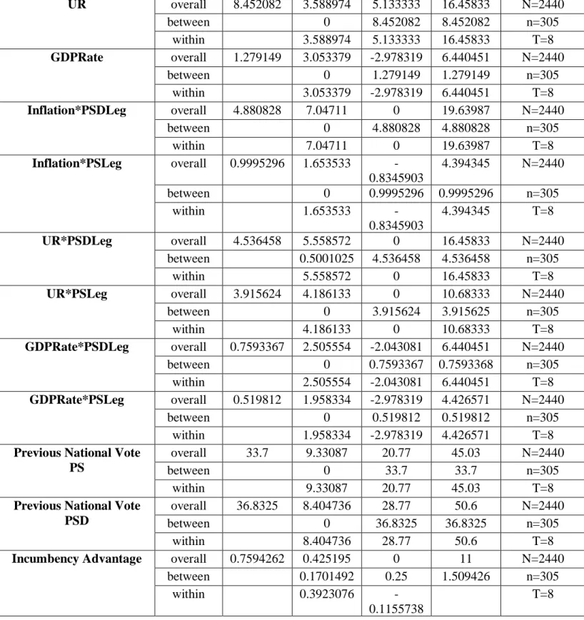
Table 1 – Descriptive Statistics
Variable Mean Std. Dev. Min Max Observations
Local Vote Variation PSD overall -0.4032384
10.49275 -41.67766 62.28 N=1900
between 2.778255 -11.4475 7.64 n=305
within 10.16428 -42.13123 61.6171
T-bar=6.22951
Local Vote Variation PS overall 0.993416 10.65764 -39.87355 45.32 N=2330
between 2.435665 -11.44 7.524526 n=305
within 10.39812 -37.58149 42.9018
T-bar=7.63934
Local Lag PS overall 36.23219 14.88941 1.4 76.8 N=2378
between 10.74941 6.89 67.10125 n=305
within 10.34711 -5.511559 74.29969
T-bar=7.79672
Local Lag PSD overall 39.21491 16.74441 0.96 88.84 N=2083
between 14.48908 2.8275 72.4425 n=305 within 8.890185 -6.41759 79.91491 T-bar=6.82951 PSLeg overall 0.5 0.5001025 0 1 N=2440 between 0 0.5 0.5 n=305 within 0.5001025 0 1 T=8 PSDLeg overall 0.5 0.5001025 0 1 N=2440 between 0 0.5 0.5 n=305 within 0.5001025 0 1 T=8 Inflation overall 5.880358 6.529538 -0.8345902 19.63987 N=2440 between 0 5.880358 5.880358 n=305 within 6.529538 -0.8345902 19.63987 T=8
UR overall 8.452082 3.588974 5.133333 16.45833 N=2440 between 0 8.452082 8.452082 n=305 within 3.588974 5.133333 16.45833 T=8 GDPRate overall 1.279149 3.053379 -2.978319 6.440451 N=2440 between 0 1.279149 1.279149 n=305 within 3.053379 -2.978319 6.440451 T=8 Inflation*PSDLeg overall 4.880828 7.04711 0 19.63987 N=2440 between 0 4.880828 4.880828 n=305 within 7.04711 0 19.63987 T=8 Inflation*PSLeg overall 0.9995296 1.653533 -0.8345903 4.394345 N=2440 between 0 0.9995296 0.9995296 n=305 within 1.653533 -0.8345903 4.394345 T=8 UR*PSDLeg overall 4.536458 5.558572 0 16.45833 N=2440 between 0.5001025 4.536458 4.536458 n=305 within 5.558572 0 16.45833 T=8 UR*PSLeg overall 3.915624 4.186133 0 10.68333 N=2440 between 0 3.915624 3.915625 n=305 within 4.186133 0 10.68333 T=8 GDPRate*PSDLeg overall 0.7593367 2.505554 -2.043081 6.440451 N=2440 between 0 0.7593367 0.7593368 n=305 within 2.505554 -2.043081 6.440451 T=8 GDPRate*PSLeg overall 0.519812 1.958334 -2.978319 4.426571 N=2440 between 0 0.519812 0.519812 n=305 within 1.958334 -2.978319 4.426571 T=8
Previous National Vote PS
overall 33.7 9.33087 20.77 45.03 N=2440
between 0 33.7 33.7 n=305
within 9.33087 20.77 45.03 T=8
Previous National Vote PSD
overall 36.8325 8.404736 28.77 50.6 N=2440
between 0 36.8325 36.8325 n=305
within 8.404736 28.77 50.6 T=8
Incumbency Advantage overall 0.7594262 0.425195 0 11 N=2440
between 0.1701492 0.25 1.509426 n=305
within 0.3923076
-0.1155738
T=8