R E S E A R C H A R T I C L E
Open Access
Optimization strategies for metabolic networks
Alexandre Domingues
1,3, Susana Vinga
1,2, João M Lemos
1,3*Abstract
Background: The increasing availability of models and data for metabolic networks poses new challenges in what concerns optimization for biological systems. Due to the high level of complexity and uncertainty associated to these networks the suggested models often lack detail and liability, required to determine the proper optimization strategies. A possible approach to overcome this limitation is the combination of both kinetic and stoichiometric models. In this paper three control optimization methods, with different levels of complexity and assuming various degrees of process information, are presented and their results compared using a prototype network.
Results: The results obtained show that Bi-Level optimization lead to a good approximation of the optimum attainable with the full information on the original network. Furthermore, using Pontryagin’s Maximum Principle it is shown that the optimal control for the network in question, can only assume values on the extremes of the interval of its possible values.
Conclusions: It is shown that, for a class of networks in which the product that favors cell growth competes with the desired product yield, the optimal control that explores this trade-off assumes only extreme values. The proposed Bi-Level optimization led to a good approximation of the original network, allowing to overcome the limitation on the available information, often present in metabolic network models. Although the prototype network considered, it is stressed that the results obtained concern methods, and provide guidelines that are valid in a wider context.
Background
Current metabolic engineering processes allow to manipulate metabolic networks to improve the desired characteristics of biochemical systems [1]. These manip-ulations may lead to the maximization of the normal product yield or redirect the production to a flux that was residual or non-significant in the original network. The high level of uncertainty in metabolic network models knowledge makes it extremely difficult to deter-mine what are the required manipulations needed to attain a given objective. Since an heuristic approach to such problems does not allow to explore the maximum potential of metabolic engineering, two approaches are usually considered when modeling metabolic networks. Kinetic models describe the complete dynamics of the network, and have proven useful to implement
optimi-zation and control over the network, such as in [2]. The creation of reliable kinetic models involves the estima-tion of parameters, the complexity of this task increasing with the size of the network considered.
The second approach models the networks on the basis of reaction stoichiometry. Although easier to obtain, these models lack the ability to directly predict the dynamics of the system.
Several techniques have been proposed to optimize and infer network characteristics from these models. In [3] a platform that combines many of these methods is presented. Flux Balance Analysis (FBA) allows the deter-mination of the optimal flux distribution on a network described in terms of the stoichiometry of the reactions and yields reliable results in the study of metabolic sys-tems [4-6]. A review of the method can be seen in [7].
When optimizing a metabolic network for a given objective two distinct problems must be addressed. The first is to find which branch or branches must be
* Correspondence: [email protected]
1INESC-ID - R. Alves Redol 9, 1000-029 Lisboa, Portugal
Full list of author information is available at the end of the article
© 2010 Domingues et al; licensee BioMed Central Ltd. This is an Open Access article distributed under the terms of the Creative Commons Attribution License (http://creativecommons.org/licenses/by/2.0), which permits unrestricted use, distribution, and reproduction in any medium, provided the original work is properly cited.
manipulated. The second is to determine what type of alterations must be done. Strategies such as OptKnock [8] and the work in [9] address the first problem. In this work a strategy for the second problem is described.
The simulation and engineering of metabolic network models typically involves complex optimization proce-dures. Geometric Programming (GP), one of the techni-ques used in this paper, is a powerful mathematical optimization tool that can be applied to problems where the objective and constraint functions have a special form [10]. GP is of particular interest because it can solve large scale problems with extreme efficiency and reliability [11]. Furthermore it has been shown that a problem formulated in S-Systems form can be solved with GP after a minimum adaptation [12].
A common optimization problem is the maximization of the final concentration of a metabolite whose forma-tion competes with the natural objective of the cell (e.g. maximization of biomass). In this work, a prototype net-work with such behavior is taken as example and the corresponding optimization problem is solved with three alternative methods.
It is stressed that the emphasis of this work is on the methods and not the specific network considered. The key point of the paper consists in establishing properties of a number of optimization methods that may serve as guidelines when considering more complex networks.
This will be further explained in the next section. Results and Discussion
An overall view of the problem considered and paper contributions is first presented. Details may then be seen in subsequent sections.
The problem to consider consists in finding a control function, defined over a finite interval of operation time, such that the final concentration of a desired product is maximum. This product is yielded by a metabolic net-work that, depending on the control function, either produces it or a product that favors cell growth. In order to settle ideas, assume that the control variable u is such that it is constrained to be in the interval [0, 1], with u = 0 corresponding to only production of cell growth product and no production of the desired pro-duct, and u = 1 corresponds to the inverse situation. Values of u in between 0 and 1 correspond to a mixed production in a way that depends on the network dynamics.
Since the optimization is with respect to a time func-tion, this is an in finite dimensional problem. However we prove in this paper, using Pontryagin’s Maximum Principle [13], that the optimal control only assumes values of 0 and 1. This is a priori assumed by other
authors [14] and receives now a solid justification. It is a result valid for similar metabolic network problems that aim at optimizing a final yield (e.g. a concentration at the end of the optimization time interval, such as in [15]) and such that the control enters linearly in the network equations.
The significance of this result consists in the fact that, instead of searching the optimal control among piece-wise continuous functions assuming values between 0 and 1, one only has to look functions assuming the extreme values of 0 and 1.
Furthermore, in the case study considered, it is shown that the optimum has only one switch between 0 and 1. Therefore the search for the optimum is reduced to find the switching instant, treg, that leads to the maximum
final yield. Considering the structure of the metabolic network, this is intuitive: the optimum is achieved by first applying all cell resources to population growth and, after treg, to redirect them to desired production. If
treg is too small, the desired production rate is higher
during more time, but the cell population to which it applies is small. If treg is too big, there are many cells to
produce, but they only act during a small time interval. Hence, there is an optimum value for treg.
As mentioned in the Background section, a major pro-blem is the high level of uncertainty in the knowledge about metabolic network dynamics. In this respect we consider different optimization algorithms that assume various degrees of information about the system to be optimized.
The first is direct optimization. This assumes com-plete knowledge about the system and is included to establish a benchmark with which other methods may be compared.
The other two methods are variants of a bi-level algo-rithm designed in order to accommodate missing infor-mation on the network kinetics. Both cases differ from the type of inner-optimization: Geometric Programming in one case and Linear Programming in the other. Both methods lead to good approximations of the optimal control, with a slight advantage of the one relying on Geometric Programming.
Prototype network model
The optimization strategies were tested on a proto-type network that is a modified version of a previously one suggested in [16]. The choice of this network was due to its widespread use as a test benchmark for several optimization algorithms. A graphical represen-tation of the network is shown in Figure 1 associated with the following set of ordinary differential equations:
dx dt k v dx dt v v u v u dx dt v u dx dt v u v dx 1 2 1 1 4 5 1 1 2 3 3 2 3 4 = − = − − − = − = − ( ) ( ) d dt =v4 (1)
Here the states xi, i = 1,..., 5 are metabolite
concen-trations at the network nodes, vi, i = 1,..., 4 are fluxes
associated to the metabolic network branches and k is a constant parameter that represents the uptake of x1. In
the equations, u represents a control function that allows to redirect the flux between the branches x2 ®
x3and x2® x4. Assuming that x3represents a precursor
of the cellular objective (such as growth) and x5 the
desired product, if u(t) is biased towards the branch of v2this yields the formation of x3but little or no
produc-tion of x5. If u(t) is biased towards the branch of v3the
production of x5 will be affected by the low
concentra-tion of x3 (since there is a forward feedback). Thus,
there is an optimal profile for u(t) to maximize the con-centration of x5at the final time tfinal.
In the framework of S-systems [16] the prototype net-work is described by:
dx dt k x dx dt x x x dx dt x u h g h h g 1 2 3 1 1 1 2 1 2 3 2 3 2 11 21 23 22 32 = − = − =
(
− ))
= − = dx dt x x u x dx dt x g g h g 4 5 4 3 2 4 4 5 454 43 42 44 (2)where bi are the rate constants, gij and hij are the
kinetic orders. Table 1 shows the list of parameters. All the simulations using the prototype network assume x(0) = [0.8 0 1 0 0].
Direct optimization
Direct optimization uses model (2) with the set of para-meters from Table 1.
On a first approach, all possible integer values of treg
in the interval treg= [1, 30] were used to compute the
final product concentration x5(tfinal) where tfinal = 30s.
Figure 2 plots the resulting function J(treg) = x5(tfinal).
It is clear from Figure 2 that there is an optimal value for the time of regulation that maximizes the yield of x5.
For the network considered, the optimal time of regula-tion is treg= 9s. If u(t) switches from 0 to 1 before treg
the formed biomass will not be enough to maximize x5
(tfinal). On the other hand, if u(t) switches from 0 to 1
after treg, there will be more biomass but there time will Figure 1 Prototype network. The circles correspond to
metabolites and the arrows to fluxes with the reaction rates indicated.
Table 1 Parameters used in the prototype network
Param. Value Param. Value
a2 8 h11 0.5 a3 4.0556 h22 1.4224 a4 1.8397 h23 0.6109 a5 4.0556 h44 0.5829 b1 1 g21 0.5 b2 5.1179 g32 0.4171 b4 4.0556 g42 2.8274 k 0.8 g43 1.4646 g54 0.5
Figure 2 Results of the simulation using Direct optimization. The final product concentration is shown as a function of Treg. For
the value of Tregcorresponding to the dotted line there is a
not be enough time to produce the maximum possible amount of x5.
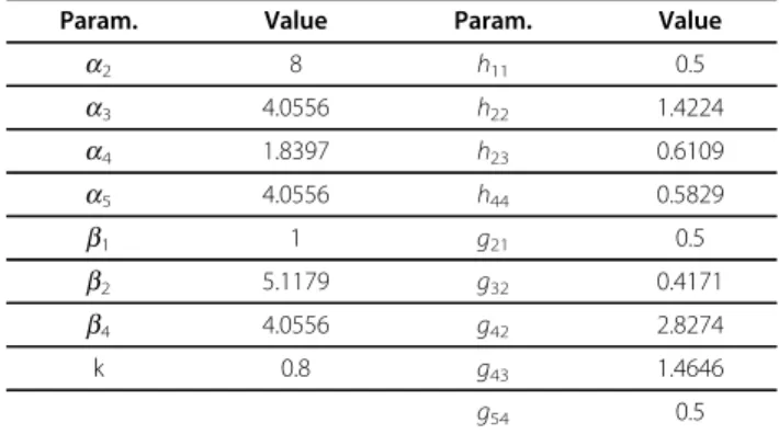
To illustrate better the behavior of the prototype net-work, simulations were made for treg = 4, treg= 9 and
treg= 14. The obtained optimal treg= 9 is compared in
Figure 3 with lower and upper values in order to show the different time evolution of the metabolites.
Bi-Level Optimization
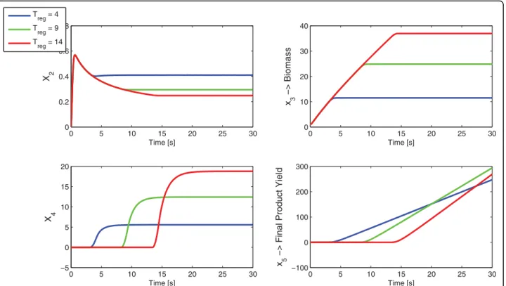
The Bi-Level optimization was used to test all the possi-ble values of treg. Figure 4 plots the normalized curves
for J(treg) = x5(tfinal) for the two optimizations,
inner-optimization using Geometric Programming (GP) and inner-optimization using Linear Programming (LP). By comparing Figure 4 with Figure 2 it can be seen that the profiles remain similar. The final product yield, x5
(tfinal), increases with treg until the optimal value is
reached, then it starts decreasing.
The optimal time of regulation obtained with both GP and LP on the inner optimization was treg = 9. As
shown mathematically in the methods section, the opti-mal control function is either 0 or 1, provided that the dynamics depends linearly on the control and the cost to optimize has only a final term.
In this case the dependency of the Hamiltonian function on u is linear (as given by (8) below). For the prototype considered,
(
( ) ( )
t ,x t)
=(
4 4 3xg43x2g42− 3 3 2xg32)
.Figure 5 shows a plot ofj(l(t), x(t)) obtained with a near-optimal control function u(t). As expected,j(l(t), x(t)) is negative for values smaller than treg, leading to an optimal
control u(t) = 0 and becomes positive for values larger than treg, leading to u(t) = 1. Thus, the optimal control is
obtained on the extremes of the allowed interval and furthermore, one single switch (from 0 to 1) is enough to achieve the optimal control. It should be remarked that, sincej(l(t), x(t)) is close to zero around t = treg, in
prac-tice, when using a numeric method there can be some jittering in the transition of the manipulated variable. Conclusions
For a class of networks in which the yield of the product that favors cell population growth (the “natural” pro-duct) competes with the desired product yield, with the manipulated variable affecting linearly the fluxes, it has been shown that the optimal control assumes only extreme values. While the implementation of this opti-mal control poses no challenge on in silico metabolic networks, on real metabolic networks complex bioengi-neering skills are required. Gene knockout manipula-tions do not adequate to this kind of control problem due to the long time scale associated with these techni-ques. The manipulation of specific enzyme levels,
con-trolled by modulating the expression of the
corresponding genes using promoter systems and
Figure 3 Comparison of three u(t) profiles. Three time profiles for the control function u(t) (above) and the corresponding product yield (below). The solid line is the optimal Tregobtained by Direct Optimization.
inducers, is a possible solution to this kind of control problem [14].
The use of a bi-level optimization strategy, that maxi-mizes the natural product in the inner level by manipu-lating the fluxes, leads to a good approximation to the optimal solution, with the advantage of not requiring the full knowledge of the network model. Real networks are extremely complex and exhibit relations between metabolites that are not always expected or fully under-stood. This gives emphasis to the need of good in silico models and also to the determination of the exact
branches to be modified when optimizing a network. Although the example network used is very simple, it has proved to be useful to test the optimization strate-gies but a more complex network should be used to confirm that the strategy can be scaled to a larger network.
Methods
The optimization problem
The optimization problem consists in relation to a non-linear state model of a metabolic network like (2), in selecting u(t) for tÎ [0, tfinal] such that:
J u
( )
=x5(
tfinal)
(3)is maximized under the constraint that u(t) Î [0, 1], ∇t ≥ 0.
The solution of the optimization problem is obtained using different approaches. Before accomplishing this task, Pontryagin’s Maximum Principle is invoked to establish a particular form of the optimal control func-tion for the class of problems at hand.
Optimization
The control function is now optimized in order to obtain a maximum yield of biomass at the end of the run-time (tfinal). Three different methods, assuming
var-ious levels of information about the network, are consid-ered in order to attain this goal.
The first method, direct optimization, is used as a benchmark to compare the results of the other methods.
Figure 4 Result of the optimization using the Inner Optimization with Geometric Programming (left) and Linear Programming (right). The profiles of the production of x5remain similar to the simulation using Direct optimization.
Figure 5 Plot ofj(l(t), x(t)) (9). This function changes sign at the optimal instant of control switching Treg.
The last two methods rely on a Bi-level optimization and illustrate a possible solution to the optimization problem when the information about the network is incomplete.
Direct optimization
The first method, Direct Optimization, is used mainly as a benchmark, to compare the results of the following methods. Since it is assumed that all the information about the network kinetics is known, the system of dif-ferential equations, described in (2) is used. Given a function that receives treg as input and outputs the final
yield of x5, this optimization tests all the possible values
of treg and returns the function J(treg) = x5(tfinal). The
value of treg that results on a maximum product yield is
then determined by solving a simple optimization problem.
The optimization was tested with two MATLAB func-tions: fmincon, from the standard optimization toolbox, that finds the minimum of a constrained nonlinear multi variable function, and simannealingSB from Sys-tems Biology Toolbox [17] that performs simulated annealing optimization.
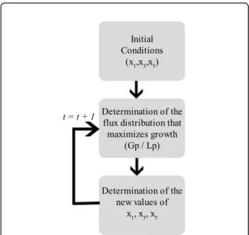
Bi-Level Optimization algorithm structure
The Bi-Level optimization algorithm was structured so as to accommodate missing information on the network kinetics. The boxed metabolites and fluxes from Figure 1 are a part of the network that might not be fully described in terms of kinetics. In this approach the missing kinetic information is replaced by stoichiometric data and flux balance analysis is used to obtain the proper flux distribution. Then, an inner optimization determines the fluxes during the batch time. The first step of the inner optimization process is to define the initial conditions of the input x1 and outputs x3, x5.
A valid distribution for the fluxes v1, v2, v3 and v4 is
then obtained.
After obtaining the flux distribution, new values for the input/outputs can be calculated by integrating their expressions in the considered time interval. During this time interval the function u(t) and the values of v1, v2,
v3 and v4 are kept constant. This process is repeated
along a time grid from t = 0 to t = tfinal. The time
inter-val for the integration was defined to be 1 second. The inner optimization process allows us to obtain the pro-duct yield, x5(tfinal), given a certain u(t), taking into
account a valid approximation of the network dynamics over the simulation time. The detailed fluxogram of the inner-optimization is shown in Figure 6.
The bi-level optimization algorithm can be repre-sented schematically as in Figure 7.
Inner-optimization using Geometric Programming
On the first implementation of the Bi-Level optimization algorithm the dynamics of the boxed metabolites from Figure 1 are used but, following the algorithm structure,
steady-state is assumed. Thus, x2 and
x
4 from (2)become: dx dt x x x dx dt x x u x g h h g g h 2 2 1 2 3 2 4 4 3 2 4 4 21 23 22 43 42 44 0 0 = − = = − = (4)
In this algorithm implementation, the inner optimiza-tion problem determines the profile of the metabolites, instead of fluxes, due to the nature of the equations. The metabolite concentrations are calculated at the beginning of each time interval, solving a Geometric Programming problem, and used with (2) to integrate the values of x1, x3and x5 during that interval.
Inner-optimization using Linear Programming
On the second implementation it is assumed that only stoichiometric information is available for the reactions
Figure 6 Inner-Optimization algorithm. Block diagram of the Inner-Optimization algorithm.
Figure 7 Bi-Level optimization formulation. Structure of the Bi-Level optimization.
inside the box of Figure 1. Assuming steady state, the equations of x2 and
x
4 become:dx dt v v u v u dx dt v u v 2 1 0 4 0 1 2 3 3 4 = − ×
(
−)
− × = = × − = (5)Figure 1 shows a regulation from x3 (Biomass) to flux
v3. Since stoichiometric models do not account for
feed-backs, the effect of x3 can not be integrated directly in
the equations. Assuming that the forward feedback leads to an over expression of flux v3, then a valid solution is
to model the forward feedback as a variation of the con-straints applied to flux v3. Setting flux v2 (precursor of
Biomass formation) as the objective function, the FBA problem is solved with the previous equations to obtain a valid and unique flux distribution at each time step. In the context of the inner-optimization, these fluxes are then used to calculate the values of the input/outputs. Pontryagin’s Maximum Principle
A general tool to solve dynamic optimization problems such as the one considered here is Pontryagin’s Maxi-mum Principle PMP [13].
Let x be the state of a dynamical system with control inputs u such that:
x F x u=
(
,)
, x( )
0 =x0, u t( )
∈U, t∈[
0,T]
(6)where F :ℜn×ℜ ® ℜn, U is the set of valid control inputs and T is the final time, assumed here to be constant.
The control function u must be chosen in order to maximize the functional J, defined by:
J u x Ti L x t u t dt
T
( )=( ( ))+
∫
( ( ), ( ))0
(7)
Whereψ is the cost associated with the terminal con-dition of the system and L the Lagrangian.
According to PMP, a necessary condition for the opti-mal control is that, along the optiopti-mal solution for the state x, co-state l and control u the Hamiltonian H is maximum with respect to u [13].
Comparing the cost (3) with the generalized case (7) and taking into consideration that, in the case at hand, given by (1), the dynamics vector field depends linearly on the control, it follows that
H( , , )λ x u = λ λ( , )x u (8)
where j(l, x) is a function that does not explicitly depend on u. Since, according to (8), the Hamiltonian is
linear in u, its maximum is obtained at the boundary of the admissible control set U.
Hence, this shows that, for the metabolic network (1), the control that optimizes (3) only assumes the values u = 0 or u = 1.
In the case at hand, we are interested in maximizing the final value of the state x5. Since the Lagrangian (L)
is zero, (7) becomes J(u) =ψ(xi(T)). Thus, the functional
J to be maximized is:
( ( ))x T =u T5( final) (9)
as shown before in (3).
Taking into account that, L = 0 the adjoint equations are reduced to
λ= − fxTλ (10)
The network is described by the system of ordinary differential equations in (2), if we consider the state model in the form of f(x, u), where u is the control function, calculating fx(x, u) is straightforward.
Thus λ λ 1 1 11 1 1 1 2 21 1 1 2 2 3 23 22 2 1 2 2 11 21 22 = = − − − − − h x g x x h h x h g h ( 3 32 2 1 3 4 343 42 2 2 2 23 3 1 4 3 32 42 22 1 g x u x ug x x h x g g g h − − − − = ) ( ) λ hh g g h g ux g x h x g x 23 43 44 54 1 2 4 2 43 3 1 4 4 44 4 1 4 5 54 4 4 42 − − − − − = λ −− = 1 5 5 0 λ (11)
The terminal conditions for the co-statesl are
λn T x x T
x
( )= ∂∂ |= ( )=([0 0 0 01]) (12) Since L = 0 the Hamiltonian is given bylTf(x). Substituting in the expression and after some manipu-lation, becomes: H t x t u t t k xh xg xh xh ( ( ), ( ), ( ), )λ λ λ = − − + −
(
)
(
1 1 1 2 2 1 2 3 2 22 11 21 23 ))
+ + − + − » » » » 5 5 4 54 3 3 232 4 4 444 4 4 343 242 3 3 23 ( ) ( x x x x x x g g h g g g22)u (13)that depends linearly on the control function u, as expected.
The derivative of the Hamiltonian in order to the con-trol function is:
H f x x x u T u g g g = = − + 3 3 232 4 4 343 242 (14)
This expression is the one that determines the number of switches between 0 and 1 of the control variable.
Acknowledgements
The work reported in this paper was performed within the project DynaMo -Dynamical modeling, control and optimization of metabolic networks, supported by FCT (Portugal) under contract PTDC/EEA-ACR/69530/2006. Author details
1
INESC-ID - R. Alves Redol 9, 1000-029 Lisboa, Portugal.2FCM-UNL - C Mártires Pátria 130, 1169-056 Lisboa, Portugal.3IST-UTL - Avenida Rovisco
Pais, 1000 Lisboa, Portugal. Authors’ contributions
AD helped in the research of the state of the art, implemented the software and drafted the manuscript. SV was involved in the creation and modeling of the prototype network, formulation of the optimization processes and helped to draft the manuscript. JML provided the mathematical basis for the optimization and control techniques and helped to draft the manuscript. All authors read and approved the final manuscript.
Received: 5 March 2010 Accepted: 13 August 2010 Published: 13 August 2010
References
1. Nielsen J: Metabolic engineering. Appl Microbiol Biotechnol 2001, 55(3):263-83.
2. Chu WB, Constantinides A: Modeling, optimization, and computer control of the cephalosporin C fermentation process. Biotechnol Bioeng 1988, 32(3):277-88, [Chu, W B Constantinides, A United States Biotechnology and bioengineering Biotechnol Bioeng. 1988 Jul 20;32(3):277-88.].
3. Rocha I, Maia P, Evangelista P, Vilaca P, Soares S, Pinto JP, Nielsen J, Patil KR, Ferreira EC, Rocha M: OptFlux: an open-source software platform for in silico metabolic engineering. BMC Syst Biol 4:45.
4. Edwards JS, Covert M, Palsson B: Metabolic modelling of microbes: the flux-balance approach. Environ Microbiol 2002, 4(3):133-40.
5. Varma A, Palsson BO: Stoichiometric flux balance models quantitatively predict growth and metabolic by-product secretion in wild-type Escherichia coli W3110. Appl Environ Microbiol 1994, 60(10):3724-31. 6. Schilling CH, Edwards JS, Letscher D, Palsson BO: Combining pathway
analysis with flux balance analysis for the comprehensive study of metabolic systems. Biotechnol Bioeng 2000, 71(4):286-306.
7. Llaneras F, Pico J: Stoichiometric modelling of cell metabolism. J Biosci Bioeng 2008, 105:1-11, [Llaneras, Francisco Pico, Jesus Research Support, NonU.S. Gov’t Review Japan Journal of bioscience and bioengineering J Biosci Bioeng. 2008 Jan;105(1):1-11.].
8. Burgard AP, Pharkya P, Maranas CD: Optknock: a bilevel programming framework for identifying gene knockout strategies for microbial strain optimization. Biotechnol Bioeng 2003, 84(6):647-57.
9. Rocha M, Maia P, Mendes R, Pinto JP, Ferreira EC, Nielsen J, Patil KR, Rocha I: Natural computation meta-heuristics for the in silico optimization of microbial strains. BMC Bioinformatics 2008, 9:499. 10. Koh K, Kim S, Mutapic A, Boyd S: GGPLAB: A simple Matlab toolbox for
Geometric Programming. 2006.
11. Boyd SP, Vandenberghe L: Convex Optimization. Cambridge University Press 2004.
12. Marin-Sanguino A, Voit EO, Gonzalez-Alcon C, Torres NV: Optimization of biotechnological systems through geometric programming. Theor Biol Med Model 2007, 4:38.
13. Lewis F, Syrmos V: Optimal Control John Wiley & Sons Inc. New York, 2 1995.
14. Kapil G, Gadkar RM III, F JD: Optimal genetic manipulations in batch bioreactor control. Automatica 2006, 42(10):1723-1733.
15. Gaspar P, Neves AR, Ramos A, Gasson MJ, Shearman CA, Santos H: Engineering Lactococcus lactis for Production of Mannitol: High Yields from Food-Grade Strains Deficient in Lactate Dehydrogenase and the Mannitol Transport System. Appl Environ Microbiol 70.
16. Sorribas A, Hernandez-Bermejo B, Vilaprinyo E, Alves R: Cooperativity and saturation in biochemical networks: a saturable formalism using Taylor series approximations. Biotechnol Bioeng 2007, 97(5):1259-77.
17. Schmidt H, Jirstrand M: Systems Biology Toolbox for MATLAB: a computational platform for research in systems biology. Bioinformatics 2006, 22(4):514-515.
doi:10.1186/1752-0509-4-113
Cite this article as: Domingues et al.: Optimization strategies for metabolic networks. BMC Systems Biology 2010 4:113.
Submit your next manuscript to BioMed Central and take full advantage of:
• Convenient online submission
• Thorough peer review
• No space constraints or color figure charges
• Immediate publication on acceptance
• Inclusion in PubMed, CAS, Scopus and Google Scholar
• Research which is freely available for redistribution
Submit your manuscript at www.biomedcentral.com/submit