Computational tools for data fusion and signal
processing of human gait
André Mendes Marques de Carvalho MSc in Bioengineering
Porto, 2013
André Mendes Marques de Carvalho
Computational tools for data fusion and signal
processing of human gait
Master thesis in Bioengineering
Supervisor: Prof. Dr. João Manuel R. S. Tavares Co-‐supervisor: Doutora Andreia Sousa
Faculdade de Engenharia da Universidade do Porto Porto, 2013
Acknowledgements
The work presented in this dissertation would not have been possible without the support and contribution of several people to whom I would like to address a special thanks:
• My supervisor, Professor João Tavares, for the availability, encouragement and support.
• To my co-‐supervisor, Andreia Sousa, for all the patience revealed during my visits, for all the opinions and shared resources.
• To my father for all the scientific support and help.
• To my family for being there whenever was needed and for encouraging me to follow my dreams.
• To all my friends who believed in me specially Rosa and Raquel.
Abstract
One of the most common motor actions is gait control. This is of critical importance and is highly affected by factors such as somatosensorial inputs, ground inclination and health problems. The goal of this study is to provide some computational tools for helping the analysis of electromyographic (EMG) and ground reaction force signals recorded during gait. The EMG signal will be analysed both in the time domain with classical techniques (wRMS / envelope) and also in the frequency domain, where patterns of muscle activation are expected to be found during cyclic movements. The ground force signals will be subjected to a classical analysis to provide the full centre-‐of-‐pressure (COP) and centre-‐of-‐mass (COM) kinematics as well as compute external power and work by both the independent and combined limb methods.
The main concern was to provide correctness in all equations and coding, secondly to provide new analysis tools and lastly to make the code as simple to use and modify as possible.
Some of the tools used (wavelet analysis) are computationally demanding so some optimization effort was done on the standard tools to provide one to two orders of magnitude improvement on these particular datasets.
Of course, having done the time-‐frequency analysis, the code also offers some trivial quality diagnostics on the EMG signal.
Finally, using the available dataset, some global analysis is presented. Hopefully these tools will be of any help to the health professionals.
Index
Acknowledgements ... iii
Abstract ... v
List of figures ... ix
List of Tables ... xii
Abbreviations ... xiii 1 – Introduction ... 1 1.1 – Overview ... 2 1.2 – Objectives ... 3 1.3 – Structure ... 3 1.4 – Main contributions ... 3
2 – Basis of human movement ... 6
2.1 – Introduction ... 6
2.2 – Gait ... 6
2.3 – Gait theories ... 7
2.4 – Typical GRF gait patterns ... 9
2.5 – Summary ... 10
3 – Instrumentation ... 12
3.1 – Introduction ... 12
3.2 – Force plate ... 12
3.3 – Electromyography ... 15
3.3.1 – Muscular system anatomy ... 16
3.3.2 – Motoneuron ... 18
3.3.3 – Action potential ... 19
3.3.4 – Neuromuscular junction ... 20
3.3.5 – Muscle contraction physiology ... 21
3.3.6 – Force production ... 21
3.3.7 – EMG electrodes ... 22
3.3.8 – Surface EMG signals ... 23
3.3.9 – EMG processing ... 25
3.4 – Time-‐frequency analysis ... 26
3.5 – Summary ... 29
4 – Development and implementation ... 32
4.1 – Introduction ... 32
4.2 – Main menu ... 32
4.3 – GRF data consistency ... 33
4.4 – GRF Filter choice ... 34
4.5 – Step interval calculation ... 40
4.6 – GRF processing ... 42
4.7 – General and test parameters ... 43
4.9 – Gait events ... 45
4.10 – Dynamics ... 46
4.11 – Plotting and numeric output ... 50
4.12 – EMG filter choice ... 51
4.13 – EMG algorithm implementation ... 52
4.14 – EMG wavelets and RMS calculation ... 54
4.15 – Calculating activation patterns ... 56
4.16 – Summary ... 62 5 – Results ... 64 5.1 – Introduction ... 64 5.2 – GRF results ... 64 5.3 – EMG results ... 68 5.4 – Summary ... 68
6 – Conclusions and future development ... 72
6.1 – Conclusions ... 72
6.1 – Future developments ... 72
References ... 73
List of figures
Figure 1 – walking cycle [adapted from (Perry 1992)] ... 7
Figure 2 – Two major walking theories (Kuo 2007) ... 8
Figure 3 – Typical GRF gait pattern ... 9
Figure 4 – Force platform and measured force components (Pais 2005) ... 13
Figure 5 – Force plate components (AMTI 2013) ... 13
Figure 6 – Force plate signal (vertical GRF) ... 14
Figure 7 – Channel saturation (excessive gain) ... 14
Figure 8 – Quantization noise (gain too small) ... 15
Figure 9 – Schematic of muscle components (MedicaLook 2013) ... 16
Figure 10 – Muscle fiber structure (Seeley, Stephens et al. 1995) ... 17
Figure 11 – Sarcomere representation (ProProfs 2013) ... 17
Figure 12 – Actin and myosin schematics (Kamisago, Sharma et al. 2000) ... 18
Figure 13 – Motor unit schematics (BaileyBio 2008) ... 19
Figure 14 – Membrane potential of a muscle cell (Wikipedia 2005) ... 19
Figure 15 – Synapse (Seeley, Stephens et al. 1995) ... 20
Figure 16 – Sarcomere changes during muscle contraction (Wikipedia 2007) ... 21
Figure 17 – EMG electrode examples [(Medizintechnik 2013) and (Bio-‐Medical Instruments 2013) ... 22
Figure 18 – Differential amplification of EMG signal ... 23
Figure 19 – Interference pattern (Quach 2007) ... 24
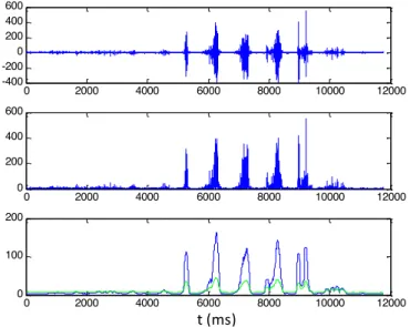
Figure 20 – Typical EMG signal ... 25
Figure 21 – EMG time processing example ... 25
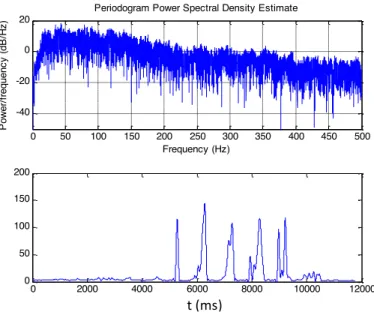
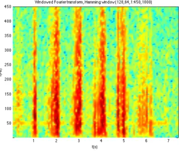
Figure 22 – EMG frequency domain processing example ... 26
Figure 23 – windowed Fourier transform time-‐frequency decomposition ... 27
Figure 24 – Choi Williams time-‐frequency decomposition ... 27
Figure 25 – Morlet wavelet time-‐frequency decomposition ... 28
Figure 26 – EMG signal ... 28
Figure 27 – Menu ... 33
Figure 28 – Trigger channel ... 33
Figure 29 – Trigger and suggested correction ... 34
Figure 30 – Second plate z-‐torque channel cross talking ... 34
Figure 31 – Raw vs filtered data ... 35
Figure 33 – Power density spectrum of lateral force signal ... 36
Figure 34 – Power density spectrum of forward force signal ... 37
Figure 35 – Power density spectrum of vertical force signal ... 37
Figure 36 – raw vs filtered data (8Hz) ... 38
Figure 37 – raw vs filtered data (70Hz) ... 38
Figure 38 – Step start and end calculation using 7% body weight as threshold ... 40
Figure 39 – Step start and end calculation using 1% body weight as threshold ... 41
Figure 40 – Algorithm schematics ... 43
Figure 41 – Input dialog ... 44
Figure 42 – Data file selection ... 45
Figure 43 – Gait events (vertical forces) ... 46
Figure 44 – COP and COM trajectory ... 47
Figure 45 – Instantaneous velocity of COM ... 48
Figure 46 – COM vertical displacement ... 49
Figure 47 – COM vs COP forward position ... 49
Figure 48 – Power during one cycle ... 50
Figure 49 – Numerical output ... 51
Figure 50 – PSD of raw and filtered EMG data ... 52
Figure 51 – EMG algorthm schematics ... 53
Figure 52 – EMG input dialog ... 53
Figure 53 – Gait intervals ... 54
Figure 54 – EMG analysis plot output ... 55
Figure 55 – EMG numeric output ... 56
Figure 56 – Combined plot of EMG wavelets analysis ... 57
Figure 57 – EMG wavelet analysis for slow sub-‐maximum contraction ... 58
Figure 58 – EMG wavelet analysis for slow maximum contraction ... 58
Figure 59 – EMG wavelet analysis for fast sub-‐maximum contraction ... 59
Figure 60 – EMG wavelet analysis for fast maximum contraction ... 59
Figure 61 – Combined plot of EMG wavelets analysis slow sub-‐maximum contraction ... 60
Figure 62 – Combined plot of EMG wavelets analysis slow maximum contraction ... 60
Figure 63 – Combined plot of EMG wavelets analysis fast sub-‐maximum contraction ... 61
Figure 64 – Combined plot of EMG wavelets analysis fast maximum contraction ... 61
Figure 66 – a) step analysis of a pathological gait b) multiple step analysis of a pathological gait
... 66
Figure 67 – numerical output ... 67
Figure 68 –EMG graphical output ... 68
List of Tables
Table 1 – Error induced by filter with cut-‐off frequency of 8Hz on one data set ... 39 Table 2 – Error induced by an incorrect choice of threshold ... 41
Abbreviations
COM – Center of mass COP – Center of pressure EMG – Electromyography GRF – Ground reaction forces RMS – Root mean square
wRMS – Windowed root mean square
1 – Introduction ... 2
1.1 – Overview ... 2 1.2 – Objectives ... 3 1.3 – Structure ... 3 1.4 – Main contributions ... 31 – Introduction
1.1 – OverviewGait analysis is frequently referred as having started with Aristotle’s works on biology (Aristotle n.d.).
Borelli is also frequently quoted in this context (Borelli 1680-‐1681) although the decisive component for biomechanics was published a little later (Newton 1687) and so was not present in Borelli’s works.
Nowadays, Gait Analysis is a standard subject of almost every course in Biomedicine, Biomechanics, Physiotherapy, Sport, etc. PubMed quotes 11569 papers on the subject since 1977, with 1054 published in 2012. Google Scholar provides around 687000 hits on books, papers and thesis worldwide, with 14700 just in 2013.
In fundamental research, the final goal is, often, to understand the mechanisms associated with gait control. However, today gait analysis has evolved to a clinical tool where it is used to aid in surgical planning on cerebral palsy cases (DeLuca, Davis et al. 1997; Cook, Schneider et al. 2003; Lofterod, Terjesen et al. 2007), assess the efficacy of surgical interventions, evaluate the rate of deterioration in progressive disorders or evaluate the impact of medication and orthopedic aids (Pollo 2007). Quantitatively, it is used to identify gait patterns, speed of walking, mechanical work made by the main muscular groups during the diverse phases, etc. (Sousa 2009).
In order to study these mechanisms a range of data collecting devices can be used: force plates for registering the force exerted on the ground, EMG for detecting the muscular activity, video cameras for visual tracking particular anatomical points, accelerometers/gyroscopes and LIDAR for body part kinematics and many other techniques.
The array of raw data is usually combined to obtain the kinematics and dynamics of a particular joint, the time evolution of the contact with the ground (centre of pressure) or the time evolution of the centre of mass. EMG aims at providing directly the muscular activity and both time techniques (windowed standard deviation) and frequency techniques (spectral content, filtering, etc) are usually employed for processing. Also some integration of the multiple data streams is also necessary (data fusion), at least synchronizing and overlapping records.
These aspects are to be detailed in the next few pages.
1.2 – Objectives
To produce a set of computational tools to aid medical and para-‐medical staff in accessing patients with gait-‐related disorders. These tools are to be written in a language easily accessible to health professionals and must address the main data sources: multiple ground reaction force sensors and multiple surface EMG sensors. Data quality should be checked whenever possible. All output should be made available onscreen and also on a (cumulative) file for offline processing.
1.3 – Structure
The present work is divided into five chapters. In the first one a general overview of the work is made and its objectives are defined. In chapter two it is explained how an action is performed and the particular case of gait. The two major human gait theories are also described. In the third chapter a description of the material is made. It is explained how the EMG and force plates works and the physical meaning of their signals. In chapter four we explain how the code was developed, the choices made, it’s assumptions and efforts made to reduce computation time. Finally the conclusions and future developments can be found in chapter five.
1.4 – Main contributions
There are three main (original) contributions for this thesis:
• The fusion of data from a double force plate setup allowed the computation of all kinematic quantities of both the COP and COM with high accuracy and without the need for any other sensors or data.
• The implementation of a wavelet based EMG signal processing strategy is original and unpublished (as far as we know) and may allow for the detection of activation phases regardless of any adaptive RMS voltage threshold.
• The optimization of a (specific) wavelet transform package allowed for reasonable processing times in commodity grade computers.
The first one – that can be extended to 3-‐step systems -‐ allows quantitative studies on gait stability and other health related issues like prosthetic, chirurgic, drug or physiotherapeutic influence on gait recovery.
The second one explores the interest in avoiding EMG intensity-‐based inferences as they depend on location, muscular dynamics and quality of skin-‐sensor interface. As there are almost no non-‐linear effects, frequency-‐based techniques are
proposed idea is implemented but needs validation studies has we had almost no time (and available data) to test it.
The third one is much less bioengineering but was a hurdle needed to be overcome to allow the implementation of the wavelet time-‐frequency decomposition idea. Even if proved good, extreme computation times would make that idea unusable to the common health professional or even researcher.
Several other minor contributions are scattered throughout the code. As no code has been reused from any source (except the profoundly optimized wavelet transform) and algorithmic choices and implementation details are not inspired on any paper, book or software, they are all original contributions, but are mostly trivial consequences of the current state of the art and so are not included here.
Chapter II – Basis of human movement
2.1 – Introduction 2.2 – Gait
2.3 – Gait theories
2.4 – Typical GRF gait patterns 2.5 – Summary
2 – Basis of human movement
2.1 – IntroductionThe complexity of the motor system is reflected on the complexity of the actions humans can achieve (Enoka 2008). These actions are a result of the interactions between the musculoskeletal and nervous systems, the first acting as a support and the second as the coordinator (Ghez and Krakauer 2000). Being so, all movement is achieved by the coordinated response of the muscles to neural commands (Bawa 2002).
Some of the most common motor action are the postural control and gait control. The postural control is a rather complex skill based on the interactions of dynamic sensory-‐motor processes and can be separated into two main functional goals: the postural orientation and postural equilibrium (Horak 2006). As for the Gait control this is a complex action in which the body COM is continuously unbalanced so the body weight is transferred from one leg to another with the minimum energy consumption (Alonso, Okaji et al. 2003).
For a motor action to take place it is needed a proper alignment of all body sections so it can maintain its stability despite all the unbalancing forces (Mackey and Robinovitch 2006). This way motor control can be defined as all the processes from which the nervous system, based on visual, vestibular and somato-‐sensory inputs, controls the musculoskeletal system to create coordinated movements and skilled actions while maintaining body posture (Júnior and Barela 2006).
The main goal of this chapter is to make a small explanation on how gait works, the main gait theories and what is a typical gait pattern.
2.2 – Gait
The primary goal of walking is the locomotion of the body from one place to another. To achieve this humans alternate their support from one leg to another, always keeping one foot on the ground, in an action where the body center of mass is displaced from its regular position allowing for the body to move forwards. The movements that take place during walking are cyclic and optimized to decrease energy expenditure (Silva 2009).
During regular walking a person needs to be able to maintain movement patterns, be able to maintain a dynamic equilibrium between the body center of mass and the moving support and to change his movement pattern in response to any external disturbance. The Walking cycle is every movement that occurs between the
initial contact of one foot in the ground and the instant that foot touches the ground again (Monteiro 2004).
Each walking cycle has two steps, one for each leg, and it is divided by two main actions, the support and the swing (Figure 1). The step refers to the contact between the foot and the ground and it correspond to 60% of the cycle time. The swing corresponds to the other 40% and is the time in which a leg is progressing thru space (Rose and Gamble 1998).
Figure 1 -‐ Walking cycle [adapted from (Perry 1992)]
As to the mechanical forces during gait there are two types: internal and external. The external forces are the gravity and ground reaction force (which can be measured with a force plate). Acting to oppose those forces are the internal forces. The internal forces corresponds to all the forces exerted or absorbed by muscles, ligaments, tendons and bones that work in order to counterbalance the external forces and support the body weight (Norkin and Levangie 1992).
During gait the COM describes a sinusoidal trajectory in the lateral and vertical displacements with 2 maxima in the vertical plane (two wave cycles) corresponding to the COM above COP for every step and one full wave cycle for the lateral displacement corresponding to the transition of the COP from one leg to another (Gard, Miff et al. 2004)
2.3 – Gait theories
The two prevailing models on human walking are the inverted pendulum and the six determinants of gait (Saunders, Inman et al. 1953), shown schematically in Figure 2. The six determinants of gait are the (proposed) set of 6 sub-‐actions of each step that seem to minimize the energetic cost of locomotion by reducing the vertical
and lateral displacement of the COM. They are the pelvic rotation, pelvic tilt, knee
flexion in stance phase, ankle flexion/extension mechanisms, knee mechanisms and lateral displacement of the pelvis. The last one reduces the lateral displacement of the
COM while the others reduce the vertical displacement. Unfortunately a closer look at the gait process showed that some of the determinants did not reduce the waving movements of the COM and also that a voluntary reduction of these movements increased the energy expenditure (Kuo and Donelan 2010). The coexisting inverted pendulum theory states that it is energetically benefic for the supporting leg to remain rigid creating an inverted pendulum, where the kinetic energy is converted into potential energy and vice versa. Unfortunately this model does not predict any energy expenditure at all during walking and is geometrically inconsistent during the double support phase.
Figure 2 -‐ Two major walking theories (Kuo 2007)
A little more realistic and less known theory is the passive dynamic walking
theory (McGeer 1990), that sophisticates the inverted pendulum theory by
incorporating the details of the heel-‐strike collision with ground. The author provided simulations and robotic samples proving the system is capable of passive stable locomotion on a small slope (downwards) and later others demonstrated that robots based on this model can move in flat ground with minimal energy expenditure (Collins, Ruina et al. 2005).
A model agnostic (phenomenological) approach divides the step into four phases: (i) ground strike, in which the foot touches the ground with much positive work from the quadriceps; (ii) the pre-‐load, in which the elastic energy is stored into the Achilles tendon and the quadriceps continue doing positive work; (iii) the propulsion, with major positive work done by the anterior tibialis; (iv) the swing, where no force is being exerted to the ground. In the swing phase, despite the absence of ground contact some muscular activity can still be found in anterior tibialis, hallucius and digitorum longus extensor (Norkin and Levangie 1992).
2.4 – Typical GRF gait patterns
The gait patterns can be influenced by almost any variable such as age, weight, diseases, strength, walking surface, etc. (Whittle 2007). Usually the gait patterns are obtained from force platforms that measure the ground reaction forces (GRF), equal and opposite to the ones made by the foot on the ground. Figure 3 is a representation of a typical healthy subject GRF pattern during half a walking cycle (between the pink bars). We can easily divide it in a (antero-‐posterior) breaking phase and an accelerating phase. For each leg, the point where no antero-‐posterior force is done (the location of the pink bars) is the point where the foot is under the hip (COP under the COM).
Figure 3 -‐ Typical GRF gait pattern
The vertical component of the GRF reaches up to around 120% of the subject body weight. It has two maxima more or less corresponding to the two extrema of the antero-‐posterior curve. The first half corresponds to the force exerted to stop the descending movement of the COM and the second one corresponds to the force exerted to push the COM up again (Perry 1992).
The lateral component is usually the least studied of the three but can be used to investigate foot instability (Winter 1990).
When the full set of forces is known, we can time integrate them and compute the impulse (velocity variation times mass) and with another integration compute the COM displacement with remarkable accuracy. On the premise that the human body is not statically stable and that a control system is necessary to stabilize the body, it is frequent to study the time evolution of the COP and COM. We’ll detail these a little later. 0 200 400 600 800 1000 1200 -100 0 100 lateral forces 0 200 400 600 800 1000 1200 -200 0 200 forward forces F( N ) 0 200 400 600 800 1000 1200 -1000 0 1000 vertical forces t (ms)
2.5 – Summary
Gait is a complex action that involves the precise coordination between the musculoskeletal and nervous systems, the first acting as a support and the second as the coordinator. This is a cyclic action optimized to minimize energy expenditure where the COM describes a sinusoidal trajectory in the lateral and vertical axis and whose support keeps alternating from one leg to the other.
There are two main gait theories, the inverted pendulum and the six determinants of gait. The first one are a set of 6 sub-‐actions of each step that seem to minimize the energetic cost of locomotion by reducing the vertical and lateral displacement of the COM and the second states that it is energetically benefic for the supporting leg to remain rigid creating an inverted pendulum, where the kinetic energy is converted into potential energy and vice versa.
The gait patterns can be influenced by almost any variable. These have very distinctive features and can be used to numerous studies. They can be obtained from force platforms that measure an equal and opposite force to the one made by the foot on the ground.
Chapter III – Instrumentation
3.1 – Introduction 3.2 – Force plate 3.3 – Electromyography
3.3.1 – Muscular system anatomy
3.3.2 – Motoneuron
3.3.3 – Action potential
3.3.4 – Neuromuscular junction
3.3.5 – Muscle contraction physiology
3.3.6 – Force production
3.3.7 – EMG electrodes
3.3.8 – Surface EMG signals
3.3.9 – EMG processing
3.4 – Time-‐frequency analysis 3.5 – Summary
3 – Instrumentation
3.1 – IntroductionBiomechanical instrumentations give us the ability to study gait and postural patterns as well as all the variables and diseases that can change a normal pattern increasing energy expenditure and increasing the probability of a fall. This is especially important for elderly people as this is one of the major causes of death and health related problems (Stevens, Corso et al. 2006). It also allows to quantify motor impairments and to keep tracking of diseases progressions. This kind of instrumentation is also used in rehabilitation to monitor improvements on stroke patients.
To study the gait and postural control mechanisms, a large array of instrumentation is available, including force plates, feet pressure sensors, EMG sensors, inertial sensors, video processing systems, EEG, radar, LIDAR, eye tracking systems and many other techniques. However the force plate is almost universal as it gives us simultaneously the COP location and (with some math) the COM time evolution, allowing for a quantifiable measure of body stability and control.
It is known that ageing, injuries, footwear and many others factors contribute to an abnormal postural and gait pattern. As the feet reaches the ground in different angles or as the center of mass displaces from its regular position the stability movements required to hold the body change. Consequently, force plates must be dissimulated not to induce changes in normal gait.
To have some idea of the mechanisms used for body control, it also frequent to use surface EMG sensors. These are non-‐intrusive and will give a (very) rough idea of individual muscular action, allowing for a more detailed study of the control aspects of locomotion.
In this chapter we will discuss the main equipment used to analyze gait such as EMG and force plates, as well as the physiological principles behind an EMG signal. A brief explanation on how the EMG signal processing is done using wavelets is also made.
3.2 – Force plate
There are several types of force plates depending on its transducers. The most popular are based on Hall effect probes, strain gauges and piezoelectric crystals. They are all thermally sensitive sensors.
The Hall effect sensor produces a voltage as a response to a magnetic field, usually from a nearby magnet. They must be driven by a stable current and a voltage must be measured with high impedance. They are rugged devices but are not very accurate, can’t be used near power cables, etc..
Strain gauges change electrical resistance according to mechanical elongation. They are measured usually with a bridge setup but the current changes the electrical resistance so a warm-‐up time is needed. They are fairly accurate but don’t age well (the bonding of the sensor to the supporting metal moves) and so need regular recalibration.
Piezoelectric is a charge sensor, sensitive to elongation. Piezoelectrics have a wide sensing range and frequency response as well a very good linearity and aging properties and so are used from ultra sensitive devices (microphones) to high load devices (sensors between the car and the wall in car crash tests). However they are expensive, sensitive to external vibration and demand electrometer amplifiers.
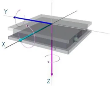
Figure 4 -‐ Force platform and measured force components (Pais 2005)
The most common force plates have six sensors to measure the three force components and the three torque components as shown in Figure 4 (each sensor is one-‐dimensional, so at least 6 are needed).
Figure 5 -‐ Force plate components (AMTI 2013)
Force plates usually have a non-‐serviceable embedded pre-‐amplifier system and also an external amplifier box, where the user can set the gain applied to each physical sensor (Figure 5) and switch on and off some filters (notch at line frequency,
low pass for anti-‐aliasing and force plate resonant frequency avoidance, etc). Of course the gain must be small enough as to not saturate the signal but as high as possible to minimize the quantization noise. The analog signal is then feed to an ADC and routed to a computer where a software tool manages the data acquisition and storage.
In order to transform the sensor information in force and torque
measurements a simple linear transformation is performed, including the information of the amplifier gains. An example of a correct final signal recording can be seen on Figure 6.
Figure 6 -‐ Force plate signal (vertical GRF)
Common problems can be seen in Figure 7 and Figure 8 and both preclude the usage of this data any further.
Figure 7 -‐ Channel saturation (excessive gain)
0 1000 2000 3000 4000 5000 6000 7000 8000 -100 0 100 200 300 400 500 600 700 800 points N 0 1000 2000 3000 4000 5000 6000 7000 0 100 200 300 400 500 600 points N t (ms) t (ms) F (N) F (N)
Figure 8 -‐ Quantization noise (small gain)
3.3 – Electromyography
EMG history can be traced back to Redi’s experiments (Redi and Platt 1686) on electric eel muscles. He found that electric eels have a highly specialized type of muscles that can produce electricity. One hundred years later (Fowler and Galvani 1793) a series of experiments were conducted that demonstrated that muscular contractions could be induced by the discharge of static electricity. Later (Du Bois-‐ Reymond 1848) the first evidence of electrical activity during voluntary contractions in human muscles were recorded using a galvanometer. In 1950 appeared the first commercially available electromyography system and subsequently the EMG field faced significant developments with the contributions of numerous researchers and the growing capabilities of the semiconductor industry (Ladegaard 2002)
The activation/deactivation of each muscle fiber generates an electrical field that can be measured -‐ the electromyographic signal (Basmajian and De Luca 1985). This way a direct measurement of the muscular activity can be made: the degree of muscular activation, the rate of force production, the number of motor units recruited, etc. However it is impossible to sense all muscle fibers in a muscle, much less in the body. So a few main muscles are selected and a single surface EMG probe is used in each one. Theoretically the surface EMG signal would correspond to the sum of all motor units action potentials (supra citæ). But each fiber signal crosses different tissues and impedances (changing in time) and other sources contaminate this as well, also dynamically. In order to better understand the quantities measured by the EMG first we need to understand how the muscle works.
4240 4250 4260 4270 4280 4290 4300 4310 4320 4330 4340 640 645 650 655 660 665 670 points N t (ms) F (N)
3.3.1 – Muscular system anatomy
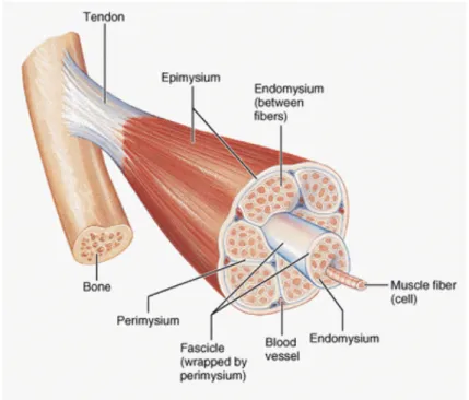
The human body has over 600 skeletal (voluntary) muscles. Each one is a hierarchical structure that contains fascicles, muscle fibers, myofibrils and actin and
myosin filaments as shown in Figure 9.
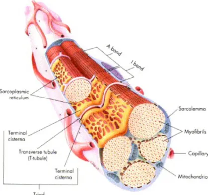
Each of these structures is surrounded by connective tissue as well as blood vessels and neurons (sensing). The connective tissue that holds the muscle together is called the epimysium, the one that covers the muscular fascicle is called the perymisium and muscular fibers are involved in the endomysium. Muscle fibers can be further decomposed into myofibrils, sarcoplasmatic reticulum and T-‐tubes as seen on Figure 10. These are of fundamental importance during muscular recruitment.
Figure 9 -‐ Schematic of muscle components (MedicaLook 2013)
Each of these structures is surrounded by connective tissue as well as blood vessels and neurons (sensing). The connective tissue that holds the muscle together is called the epimysium, the one that covers the muscular fascicle is called the perymisium and muscular fibers are involved in the endomysium. Muscle fibers can be further decomposed into myofibrils, sarcoplasmatic reticulum and T-‐tubes as seen on Figure 10. These are of fundamental importance during muscular recruitment.
Figure 10 -‐ Muscle fiber structure (Seeley, Stephens et al. 1995)
The myofibrils are formed by highly organized sub-‐units called the sarcomers that are placed continuously on top of each other. This is the unit that’s responsible for the contraction of the muscle. The sarcomere is made of various regions and 2 major types of bundles, actin and myosine filaments that alternate with each other (Figure 11).
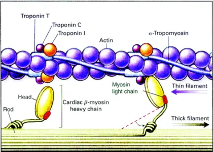
As shown in Figure 12 the actin filament is made of actin monomers, that have a specific binding site to the myosin molecules, and are fold in a double helix structure. They are also made of chains of an elongated molecule called tropomyosin that are placed above the actin binding sites and can cover up to seven actin molecules at once. The troponin is the last molecule of this complex and has 3 sub-‐units, one that binds to actin, other to tropomyosin and other to calcium ions.
The myosin filaments are made of numerous myosin molecules that have a golf club shape-‐like appearance. These molecules are made by two heavy-‐chain and four light-‐chains myosins.
Figure 12 -‐ Actin and myosin schematics (Kamisago, Sharma et al. 2000)
3.3.2 – Motoneuron
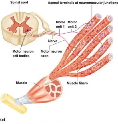
For a contraction to take place several structures of the nervous system must be involved. At the end of the central nervous system, in the spinal cord, specialized neurons (moto-‐neurons) connect with sets of muscle fibers and initiate the contraction (Kernell 2003). These sets of muscle fibers (Figure 13) are the minimum unit that can be recruited at any given moment and are called the motor unit.
Once a motor neuron is activated it generates a potential difference in its innervated muscle fibers resulting in an action potential (Figure 14). This happens every time an unbalanced distribution of ions inside and outside the cells is achieved (Loeb and Ghez 2000).
Figure 13 -‐ Motor unit schematics (BaileyBio 2008)
3.3.3 – Action potential
At rest, cell membranes are polarized (-‐70 to -‐90 mV) due to an excessive concentration of negative ions inside and positive ions outside the cell. This is a result of the good permeability of the membrane to the potassium ions and poor permeability to the negative charged ions.
Figure 14 -‐ Membrane potential of a muscle cell (Wikipedia 2005)
Once a cell gets sufficiently stimulated by the axon of the motor-‐neuron, an action potential occurs. This stimulus opens the sodium channels and the influx of sodium thru the membrane (osmotic pressure) will equalize potentials and even raise it up to +40 mV. This ion migration and potential change is a local effect that will affect the next sodium channels in the membrane, and then the next until the end of the fiber is reached. This is a propagating depolarization wave, from the enervation point to both ends of the fiber. Shortly after the opening of the channels they will close again and the potassium channels will finish expelling potassium from inside the cell, returning the membrane to its rest state(Seeley, Stephens et al. 1995).
3.3.4 – Neuromuscular junction
The neuromuscular junction is the region where the axon of the motoneuron connects to the muscle fiber creating a synapse (neuromuscular junction). The gap between the muscle fiber cell membrane (sarcolemma) and the axon terminal is called the synaptic cleft, Figure 15. Once an action potential reaches the axon terminal the calcium channels opens and calcium enters inside the axon cell membrane. This leads to the secretion of the content of several presynaptic vesicles within the synaptic cleft. The acetilcoline molecules bind to specific receptors on the within the postsynaptic membrane that allow sodium to get thru leading to an action potential in the muscle fiber.
Figure 15 -‐ Synapse (Seeley, Stephens et al. 1995)
3.3.5 – Muscle contraction physiology
Once the action potential reaches the synapse another one travels throughout the entire muscle fiber. Every time this reaches a T-‐tubule the calcium channels on the sarcoplasmic reticulum opens and the calcium stored in the sarcoplasmic reticulum enters the sarcoplasm. The calcium ions bind to the troponin that causes the tropomyosin to rotate exposing the actin binding sites. This leads to the binding of actin and myosin head that pull the actin filaments (Figure 12). This action is repeated during the contraction in every sarcomere within the muscle fiber until the H zone disappears, Figure 16.
Figure 16 -‐ Sarcomere changes during muscle contraction (Wikipedia 2007)
3.3.6 – Force production
If a motoneuron stimulus is strong enough to cause an action potential in its innervated fibers then all of them will contract as much as they can. This is called the all-‐or-‐none principle. During muscular contraction an increase in the force exerted by the muscle can be achieved in two ways. More muscle fibers can be recruited at any given time and/or each fiber (motor unit in fact) can be fired more often per unit of time. The first way of increasing force production is by increasing the strength of the
stimulus. This will increase the number of motor units recruited which in turn will increase the number of muscle fibers activated. The second way is related to the way the muscle fiber contracts. If a muscle fiber is stimulated a contraction occurs and shortly after it starts to relax. This means that the time averaged force exerted by that muscle fiber will be small. With the increase in the recruitment frequency so does increase the average force produced. Tetanus is the frequency above which the average force is maximum i.e. a new stimulus is sent even before the fiber is completely depolarized.
3.3.7 – EMG electrodes
The electric signals associated with muscular activity can be detected using EMG. There are two major types of electrodes, intramuscular and surface electrodes (Farina, Merletti et al. 2004) as shown in Figure 17. The intramuscular electrodes are used to study individual motor units. They are introduced with a needle and they get in direct contact with the muscles fibers. The main problems regarding intramuscular electrodes are the limited amount of muscle fibers that it can detect and the inconvenience related to invasive methods (Basmajian and De Luca 1985).
Figure 17 -‐ EMG electrode examples [(Medizintechnik 2013) and (Bio-‐Medical Instruments 2013)
As for the surface electrodes they are painless and have a larger area of detection. They deliver the sum of all the electric activity on the detection area, allowing the study of the global activity of a muscle. Its main disadvantages are its inability to recover the individual motor unit activity and its susceptibility to crosstalk, meaning that a vicinity muscle activity can be felt and promote misleading readings (Rau, Disselhorst-‐Klug et al. 1997). Almost universally EMG sensors are of differential configuration, strongly reducing the interference of power line induced noise.
3.3.8 – Surface EMG signals
As the EMG signal is of the order of tens of mV at the fiber, and one or two orders of magnitude less at the surface, amplification levels of 1000 to 10000 are common. To avoid interference, differential (or even multiple differential) systems are used, placing a pair of sensing elements along the fiber direction (pennation angle) one or two centimeters apart. Considering just one fiber, when the depolarization wave passes, it is seen twice with one of the lobes inverted Figure 18.
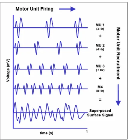
At the surface of the limb the signals from several motor units being recruited at different rates will arrive with varying delays and attenuations, producing the interference pattern that is recorded Figure 19
Figure 18 -‐ Differential amplification of EMG signal
The recruitment or firing rate for any given fiber (motor unit) is just of a few Hz but each wave is spectrally richer than that, say up to a few hundred Hz. The usage of high-‐pass filters to avoid motion artifacts eliminates the possibility of recovery of the firing rates and so of an important part of the relation of EMG and force.
The different distances from each fiber to the sensor introduce different delays to each wave so that simultaneous depolarization waves (maximum force) will not produce a maximum amplitude signal. But some particular combination of firing delays (sub maximal force) can produce a simultaneous arrival of the multiple waves and produce a maximum signal. Additionally, if there is movement the muscle fibers will move relatively to the skin and the surface sensors, increasing the complexity of the conduction, summing and EMG interpretation process. And all the other muscles in the neighborhood will also produce signals that can interfere with the ones we are trying to record. So, at best, the EMG signal recorded with single differential methods at the surface of the skin has only a qualitative relation with the force produced by some muscle. Also no two muscles or two experiences can be compared as the location and the adhesion of the sensors to the skin is not identical.
![Figure 1 -‐ Walking cycle [adapted from (Perry 1992)]](https://thumb-eu.123doks.com/thumbv2/123dok_br/15241706.1023034/23.892.261.688.314.549/figure-walking-cycle-adapted-perry.webp)