Meshless Difference Methods with Adaptation and High Resolution

Meshless Difference Methods with Adaptation

and High Resolution

Qun Lin

_{J.G. Rokne}

Abstract_{—Partial differential equations for domains}

with moving boundaries and moving interfaces are solved numerically using meshless finite difference schemes. The advantage of the approach is that it is easy to add nodes where there is a requirement of higher precision and delete nodes where the preci-sion requirements are less stringent. TVD and ENO schemes are considered in this context and some nu-merical examples are computed showing applications of the methods.

Keywords: meshless finite difference method, direc-tional difference quotient, points scattering and con-necting

1

Introduction

Moving interfaces and moving boundaries occur in many physical situations. Some examples are liquid-air inter-faces, ice melting in water, the deformation of bubbles, oil flowing under ice and the active interface during com-bustion in a solid fuel rocket engine.

The partial differential equations describing such prob-lems must take the interfaces and boundaries into account since material properties and behaviors are normally dis-continuous there. A version of the finite element methods is usually implemented in order to solve the problems nu-merically with the interfaces and boundaries handled in some fashion (see for example [6]). Other approaches in-clude the smoothed particle hydrodynamics used in the-oretical astrophysics computations (see [9, 8]) and radial basis function methods (see [3, 12]).

The finite element methods commonly used for these problems can be classified into methods

• where the grid is fixed and the interface is moving [16],

• where level sets are used [13, 11],

• where the grid deforms keeping pace with the moving discontinuities [15, 2, 14]

∗_{Department of Statistics, Xiamen University, Xiamen, China} †_{Department of Computer Science, The University of Calgary,}

Calgary, Alberta, Canada

• where the grid is refined locally to the discontinuities [4],

• where there is no grid (gridless methods) [17].

The commonality of the first four kinds of methods is a dependence on a grid, either fixed or deforming in some manner. More recently gridless methods have been inves-tigated. Examples of these are methods based on super-position of basis functions of various kinds and smoothed particle hydrodynamics. In this paper a meshless method based on finite differences is considered. In [10] a previous discussion of meshless finite difference methods was pre-sented and some examples were given. This paper can be viewed as a continuation of that paper to problems involving moving interfaces.

There is a clear advantage in using gridless methods for these problems in that a suitably chosen set of nodes can deform and move as the boundaries and interfaces change. This also means that more nodes can be added at critical points where there are large discontinuities thus improving the approximating properties of the solutions.

In this paper a meshless method is established where the only requirement is that a coordinate system is available. The effect of moving the nodes on the computational stencils is considered followed by refining and coarsen-ing of the stensils. A discussion of the construction of meshless difference methods with high resolution proper-ties and some examples concludes the paper.

2

Moving nodes

The problems considered here are two dimensional prob-lems whose solution are time-dependent velocity fields. These velocity fields are assumed to be computed at dis-crete time-steps. Because of this we call a velocity field at a particular time-step a time layer. A set of nodes

P = {P} on each time layer define the points where a given problem is approximated (and it should be noted that bynodeis meant both the name of the node as well as the coordinates of the node).

We first introduce some notations:

ν is the velocity field for the present layer,

(νx, νy) is the velocity at a point (x, y), β= ∆t·ν, whereβ is an increment and ∆t is a time step,

ξ=P+β, means that a new pointξis found by addingβ to node positionP .

In the following byν, β, ξ is meant the velocity compo-nent, increment and node position at a given pointx, y.

The advantage of meshless methods is that the position of a node can be changed adaptively according to the state of the solution as time progresses.

The progression of a solution from time layertk to tk+1

is now considered.

Two approaches are normally used:

(i): In the first approach the information from the solu-tion on the present layer is used for the following layer.

For this case a simplified directional difference quotient with respect to time is

u(ξ, tk+1)−u(P, tk)

∆t

= u(x+βx, y+βy, tk+ ∆t)−u(x, y, tk) ∆t

= ∂u ∂t +νx

∂u ∂x +νy

∂u

∂y +O(∆t) (1)

where

νx= βx ∆t, νy=

βy

∆t. (2)

In order to approximate νx∂u_∂x+νy∂u_∂y at a node P two known directional quotients ∆u

∆→l1

and ∆u

∆→l2

with respect

to space are considered. For this two nodes P1, P2 are

needed that are at distances ∆li = |P −Pi| from P, i= 1,2 as indicated in Figure 1.

The directional quotients can then be written as

∆u

∆

→

l1

=∆x1 ∆l1 ·

∂u ∂x +

∆y1

∆l1 ·

∂u

∂y +O(∆l1), (3)

∆u

∆

→

l2

=∆x2 ∆l2

·∂u ∂x +

∆y2

∆l2

· ∂u

∂y +O(∆l2). (4)

Setting ∆xi

∆li =Si,

∆yi

∆li =Ti, i= 1,2 we obtain

A ∆u ∆

→

l1

+B ∆u ∆

→

l2

= (AS1+BS2)∂u

∂x

+(AT1+BT2)∂u

∂y +O(∆l1+ ∆l2) (5)

whereA, B satisfy

AS1+BS2=νx, AT1+BT2=νy.

This solves to

A= νxT2−νyS2 S1T2−S2T1

, B= νyS1−νxT1 S1T2−S2T1

(6)

and we note that it is required that S1T2 = S2T1 and

P=Pi, i= 1,2.

Therefore we get from (1)

∂u ∂t =

u(ξ, tk+1)−u(P, tk)

∆t

−A ∆u ∆

→

l1

−B ∆u ∆

→

l2

+O(∆t+ ∆l1+ ∆l2) (7)

using (3), (4) and (5).

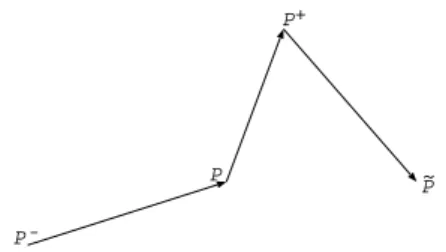
(ii): In this approach, indicated in Figure 2, the solution on the next layer is used as well. The computational cost is larger than in the first approach, but it can adapt more easily to the changes in fluids over time due to the forecasting of the future velocity field. The velocity field is extrapolated as follows:

ν(t+1

2∆t,·) = 3

2ν(t,·)− 1

2ν(t−∆t,·) (8) or

ν(t+1

2∆t,·) = 11

6 ν(t,·)− 7

6ν(t−∆t,·) + 1

3ν(t−2∆t,·) (9) and a β∗

is computed iteratively by means of dP_dt = ν(P, t)≈_∆β∗_t which leads to the recursion

βm+1= ∆t·ν(t+1

2∆t, P+ 1 2β

m_{), m= 0,1,· · · (10)}

whereβm_→β∗_{. Thus}

ξ=P+β∗

. (11)

Therefore the simplified directional quotient with respect to time is written as

u(ξ, tk+1)−u(P, tk)

∆t

= u(x+β

∗

x, y+β

∗

y, tk+ ∆t)−u(x, y, tk) ∆t

= ∂u ∂t +ν

∗

x ∂u ∂x +ν

∗

y ∂u

∂y +O(∆t). (12)

Similarly to the above, we can use the combination of two known directional quotients with respect to space to eliminate the influence of spatial directions from the movement of a node. That is, we have

A∗ ∆u

∆

→

l1

+B∗ ∆u

∆

→

l2

=ν∗

x ∂u ∂x+ν

∗

y ∂u

∂y+O(∆l1+ ∆l2) (13)

l l 1 β t t k = ξ P t t k = ₊₁ Δt 1 P 2 2 Δ Δ P

Figure 1: Directional difference quotients based on the present time layer

∗ β

t=t_k

ξ

+1

P

t=t_k

Δt 1 l₁ P 2 2 l Δ Δ P

Figure 2: Directional difference quotient using future layer

whereA∗

, B∗

satisfy

A∗_S

1+B∗S2=νx∗, A∗_T

1+B∗T2=νy∗

and we obtain

∂u ∂t =

u(ξ, tk+1)−u(P, tk)

∆t

−A∗ ∆u ∆

→

l1

−B∗ ∆u ∆

→

l2

+O(∆t+ ∆l1+ ∆l2) (14)

using (12) and (1).

In order to improve the approximation, we can construct a directional quotient on several time-layers as indicated in Figure 3.

For instance, to improve the approximation in the time direction, we have

u(P+β1, tk+1)−u(P−β−1, tk−1)

2∆t

=1 2

u(P+β1, tk+1)−u(P, tk)

∆t

+1 2

u(P, tk)−u(P−β−1, tk−1)

∆t =1 2 ∂u ∂t + 1 2ν 1 x ∂u ∂x+ 1 2ν 1 y ∂u ∂y + 1 4∆t

∂2_u

∂t2

+1 2ν

1

xβy1 ∂2_u

∂x∂y +· · ·+ 1 2 ∂u ∂t + 1 2ν −1 x ∂u ∂x+ 1 2ν −1 y ∂u ∂y −1

4∆t ∂2_u

∂t2 −

1 2ν −1 x β −1 y ∂2_u

∂x∂y − · · ·

=∂u ∂t +

1 2(ν

1

x+ν

−1

x ) ∂u ∂x+

1 2(ν

1

y+ν

−1

y ) ∂u

∂y +· · ·(15).

After eliminating the effect of moving a node we obtain second order precision in the time direction.

We can also combine time difference quotients to elimi-nate the effect of spatial shifts.

Au(P+β1, tk+1)−u(P, tk) ∆t

+Bu(P, tk)−u(P−β−1, tk−1) ∆t

+Cu(P−β−1, tk−1)−u(P−β∗, tk−2) ∆t

= 1

∆t[Au(P+β1, tk+1) + (B−A)u(P, tk)

+(C−B)u(P−β−1, tk−1) + (−C)u(P−β∗, tk−2)]

=A·∆t−1_{u(P, tk) +A}∂u

∂t +Aν

1

x ∂u ∂x

+Aνy1 ∂u

∂y +O(∆t) + (B−A)·∆t

−1_{u(P, tk)}

+(C−B)·∆t−1u(P, tk)−(C−B)∂u ∂t

−(C−B)ν−1

x ∂u

∂x−(C−B)ν

−1

y ∂u

∂y +O(∆t)

−(−C)·∆t−1_{u(P, tk)−2(−C)}∂u

∂t −(−C)ν

∗

x ∂u ∂x

−(−C)νy∗ ∂u

∂y +O(∆t) = ∂u

∂t +O(∆t) (16)

β

t t

k

= 1

β₋₁ P

t=t_k+1

t t

k

= ₋₁

Figure 3: Directional difference multi-layer construction

whereA, B, C satisfy

⎧ ⎨

⎩

A+B+C= 1, ν1

xA+νx−1B+ (νx∗−νx−1)C = 0, ν1

yA+ν

−1

y B+ (ν

∗

y −ν

−1

y )C = 0.

3

Node refining and coarsening

For each interior node, we have to construct a differ-ence scheme by means of arcs connecting adjacent nodes. Figure 4 shows two types of node stencils for star-like schemes of nine points.

If we need to increase the precision of the approximation then this can be done by combining directional quotients.

If a new node is inserted new arcs can be constructed to existing nodes. Usually, the quotient approximation of (1, 2, 3, 4) order needs a combination of (3, 6, 10, 15) nodes and (2, 5, 9, 14) directional quotients. Finding the combination coefficients requires the solution of a system of linear equations of the (2, 5, 9, 14) order. If any of the systems are singular then the singularity can be avoided by perturbating one or more of the nodes. An example of an order 2 approximation on 5 nodes requiring the solution of a 5×5 system of equations is given in [10], equations (12)-(14).

Except for the case of moving nodes, adaptive computa-tion can add and delete nodes according to the state of the local error. An error indicator for a computational region ΩL is therefore defined for eachtk as follows:

I(P, tk) =

u(P, tk)−uk(P)

, P ∈int ΩL, (17)

whereu(P, tk) is the current solution anduk(P) the ap-proximation such thatI(P, tk) reflects the approximating degree of the solution around the nodeP on a given time-layer. Here there are two computable constants C > 0 andRsuch that a local posteriori error estimation

u(P, tk)−uk(P)

≤C·R(uk(P)) (18)

holds.

Adding or eliminating nodes is carried through according to the following rule:

Let I∗

k = maxP∈ΩLI(P, tk), and let θref, θcoa be two

tolerances such that: 0< θcoa< θ_ref<1. Then

nodeP is added ifI(P, tk)> θ_ref·Ik∗ (19) nodeP is removed if I(P, tk)< θcoa·Ik∗. (20)

In order to balance the opposing requirements of ap-proximation degree and computational effort we add new nodes in ΩL if I is large and we remove current nodes from ΩL if I is small. In addition to this it is neces-sary to match the schemes for adding or removing nodes. When a new node is added, we must establish a differ-ence scheme based on this node. Similarly when a node is eliminated, we should at the same time delete the differ-ence scheme which is centered on this node. Sometimes, we need to also keep the balance between the number of entering arcs and that of exiting arcs for each node dur-ing addition or removal of nodes. As an example consider the scheme in Figure 5.

If we add a new node P0 with adjacent nodes

P1, P2, P3, P4, assuming thatP1, P2, P3, P4 are arranged

in anticlockwise order and that arc directions are

P4P1, P3P2, then these two arcs are removed and the

pathsP4 →P0 →P1, P3 →P0 →P2 are established. If

we remove the nodeP0with adjacent nodesP1, P2, P3, P4,

assuming that original paths areP2 → P0 →P4, P3 →

P0 →P1 then these two paths and the node P0 are

re-moved, and we replace them by the arcsP2P4, P3P1.

In order to simplify the programming we first mark all nodes which might possibly be used in the computation as well as the difference schemes on these nodes. At the same time we associate two flags to each node to indicate whether the scheme on that node will enter the compu-tational process at that moment. If that node is added at a given moment, then the corresponding scheme is

(a) (b)

P

0

P

1

P

3

P

4

P

6

P

7

P

0

P

1

P

2

P

3

P

4

P

5

P

6

P

7

P

8

P

8

P

2

P

5

Figure 4: Nine point star-like scheme

(a) adding a node

(b) removing a node

P

1

P

1

P

1

P

1

P

3

P

2

P

3

P

2

P

3

P

2

P

3

P

2

P

4

P

4

P

4

P

4

P

0

P

0

P

0

Figure 5: Adding and removing nodes

tivated and the computation is performed. If the node is removed, then the corresponding scheme is said to be dormant.

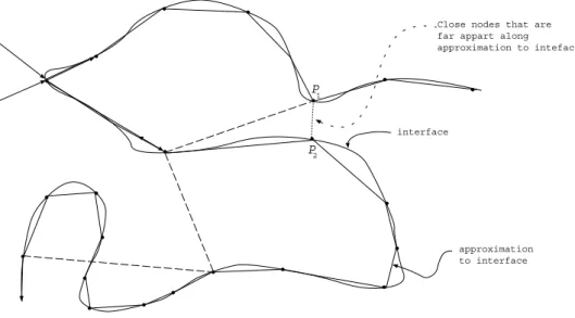
It must be pointed out that a weakness of Lagrangian methods is that the distance between two nodes may be changed significantly as a node moves. If there is a link between two nodes and they are moved so that they are far apart then the link can be removed if the nodes are in the interior of a region. If, however, the nodes are at the edge of a region, for example near a discontinuous in-terface, then we cannot modify the linking line between the nodes since we want to avoid destroying the inter-face which the scheme represents, see Figure 6. In this case, we should add new nodes on the linking line be-tween the two nodes along the approximating interface. If necessary, we should also consider interface indicators such as Level Sets. When we establish the corresponding schemes, it is still noted that the adjacent nodes must be established on one side of a moving interface so as to enhance the resolution for the interface.

In Figure 7 two examples of node progressions are indi-cated. In Figure 7(A) the nodes follow the flow of the fluids and the movements of the nodes are calculated as part of the process of approximating the equations result-ing in the node structure in the lower figure. The local a posteriori estimate (18) is used to estimate the accu-racy of the solution on that layer and, as shown in the figure nodes are added when condition (19)) requires it and deleted when condition (20) holds.

The sequence Figure 7(B) indicates that if there is an interface indicated by the dotted line then points on the interface should only be added not deleted even though condition (20) is satisfied.

4

Meshless TVD schemes

We now consider Total Variation Diminishing (TVD) schemes [7, 5].

The 2D scalar conservation law is stated as

ut+f(u)x+g(u)y= 0, (21)

or

ut+∇ ·F = 0, F = (f, g)T, ∇=

∂ ∂x,

∂ ∂y

(22)

and

∂f

∂u =a(u), ∂g

∂u =b(u) (23)

that is

ut+a(u)ux+b(u)uy= 0. (24) It is noted that, given any two independent directions l1, l2 we have

∂f ∂l1

= cosα1∂f

∂x+ cosβ1 ∂f

∂y, (25)

∂f ∂l2

= cosα2∂f

∂x+ cosβ2 ∂f

∂y (26)

where cosαi,cosβi are the directional cosines ofli, i = 1,2. Thus,

∂f ∂x =A

∂f ∂l1

+B∂f ∂l2

(27)

where

Acosα1+Bcosα2= 1,

Acosβ1+Bcosβ2= 0.

Similarly

∂g ∂y =C

∂g ∂l1

+D∂g ∂l2

(28)

where

Ccosα1+Dcosα2= 0,

Ccosβ1+Dcosβ2= 1.

Therefore, on a given node, we can construct a ”one-dimensional” scheme along a path passing through that node, and then establish a full scheme combining several different paths. Also, it will be shown in Section 7 that we can employ the splitting technique on different compu-tational paths. In this section, we consider the difference scheme

uk+1(P+) =uk(P)−r∗

( ˆf_Pk+_P−fˆ_{P P}k −) (29) wherer∗

= 2∆t/(|P+P|+|P P−

|) and

ˆ

fPk+_P ≡fˆ+(uk(P+), uk(P);r∗), (30)

ˆ

f_{P P}k − ≡fˆ−(u

k_{(P), u}k_(P−

);r∗

) (31)

are the numerical fluxes of this scheme, see Figure 8, which satisfies the following consistency condition

ˆ

f+(u, u;r∗) = ˆf−(u, u;r∗) =f(u). (32)

The scheme (29) will approximate the following equation

ut+A ∂f ∂l1

+B∂f ∂l2

= 0. (33)

From now on we do not consider moving the node. Doing this would just add a modification term written as

C1∗

∆f ∆l1

+C2∗

∆f ∆l2

to the spatial direction in the scheme.

Let L = max{l} where l is the length of an arc. We suppose that

|P+_P|

|P+_{P|+|P P}−_| →C ∗

, (L→0). (34)

P 1

P 2

interface

approximation to interface Close nodes that are far appart along approximation to inteface.

Figure 6: Close edge nodes

node added for the calculation for the time step step

node moved bassed on calculation in current time step

node removed in the current time step Initial

states

After one time-step

(A) (B)

Figure 7: Moving, adding and deleting nodes

P

P

P

+

-l

-l

+

Figure 8: Path through a node

For scheme (29), we have

(i): When conditions (32) and (34) hold, the scheme is consistent. This is because

ˆ

f+(u(P+), u(P);r∗) = ˆf+(u, u;r∗)

+( ˆf+)1(u, u;r

∗

)[u(P+_{)−u(P)] +O(L}2_{), (35)}

ˆ

f−(u(P+), u(P);r∗) = ˆf−(u, u;r∗)

+( ˆf−)₂(u, u;r∗)[u(P−)−u(P)] +O(L2). (36)

Thus

u(P, t+ ∆t)−u(P, t) ∆t

+fˆ+(u(P

+_{), u(P);r}∗_)−fˆ

−(u(P), u(P−);r∗)

(|P+_{P|+|P P}−_|)/2

=u

t+ ( ˆf+)1(u, u;r

∗

)u(P

+_)−u(P)

|P+_P|

· 2|P

+_P|

|P+_{P|+|P P}−_|

−( ˆf−)₂(u, u;r∗)

u(P−_)−u(P)

|P P−_|

· 2|P P

−

|

|P+_{P|+|P P}−_|+O(L)

=ut+ 2C

∗

·( ˆf+)1(u, u;r

∗

)∂u ∂l+

+2(1−C∗)·( ˆf−)₂(u, u;r∗)

∂u ∂l−

+O(L)

=ut+ 2C

∗∂fˆ+

∂l+

+ 2(1−C∗)∂fˆ− ∂l−

+O(L). (37)

(ii): If uk_{(P) → 0 as node P tends to infinity, then} scheme (29) implies that

allP

uk+1(P) = allP

uk(P), (38)

that is, scheme (29) is conserving and we note that (29) is the flux form. We also employ another two forms in

practice. Let

Qk_P+_P =

⎧ ⎪ ⎪ ⎪ ⎪ ⎪ ⎪ ⎨

⎪ ⎪ ⎪ ⎪ ⎪ ⎪ ⎩

⎧ ⎨

⎩

r∗f(uk(P)) +f(uk(P+))−2 ˆfPk+_P

uk(P+)−uk(P) , whenuk_(P+_)=uk_(P),

r∗

[( ˆf+)1(P) + ( ˆf+)2(P)],

whenuk_(P+_{) =u}k_(P).

(39) Here

ˆ fPk+_P =

1 2[f(u

k_{(P)) +f(u}k_(P+_))]

− 1

2r∗Q

k

P+_P ·[uk(P)−uk(P)] (40)

and scheme (29) can be written as

uk+1(P+) =uk(P)−1

2r

∗

[f(uk(P+))−f(uk(P−

))]

+1 2[Q

k

P+_P·(uk(P+)−uk(P)) (41)

+−Qk P P−·(u

k_(P)−uk_(P−

))]. (42)

This is called the viscosity form for scheme (29) and Qk_P+_P is called numerical coefficient of viscosity.

Moreover, scheme (29) can still be written as the follow-ing increment form

uk+1(P+) =uk(P)−CP Pk −·(u

k_(P)−uk_(P−

)) +D_Pk+_P·(u

k_(P+_)−uk_{(P)) (43)}

where

CP Pk − = 1 2(Q

k P P−+r

∗

akP P−), (44)

DPk+_P =

1 2(Q

k P+_P−r

∗

akP+_P) (45)

and

akP+_P =

⎧ ⎪ ⎪ ⎪ ⎪ ⎪ ⎪ ⎨

⎪ ⎪ ⎪ ⎪ ⎪ ⎪ ⎩

⎧ ⎨

⎩

f(uk(P+))−f(uk(P)) uk(P+)−uk(P) when uk_(P+_)=uk_{(P), ∂f}

∂u

k (P),

whenuk_(P+_{) =u}k_(P).

(46)

In the following several examples are given.

Example 1. Meshless explicit upwind scheme:

uk+1(P+)

=uk(P)−1

2r

∗

[f(uk(P+))−f(uk(P−

))] (47)

+1 2r

∗

|akP+_P| ·[uk(P+)−uk(P)]

−1

2r

∗

|akP P−| ·[u

k_(P)−uk_(P−

)]. (48)

The numerical flux of the scheme is

ˆ f_Pk+_P =

1 2[f(u

k_(P))−f(uk_(P+_))]

−1

2|a k P+_P| ·[u

k_(P+_)−uk_{(P)]. (49)}

From this it follows that the numerical coefficient of vis-cosity isQk

P+_P =r

∗

|ak P+_P|.

Here we note that the scheme becomes

uk+1(P+) =uk(P)−r∗[f(uk(P))−f(uk(P−))] (50)

whenak

P+_P ≥0 and it becomes

uk+1(P+) =uk(P)−r∗[f(uk(P+))−f(uk(P))] (51)

whenak

P+_P <0.

Example 2. Meshless Lax-Friedrichs scheme:

uk+1(P+) = 1 2[u

k_(P+_)−uk_(P−

)]

−1

2r

∗

[f(uk(P+))−f(uk(P−

))]. (52)

The numerical flux is

ˆ fk

P+_P =

1 2

f(uk_{(P)) +f(u}k_(P+₎₎

− 1

2r∗[u

k_(P+_)−uk_(P)].

(53) From this it follows that the numerical coefficient of vis-cosity isQk

P+_P = 1.

Example 3. Meshless Lax-Wendroff scheme:

uk+1(P+) =uk(P)−1

2r

∗

[f(uk(P+))−f(uk(P−))

+1 2r

∗2

(akP+_P)2·[uk(P+)−uk(P)]

−1

2r

∗2

(ak P P−)

2_·[uk_(P)−uk_(P−

)]. (54)

The numerical flux of this scheme is

ˆ fPk+_P =

1 2[f(u

k_{(P)) +f(u}k_(P+_))]

−1

2r

∗

(akP+_P)2·[uk(P+)−uk(P)]. (55)

From this it follows that the numerical coefficient of vis-cosity isQk

P+_P = (r

∗_ak P+_P)2.

In the following we will discuss so-called TVD property which is of special significance in the computation of sharply discontinuous interfaces.

The difference solution{uk_{(P)}, u}k_{(P)≡0 whenP is far} away from the computational region is given. We call

TV(uk) =L·

allP

|uk(P+)−uk(P)| (56)

the total variation of the difference solution. If the in-equality

TV(uk+1)≤TV(uk), ∀k (57)

holds, then the corresponding scheme is called a TVD scheme.

For a meshless TVD scheme, we will generalize the fol-lowing two familiar properties:

PROPERTY 1 (Harten lemma [7]) For the increment form (43) of scheme (29), if

CPk+_P ≥0, Dk_P+_P ≥0, C_Pk+_P +Dk_P+_P ≤1, ∀P (58)

then this scheme is a TVD scheme.

This is because

(a)uk+1(P+) =uk(P+)

−CPk+_P·[uk(P+)−uk(P)]

+Dk_{P P}˜ +·[u

k_{( ˜P)−u}k_(P+_{)], (59)}

(b)uk+1(P) =uk(P) +DkP+_P·[uk(P+)−uk(P)]

−Ck P P−[u

k_(P)−uk_(P−

)] (60)

(see also Figure 8). Subtracting equation (b) from equa-tion (a) we get

[uk+1(P+)−uk+1(P)]

= (1−CPk+_P−Dk_P+_P)·[uk(P+)−uk(P)]

+CP Pk −·[u

k_(P)−uk_(P−

)] +D_{P P}k˜ +·[u

k_{( ˜P)−u}k_(P+_{)]. (61)}

Taking the absolute values on both sides and summing for allP, we obtain

allP

|uk+1(P+)−uk+1(P)|

≤

allP

(1−C_Pk+_P−D

k

P+_P)· |u

k_(P+_)−uk_(P)|

+ allP

Ck P P−· |u

k_(P)−uk_(P−

)|

P

P

P P

+

-~

Figure 9: Harten lemma configuration

+ allP

DP Pk˜ +· |u

k_{( ˜P)−u}k_(P+_)|

= allP

{(1−C_Pk+_P −D

k P+_P)|u

k_(P+₎

−uk(P)|+C_Pk+_P|u

k_(P+_)−uk_(P)|

+Dk

P+_P· |uk(P+)−uk(P)|}

= allP

|uk_(P+_)−uk_{(P)|. (62)}

Hence TV(uk+1_)≤TV(uk_{) that is the scheme (42) is a} TVD scheme.

PROPERTY 2 For the viscosity form (42) of scheme (29), if

r∗

|ak_P+_P| ≤Qk_P+_P ≤1, (63)

then this scheme is a TVD scheme.

This is because the viscosity form (42) can be rewritten as

uk+1(P) =uk(P)−1

2(Q k P P−+r

∗

ak_{P P}−)

·[uk(P)−u(P−)]

+1 2(Q

k P+_P−r

∗

ak_P+_P)·[u

k_(P+_{)−u(P)] (64)}

From condition (63) and the Harten lemma it follows that

Qk_P+_P±r

∗

ak_P+_P ≥0, (65)

1 2(Q

k P+_P+r

∗

ak_P+_P)

+1 2(Q

k P+_P−r

∗

ak_P+_P)≤1 (66)

for allP, that is, this scheme is a TVD scheme.

Under the conditionr∗

|ak

P+_P| ≤1 and according to (63)

it follows that the meshless explicit upwind scheme is a TVD scheme since Qk

P+_P = r

∗

|ak

P+_P| ≤ 1. The

mesh-less Lax-Friedrichs scheme is also a TVD scheme since Qk

P+_P = 1. But the meshless Lax-Wendroff scheme is

not a TVD scheme since Qk

P+_P = (r

∗

ak

P+_P)2 does not

satisfy the condition (63). The above schemes usually are of order one because of the precision limitation of the node stencils.

5

Meshless ENO schemes

In order to improve the precision of TVD schemes, we must extend the node stencils using a meshless essential nonoscillatory (ENO) scheme. Previous work in this area can be found in [1, 3].

5.1

Successive extensions of a node stencil

LetP₁+_/2 be the middle point of the arc P+_{P and P}−

1/2

the middle point of the arc P P−_{, see Figure 10. The}

equation which we have to approximate is written as

∂u ∂t =A

∂f ∂l1

+B∂f ∂l2

(67)

wherel1=

−→

P P+_{, l} 2=

−→

P−

P.

First the construction of an integral averaging scheme is considered. The above equation will be integrated along

the path Γ =

−→

P−

1/2P +

1/2 and noting that |Γ|= 1 2(|

−→

l1 |+

|

−→

l2 |) we have

Γ

∂u ∂tds=−

Γ

A∂f ∂l1

+B∂f ∂l2

ds

=−A[f(u(P₁+_/2))−f(u(P))]

−B[f(u(P))−f(u(P−

1/2))]. (68)

Defining the path average ofu(x, t) as

uP = 1

|Γ|

Γ

u(s, t)ds (69)

we get

d

dtuP+A

f(u(P₁+_/2, t))−f(u(P, t))

|Γ|

+Bf(u(P), t)−f(u(P

−

1/2, t))

|Γ| = 0. (70)

In the following we will discuss the approximations of higher order tou(P₁+_/2) andu(P₁−_/2). In order to avoid dis-continuities when extending the stencils we employ direc-tional divided difference quotients to judge the smooth-ness degree ofuwithin the stencils.

P P

P

+

-P_1/2

-P_1/2+

Figure 10: Extending the node stencil

P

P

P +

- P1/2

-P+

1/2

Pk-1

P-k-1

2

P

1

P

-1

=

P P

0=

=

P

-2

Figure 11: Path throughP

Choose a path passing through P. The number of nodes in a local disc with center P is 2k − 1 :

{P−k+1, . . . , P−1, P0, P1, . . . , Pk−1 (see Figure 11). The

center ofPj−1Pk is denoted byPj/2. Let

u[P0] =uP0. (71)

The directional quotient of first order is

u[P0, P1] = u[P1]−u[P0]

|P1P0|

(72)

and the directional quotient of orderk−1 is

u[P0, . . . , Pk−1] = u[Pk

−1, . . . , P1]−u[Pk−2, . . . , P0]

|Pk−1P0|

(73) and we note the close connection with divided differ-ences in this development. The arc lengths |PjP0|(j =

2, . . . , k−1) can be calculated recursively from the arcs

|P1P0|,|P2P1|, . . . ,|PjPj−1|, that is

|P2P0|=

|P1P0|2+|P2P1|2−2|P1P0||P2P1| ·cosθ1,

|P3P0|=

|P2P0|2+|P3P2|2−2|P2P0||P3P2| ·cosθ2

· · ·

(see Figure 12).

A stencil will be adaptively extended by comparing the absolute values of the directional quotients. At first, the initial stencilS1 ={P0} is determined. To add a node,

we have two choices

S2= ⎧ ⎨

⎩

S1∪ {P−1},

or, S1∪ {P1}

(74)

that is, it will be decided whether to add a node to the left or to the right. We make our choice depending on the absolute values of directional quotients. If

|u[P0, P−1]≤ |u[P0, P1]|

then we add the node P−1, that is, S2 = S1∪ {P−1}.

Otherwise we add the nodeP1, that is,S2 =S1∪ {P1}.

The remainder follows by analogy. We prescribe that the nodes passing through fromP toPj have all been used if a nodePj is picked up on this path except forP. Thus, a stencil can finally be determined on the pathP−k+1→

· · · →P0 → · · · →Pk−1. Based on this stencil, we can

establish a Newton type interpolation formula with up to degreek−1 on the pathP₁−_/2→P →P₁+_/2:

u(Z) =u(P0) +

_u(Z)−u(P 0)

|ZP0|

· |ZP0|

=u(P0) +u[Z, P0]· |ZP0|

=u(P0)

+

u[P1, P0] +

u[Z, P0]−u[P1, P0]

|ZP1| · |ZP1|

· |ZP0|

=u(P0) +u[P1, P0]· |ZP0|

+u[Z, P1, P0]· |ZP1| · |ZP0|

=. . .

= k−1

j=0

u[Pj, . . . , P0]·Πj

−1

i=0|ZPi|

+u[Z, Pk−1, . . . , P0]·Πk_i=0−1|ZPi|

∆

= ΦP(Z) +O(Lk) (75)

where ∆= means that the quantity on the right is de-fined by the quantities on the left. Further we get the

P

2

P

0

P

1

P

3

P

4

θ1

θ3 θ2

Figure 12: Recursive calculation of difference quotient

approximating values on the both sides of the path as u−

P+ 1/2

= ΦP(P+

1/2) andu +

P−

1/2

= ΦP(P−

1/2) and we have

u−_P+ 1/2

= ΦP(P₁+_/2) =u(P₁+_/2, t) =O(Lk), (76)

u+_P−

1/2

= ΦP(P₁−_/2) =u(P₁−_/2, t) =O(Lk). (77)

Hence we obtain a semi-discrete scheme

duP dt +A

ˆ f(u−_P+

1/2

, u+_P+ 1/2

)−f(u(P, t))

|Γ|

+B

f(u(P, t))−fˆ(u−_P−

1/2

, u+_P−

1/2

)

|Γ| = 0 (78)

where ˆf(u−_{, u}+_{) is the numerical flux of ENO methods,}

which satisfy the following properties:

(i) (consistency) ˆf(u, u) =f(u)

(ii) (monotonicity) ˆf(↑,↓) which is not increasing for the first component and not decreasing for the second com-ponent

We can still construct the immediate difference-like scheme on each node.

The value of a node is noted asuP =u(P, t), and ˆfP+ 1/2

is the numerical flux. In order to construct ak’th order scheme, that is

A ˆ f_P+

1/2−f(u)

|Γ| +B

f(u)−fˆ_P−

1/2

|Γ|

=

A∂f ∂

→

l1

+B ∂f ∂

→

l2

P

+O(Lk) (79)

we require an interpolating function Ψ(Z) such that

1

|Γ|

P P+

AΨ(Z)dZ+ 1

|Γ|

P−_P

BΨ(Z)dZ

=f(u(P, t)) +O(Lk_{) (80)}

where Ψ(Z) satisfies the following integral averaging in-terpolation condition

1

|Γ|

P P+

AΨ(Z)dZ+ 1

|Γ|

P−_P

BΨ(Z)dZ=f(uP).

(81)

Taking ˆf_P+ 1/2

= Ψ(P+

1/2) we have

A ∂f ∂

→

l1

+B ∂f ∂

→

l2

P

=AΨ(P

+

1/2)−Ψ(P)

|Γ|

+BΨ(P)−Ψ(P

−

1/2)

|Γ| +O(L

k_{). (82)}

Hence we get a semi-discrete scheme

duP dt +A

Ψ(P₁+_/2)−Ψ(P)

|Γ| +B

Ψ(P)−Ψ(P₁−_/2)

|Γ| = 0. (83)

5.2

Linear combination ENO methods

The precision of the approximation in a smooth region can be increased by forming linear combinations of sten-cils. Suppose that there arek stencils

Sr(P) ={P−r, . . . , P0, . . . , Pk−1−r}, r= 0, . . . k−1

for a given difference.

From the above Newton interpolation, we can findk dis-tinct reconstructions u(r)

P+ 1/2

, r = 0, . . . , k−1 of u_P+ 1/2

on

each stencil. The LCENO (Linear Combination of ENO) scheme approximatesu(P₁+_/2, t) using linear combinations

of allu(r) P+ 1/2

:

u_P+ 1/2

= k−1

r=0

wru(_Pr+) 1/2

(84)

where it is required thatk−1

r=0wr= 1 in order to satisfy the consistency condition.

Moreover, ifuis smooth on all the stencils then we can finddr such that

k−1

r=0

dru(_Pr+) 1/2

=u(P₁+_/2, t) +O(L2k−1) (85)

and we still havek−1

r=0dr= 1 because of consistency.

In the smooth case, we require that wr = dr + O(Lk−1_{), r= 0, . . . , k−1 and we get}

k−1

r=0

wru(_Pr+) 1/2

−

k−1

r=0

dru(_Pr+) 1/2

= k−1

r=0

(wr−dr)(u(_Pr+) 1/2

−u(P₁+_/2, t))

k−1

r=0

O(Lk−1_)·O(Lk_{) =O(L}2k−1_{). (86)}

The method therefore has order 2k−1 precision, that is

u_P+ 1/2 =

k−1

r=0

wru(_Pr+) 1/2

=u(P₁+_/2, t) +O(L2k−1_{). (87)}

If there is a discontinuity in a LCENO scheme for a given stencil, then wr should be taken as zero. In practical computations,{wr}may be chosen as follows

wr= αr k−1

s=0αs

, r= 0, . . . k−1, αr= dr

(ǫ+βr)2 (88)

whereβr=O(Lk−1) andǫ >0 is introduced to avoid a vanishing denominator. Hence we have

wr=

dr

k−1 s=0ds

_ǫ+β

r

ǫ+βs

2

= dr

k−1 s=0ds

1−βs−βr

ǫ+βs

2 =

dr 1−O(βs−βs)

=dr+O(βs−βr)⇒βs−βr=O(Lk−1). (89)

6

Runge-Kutta like time discretization

In the above discussion, we obtained a semi-discrete schemeut=L(u), whereL(u) is an approximation for

−A∂f ∂l1

−B∂f ∂l2

.

In the following we will further consider the time dis-cretization so as to obtain a full-discrete scheme.

If the total variation norm is defined as ·=T V(·) then the Euler forward difference method

uk+1 =uk+ ∆t·L(uk) (90)

is TVD stable if the time step satisfiesδt≤∆t0 and we

have

(I+ ∆tL)(uk) ≤ uk. (91)

The general TVD Runge-Kutta time discretization scheme is

u(i)₌

i−1

s=0

(αisu(s)+ ∆t·βis·L(u(s))), i= 1, . . . , m,(92)

u(0) _=uk_{, u}(m)_=uk+1_{. (93)}

Assume that the coefficientsαis and βis satisfyαis ≥0, βis≥0,i

−1

s=0αis= 1. If the time step is chosen as

∆t≤c∆t0 andc= min

i,s αis

βis (94)

then the scheme is a TVD scheme.

There is no TVD Runge-Kutta scheme of fourth order such that αis ≥ 0, βis ≥ 0. Therefore the conjugate operator ˜LofLis defined in order to introduce the Euler backward difference method:

uk+1=uk−∆t·L˜(uk). (95)

For instance, for the equation

ut+A ∂f ∂l1

+B∂f ∂l2

= 0 (96)

we can define

L(u) =−f(u(P))−f(u(P

−₎₎

1

2(|P+P|+|P P

−_|) ,

˜

L(u) =−f(u(P

+_))−f(u(P)) 1

2(|P+P|+|P P

−_|) . (97)

Thus

1. The computations of quantities needed for Land ˜L are the same.

2. L is stable for the Euler forward difference.

3. ˜Lis stable for the Euler backward difference.

If αis ≥ 0, βis is negative and the operator ˜L is used instead ofL, then the scheme (99) is a TVD scheme under the following restriction of the time step

∆t≤c∆t0 andc= min

i,s αis

|βis|

. (98)

6.1

Linear multistep TVD schemes

The general linearmstep scheme is

uk+1= m−1

i=0

(αiuk−i+ ∆t·βi·L(uk−i)). (99)

Let the coefficientsαisandβissatisfyαi≥0,βi≥0 and m−1

i=0 αi= 1. If the time step is chosen as

∆t≤c∆t0and c= min

i αi βi

(100)

then the scheme is a TVD scheme.

There is still no TVD linear multistep scheme of fourth order such thatαi≥0 andβi ≥0. Therefore the conju-gate operator ˜Lis used.

If αi ≥ 0 and βi < 0 and the conjugate operator ˜L is used instead of operator L, then the scheme (98) is a TVD scheme under the following restriction of time step

∆t≤c∆t0 wherec= min

i αi

|βi|

. (101)

7

Splitting, compounding and coupling

break

The above only considers the construction of a scheme on a single path, for approximating the equation

ut+A ∂f ∂l1

+B∂f ∂l2

= 0. (102)

In order to obtain an approximation to the original equa-tion

ut+A ∂f ∂x +B

∂f

∂y = 0 (103)

we must employ a two path construction as shown in Figure 13. This results in

a A1 ∂f ∂ → l1

+B1

∂f ∂ → l2 +b A2 ∂f ∂ → l3

+B2

∂f ∂ → l4 +c

A3 ∂g

∂

→

l1

+B3 ∂g

∂ → l2 +d

A4 ∂g

∂

→

l3

+B4 ∂g

∂ → l4 =a A1

cosα1

∂f

∂x+ cosβ1 ∂f ∂y

+B1

cosα2∂f

∂x + cosβ2 ∂f ∂y +b A2

cosα3

∂f

∂x + cosβ3 ∂f ∂y

+B2

cosα4

∂f

∂x + cosβ4 ∂f ∂y +c A3

cosα1

∂g

∂x+ cosβ1 ∂g ∂y

+B3

cosα2

∂g

∂x+ cosβ2 ∂g ∂y +d A4

cosα3∂g

∂x + cosβ3 ∂g ∂y

+B4

cosα4∂g

∂x+ cosβ4 ∂g ∂y

= [(A1cosα1+B1cosα2)a

+ (A2cosα3+B2cosα4)b]

∂f ∂x +[(A1cosβ1+B1cosβ2)a

+ (A2cosβ3+B2cosβ4)b]

∂f ∂y +[(A3cosα1+B3cosα2)c

+ (A4cosα3+B4cosα4)d]

∂g ∂x

+[(A3cosβ1+B3cosβ2)c

+ (A4cosβ3+B4cosβ4)d]∂g

∂y. (104)

Solving the equations

(A1cosα1+B1cosα2)a+ (A2cosα3+B2cosα4)b= 1,

(A1cosβ1+B1cosβ2)a+ (A2cosβ3+B2cosβ4)b= 0,

(A3cosα1+B3cosα2)c+ (A4cosα3+B4cosα4)d= 0,

(A3cosβ1+B3cosβ2)c+ (A4cosβ3+B4cosβ4)d= 1

(105) we get

ut+a

A1 ∂f

∂

→

l1

+B1 ∂f

∂ → l2 +b

A2 ∂f

∂

→

l3

+B2 ∂f

∂ → l4 +c A3 ∂g ∂ → l1

+B3

∂g ∂ → l2 +a A4 ∂g ∂ → l3

+B4

∂g

∂

→

l4

=ut+ ∂f ∂x +

∂g

∂y = 0. (106)

Finally we will discuss the case of the system of convec-tion equaconvec-tions, that is, the system of 2D conservaconvec-tion laws

Ut+f(U)x+g(U)y = 0 (107)

where withu= (u1,· · ·, um)T

f(U) = ⎛

⎜ ⎝

f1(u1,· · ·, um)

.. .

fm(u1,· · ·, um) ⎞

⎟ ⎠,

g(U) = ⎛

⎜ ⎝

g1(u1,· · ·, um)

.. .

gm(u1,· · ·, um) ⎞

⎟

⎠. (108)

In the following we consider two approaches to such equa-tions.

(1): Splitting-coupling break

According to the above analysis, we have to solve the system of equations

Ut+A∗1

∂f(U)

∂

→

l1

+A∗2

∂f(U)

∂

→

l2

+A∗3

∂f(U)

∂

→

l3

+A∗

4

∂f(U)

∂

→

l4

+B∗

1

∂g(U)

∂

→

l1

+B∗

2

∂g(U)

∂

→

l2

+B∗

3

∂g(U)

∂

→

l3

+B∗

4

∂g(U)

∂

→

l4

= 0 (109)

atP.

We may employ a quarter time step ∆tto obtain

1 4Ut+A

∗

i+1

∂f(U)

∂

−→

li+1

+A∗

i+2

∂f(U)

∂

−→

li+2

= 0,

l2

l1

l3 l4

Figure 13: Combination of two paths

1 4Ut+B

∗

i+1

∂g(U)

∂

−→

li+1

+B∗i+2

∂g(U)

∂

−→

li+2

= 0,

(110)

i= 0,2. (111)

This can be solved using the method for scalar equations. Additionally, since

A∗

i+1

∂f(U)

∂

−→

li+1

+A∗

i+2

∂f(U)

∂

−→

li+2

=

A∗i+1

cosαi+1

∂f

∂x+ cosβi+1 ∂f ∂y

+A∗

i+2

cosαi+2

∂f

∂x + cosβi+2 ∂f ∂y

= (A∗

i+1cosαi+1+A∗i+2cosαi+2)

∂f ∂x

+(A∗i+1cosβi+1+A∗i+2cosβi+2)∂f

∂y

=A∗

i ∂f(U)

∂ −→ lA i (112) where A∗

i = (A

∗

i+1cosαi+1+A

∗

i+2cosαi+2)2

+(A∗

i+1cosβi+1+A∗i+2cosβi+2)2

and A∗ i = A∗ i, →

lAi = ((A

∗

i+1cosαi+1+A∗i+2cosαi+2)/A∗i, +(A∗

i+1cosβi+1+A∗i+2cosβi+2)/A∗i). (113)

and hence we can write (111) as

1 4Ut+A

∗

i ∂f(U)

∂

−→

lA i

= 0,

1 4Ut+B

∗

i ∂g(U)

∂

−→

lB i

= 0 (114)

or

1 4Ut+A

∗

i ∂f(U)

∂U · ∂U ∂ −→ lA i

= 0,

1 4Ut+B

∗

i ∂g(U)

∂U · ∂U ∂ −→ lB i

= 0 (115)

whereA∗

i ∂f(U)

∂U , B

∗

i ∂g(U)

∂U are computed by a local freez-ing approach. For instance, the value off

at P can be chosen as the arithmetic average of two points on the arc P−_P+ _{as A}∗

if

(1₂(U(P₁−_/2) +U(P₁+_/2))), or the Roe

averageA∗

if

(1₂(URoe(P₁−_/2) +U(P₁+_/2))).

In the following we consider a particular system of equa-tions. Let the matrixA∗

i ∂f(U)

∂U havemreal eigenvalues

λ1(U)≤λ2(U)≤ · · · ≤λm(U)

and a system of complete eigenvectors

r1(U), r2(U),· · ·, rm(U).

ThenA∗

i ∂f(U)

∂U can be diagonalized by a similarity trans-formation, that is,

R−1_(U)A∗

i ∂f(U)

∂U R(U) = Λ(U) (116)

where

Λ(U) = diag(λ1(U), . . . , λm(U)),

R(U) = (r1(U), . . . , rm(U)). (117)

SettingV =R−1_{U, we obtain}

1 8R

−1_U

t+R−1A∗ ∂f(U)

∂U R·R

−1∂U

∂

→

li = 0,

1 8Vt+ Λ

∂U

∂

→

lA i

= 0. (118)

Therefore the coupled equations can be broken into m independent equations ⎧ ⎪ ⎪ ⎪ ⎪ ⎪ ⎪ ⎪ ⎨ ⎪ ⎪ ⎪ ⎪ ⎪ ⎪ ⎪ ⎩ 1

8 (ν1)t+λ1 ∂ν1 ∂ → li

= 0,

.. .

1

which can also be solved using the method for scalar equa-tion. After gettingV we findU fromU =RV.

(2): Compounding-Roe like coupling break

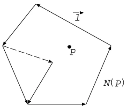
ForUt+f(U)x+g(U)y = 0, if both sides are integrated on the convex hullN(P) of the node stencil involving in the difference scheme atP we get

d dt

N(P)

U dΩ +

N(P)

(f(U)x+g(U)y)dΩ

= d dt

N(P)

U dΩ +

∂N(P)

(F ·n)ds= 0 (120)

where ∂N(P) is the boundary of N(P), n is the outer unit normal at a boundary line ofN(P) andF = (f, g). This is indicated in Figure 14.

The semi-discrete form for this is

A0

dU dt

N(P) =−

l∈N(P)

(F ·n)→

l ·∆l (121)

whereA0is the area ofN(P), which can be expressed as

the linear combination of nodal values onN(P). nlis the outer unit normal of boundary lineland ∆lis the length ofl.

The numerical flux can be written as

(F ·n)→ l =

1

2{(F·n)(U

−

→ l) + (

F·n)(U→+ l)

−

∂(F ·n) ∂U

→

l

·(U→+ l −U

−

→

l) (122)

where (U−

→ l

, U+ → l

) are theU values of at the sides of→l. As

in (32), the simple arithmetic average or Roe average of ∂(F·n)

∂U →

l is diagonalized by a similarity transformation:

R−1_(U) ∂(F ·n)

∂U

→

l

R(U) = Λ(U). (123)

Noting thatV→± l =R

−1_U±

→

l we have

(F ·n)→ l =

1

2{(F·n)(U

−

→ l

) + (F ·n)(U→+ l

)

−R(U)|Λ(U)|R−1_(U)(U+ → l

−U−

→ l

) (124)

= 1

2{(F ·n)(RV

−

→ l ) + (

F·n)(RV→+ l )

−(|λ1|r1,· · ·,|λm|rm)·(V→+ l −V

−

→

l ). (125)

Computational Example 1.Forward facing step prob-lem.

In Example 2, almost 8000 nodes are assigned for com-puting, and in Example 3, also 8000 nodes are assigned, and 2D shallow water equation is used.

This is a standard test example for high resolution meth-ods. The problem is as follows: In a windtunnel, 3 long and 1 wide a step is 0.2 high is located 0.6 from the left-hand end of the tunnel (see Figure 15).

We use an Euler system of equations of conservative type to describe the flow of fluids. Almost 12000 nodes are as-signed on one time-layer for computing, and a improved Wendroff scheme with a splitting flux and adaptive strat-egy was implemented as discussed in previous sections.

The initialization is a Mach 3 flow from the right. Re-flective bounds are set up along the walls of the tunnel, The in-flow and out-flow bounds are set up at the en-trance (right-hand end) and the exit (left-hand end). In the Figures 15-17 we present the result of the improved meshless splitting Wendroff like method of the computa-tion at timesta< tb< tc.

Computational Example 2. Double Mach reflection.

The computational domain for this problem is taken to be [0,4]×[0,1]. The reflecting wall lies on the bottom of the computational domain starting at 1/6 from the left-hand end (see also Figure 18). Approximately 8000 nodes are provided initially.

The initialization is a Mach 10 shock from the left posi-tioned on the bottom starting at 1/6 from the left-hand end and has a 600 _{angle with the axis. For the bottom}

bound, the post-shock condition is imposed for the part from left-hand end to 1/6 and a reflective condition is for the remaining distance. For the top bound of the com-putational domain, the flow values are set up to describe the motion of the Mach 10 shock. In Figures 18 and 19 several results of our meshless difference method are presented.

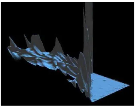
Computational Example 3. Problem of dam failure with the 2D shallow water equation.

A 200×200 computational domain is considered where there is dam which divides water storage into two equal parts. The upper part is 80 depth, and lower part is 20 deep. A segment on the dam body suddenly breaks. This segment is 75 long and 95 away from one side of the water storage. The flow of water obey 2D shallow water equation. Approximately 8000 nodes are provided initially.

In Figures 20 and 21 several results of our meshless dif-ference method are presented.

P

( )

P

l

N

Figure 14: Convex hull of node stencil atP

Figure 15: Forward facing step problem, a

Figure 16: Forward facing step problem, b

Figure 17: Forward facing step problem, c

Figure 18: Double Mach reflection, a

Figure 19: Double Mach reflection, b

Figure 20: Dam failure, a

Figure 21: Dam failure, b

References

[1] Abgrall, R., “On essentially non-oscillatory schemes on unstructured meshes: analysis and implementa-tion,” J. Computational Physics, V114, pp. 45-58, 1994.

[2] Azarenok, B. N., Ivanenko, S. A., Tang, T., “Adap-tive mesh redistribution method based on Godunov’s scheme,”Comm. Math. Sci.,V1, pp. 152-179, 2003.

[3] Cecil, T., Quian, J.. Osher, O., “Numerical meth-ods for high dimensional Hamilton-Jacobi equa-tions using radial basis funcequa-tions,”J. Computational Physics, V196, pp. 327-347, 2003.

[4] Devals, C. Heniche, M. Bertrand, F., Hayes, R. E., Tanguy, P. A., “A finite element strategy for the so-lution of interface tracking problems,”International Journal for Numerical Methods in Fluids, V49, pp. 1305-1327, 2005.

[5] Gottlieb, S., Shu. C. W., “Total variation diminish-ing Runge-Kutta schemes,” Mat. Comp., V67, pp. 73-85, 1998.

[6] Emmrich, E., Hyperbolische Erhaltungsgleichungen. Ph. D. thesis, Magdeburg, 1993.

[7] Harten, A., “High resolution schemes for hyper-bolic conservation laws,” Journal of Computational Physics, V49, pp. 357-393, 1983.

[8] Liu, G. R., Liu, M. B.,Smoothed Particle Hydrody-namics. A Meshfree Particle Method. World Scien-tific, Singapore, 2003.

[9] Monaghan, J. J., “Smoothed particle hydrodynam-ics,” Ann. Rev. Astron, Astrophys., V30, pp. 543-574, 1992.

[10] Lin, Q., Rokne, J., “Construction and analysis of meshless finite difference methods,” Computational Mechanics, V37, pp. 232-248, 2006.

[11] Ransau, S. R., Haegland, B., Holmen, J., “A fi-nite element implementation of the level set equa-tion,” Preprint Numerics, 4/2004, Norges Teknisk-Naturvitenskaplige Universitet. Downloaded from: http://www.math.ntnu.no/preprint

/numerics/2004/N4-2004.pdf, October 12, 2006.

[12] Sarra, S. A., “Adaptive radial basis function meth-ods for time dependent partial differential equa-tions,” Applied Numerical Mathematics, V54, pp. 79-94, 2005.

[13] Sethian, J. A.,Level Sets and Fast Marching Meth-ods.Cambridge University Press, 1999.

[14] Tang, T., “Moving mesh methods for computational fluid dynamics,” In: Recent Advances in Adap-tive Computation Eds.: Z. Shi, Z. Chen, T. Tang, and D. Yu, eds. Contemporary Mathematics, V383, American Mathematical Society, 2005, Proceedings of the International Conference on Recent Advances in Adaptive Computation, May 2004, Hangzhou, China, pp. 141-173, 2005.

[15] Tucker, P. G., “Transport equation based wall distance computations aimed at flows with time-dependent geometry,” NASA/TM-2003-212680, NASA Center for AeroSpace Information, Down-loaded from:

http://library-dspace.larc.nasa.gov/dspace/jsp/

bitstream/2002/13787/1/NASA-2003-tm212680.pdf, October 12, 2006.

[16] Udaykumar, H. S., Mittal, R. Rampunggoon, P., Khanna, Q.: “A Sharp interface cartesian grid method for simulating flows with complex moving boundaries,” J. Computational Physics, V174, pp. 345-380, 2001.

[17] Wu, N. J., Tsay, T. K., Young, D. L., “Meshless nu-merical simulation for fully nonlinear water waves,” International Journal for Numerical Methods in Flu-ids,V50, pp. 219-234, 2006.