An enriched meshless finite volume method for the modeling of material discontinuity problems in 2D elasticity

               

An enriched meshless finite volume method for the modeling

of material discontinuity problems in 2D elasticity

Abstract

A 2D formulation for incorporating material discontinuities into the mesh-less finite volume method is proposed. In the proposed formulation, the moving least squares approximation space is enriched by local continuous functions that contain discontinuity in the first derivative at the location of the material interfaces. The formulation utilizes space-filling Voronoi-shaped finite volumes in order to more intelligently model irregular geom-etries. Numerical experiments for elastostatic problems in heterogeneous media are presented. The results are compared with the corresponding so-lutions obtained using the standard meshless finite volume method and el-ement free Galerkin method in order to highlight the improvel-ements achieved by the proposed formulation. It is demonstrated that the enriched meshless finite volume method could alleviate the expecting oscillations in derivative fields around the material discontinuities. The results have re-vealed the potential of the proposed method in studying the mechanics of heterogeneous media with complex micro-structures.

Keywords

finite volume method, meshless method, material discontinuity, enrich-ment technique, Voronoi tessellation.

1 INTRODUCTION

The finite-volume method FVM is a numerical technique that provides approximate solutions to boundary value problems with partial differential equations. In this method, the computational domain is divided into smaller sub-domains, called as finite volumes, each containing one node point on the discretized geometry and the partial differential equation is satisfied in the integral sense over each finite volume. A distinctive feature of the method is the use of boundary integral instead of the domain integral, for satisfying partial differential equa-tion.

The mesh-based formulation of FVM is a well-established technique in a wide range of problems concerned with the mechanics of solids and structures, see Taylor et al. 2003, Fallah 2004, Cardiff et al. 2014, Escarpini Fil-ho and Marques 2016, Cavalcante and Pindera 2016 . However, for certain classes of problems, the heavy and rigid reliance of the mesh-based FVM on a mesh leads to some difficulties. Some of these difficulties are as follows

Liu 2009 :

• High computational cost and human-labor in creation of a quality mesh for domain with complex geometry,

• Additional computation as well as a degradation of accuracy in remeshing approach to deal with evolution problems, and

• Discontinuous nature in calculating stress fields, due to the element-wise continuous nature of the displacement field assumed in the mesh-based formulation.

These difficulties could be decreased by using a mesh independent formulation. For this purpose, meshless formulation of FVM, which is also named as MLPG5 by Atluri and Shen 2002 , has been introduced. This method has been accepted by many researchers and widely used for solving problems in solid and structural mechanics, see Batra et al. 2004, Han et al. 2005, Sladek et al. 2008, Hosseini et al. 2011, Soares et al. 2012, Ebrahimnejad et al. 2014, 2015, 2017 .

Interpolation of field variables by moving least squares approximation and integrating weak form of the equilibrium equation over local finite volumes in meshless FVM eliminates the need for mesh generation. Instead, it relies on background local finite volumes where each finite volume is independent of the others, i.e. they can be of any geometric shape and size and even using overlapped finite volumes are allowed. However, they should locate entirely inside the boundaries and their union should cover the whole domain. In addition, the high order of continuity inherits from moving least squares approximation, provides solutions with smooth derivatives

Abdullah Davoudi-Kia a N. Fallah a,b,*

a _{Department of Civil Engineering, University of}

Guilan, P.O. Box 3756, Rasht, Iran. E-mail: davoudikia@phd.guilan.ac.ir

b _{Faculty of Civil Engineering, Babol Noshirvani}

University of Technology, Babol, Iran. E-mail: fallah@nit.ac.ir

*Corresponding author

http://dx.doi.org/10.1590/1679-78254121

Received: June 14, 2017

throughout the domain. As a result, negligible pre-processing and post-processing costs of meshless FVM are the main attractive features over the prevalent mesh-based methods Atluri and Shen 2002 . Atluri and Shen 2002 have demonstrated that meshless FVM can be a simple and efficient alternative to the all-purpose FEM, due to its speed, accuracy and response stability.

In this paper the meshless FVM is applied to the material discontinuity problem which is an important issue in numerical modeling of heterogeneous media. It should be noted that heterogeneity is a ubiquitous property of solids and structures associated with features such as holes or inclusions that have an important role in the fail-ure Gdoutos 2005 .

The solution of problems in heterogeneous media typically involves discontinuity in gradient fields. In order to capture non-smooth property of the solutions, there are two essentially different techniques. The first tech-nique applies smooth polynomial approximation spaces and trusts in domain discretization that conforms to ma-terial discontinuities. The polynomial approximation spaces can be constructed by using either a mesh-based shape function or meshless approximation function. The alternative technique is based on ‘enrichment’ of smooth approximation space such that the domain discretization being independent of the material discontinuities. The enrichment will be accomplished by adding special weak discontinuous functions to the approximation space with unknown parameters that control the strength of the discontinuity.

The first above mentioned technique has been used by Cavalcante et al. 2007 within the mesh-based FVM framework for functionally graded materials and also by Li et al. 2003 in the 3D formulation of the MLPG meth-od to problems with singularities and material discontinuities. In the latter, the heterogeneous medium is sepa-rated into isolated, homogeneous parts and then continuity constraints are enforced at the interface to ‘reconnect’ the pieces. To accomplish the ‘separation’, meshless approximation function applied separately within each ho-mogeneous part and therefore domains of influence are truncated at the material interfaces. Also, local sub-domains, which partially cut by the interface, are redefined to locate entirely inside the boundaries. In spite of the simple concept of this technique, the presence of truncated domains of influence could introduce some mesh de-pendency into the solution Cordes and Moran 1996, Li et al. 2000 ; Furthermore, re- definition of local sub-domains and sub-domains of influence could be difficult and computationally expensive de Borst 2008 . The so-called enrichment technique has been applied both in the area of mesh-based and meshless methods. Melenk and Babuška 1996 enriched the standard finite element approximation, Belytschko and Black 1999 set up the frame of the extended FEM XFEM and Belytschko et al. 1996 implemented it within the EFG method for intro-ducing discontinuous derivatives into the solution. Batra et al. 2004 utilized this technique in the 1D meshless formulation of FVM to analyze heat conduction in a bimetallic circular disk. Recently, Yoon and Song 2014 and Hu et al. 2015 applied this technique in order to handle discontinuities in heterogeneous media. Using the en-richment technique is interesting since a fix and regular domain discretization can be applied and domain dis-cretization cost is reduced to a minimum An et al. 2011 . In this paper, based on the enrichment technique used already by Krongauz and Belytschko 1998 , a 2D formulation within the meshless FVM framework is proposed to handle material discontinuity.

The structure of the present paper is as follows. In the next section, the basic concepts including standard meshless FVM, moving least squares approximation and enrichment of approximation space are briefly described. A 2D formulation in modeling heterogeneous material within the meshless FVM framework is presented in sec-tion 3. Numerical examples and results to verify the capability of the formulasec-tion are presented in secsec-tion 4 and concluding remarks are given in the last section.

2 BASIC CONCEPTS

2.1 Standard meshless FVM

Most of the meshless methods, e.g. element free Galerkin EFG and smoothed particle hydrodynamics SPH , are based on global weak forms and required the use of background mesh in order to integrate the weak form of the equilibrium equation. On the other hand, the meshless local Petrov-Galerkin MLPG method satisfies the weak form over the local sub-domains. As a special case, MLPG5 Atluri and Shen 2002 chose the Heaviside step function as the test function. Consequently, domain integrals are vanished and integration is performed along the boundary of local domains. Satisfying local weak form denotes the momentum balance law over the local sub-domains that resemble the concept of FVM. Therefore, the MLPG5 method could be recognized as the meshless FVM Atluri et al. 2004 .

Let



be a domain bounded by



. Momentum balance principles for static problems are given by

, 0 ,

ij j bi for all x

where

σ

is the stress tensor and

b

is the body force measured per unit volume. The essential and natural boundary conditions are as follows

i

u

i u

u

=

on

G

_{, 2a}

i

t

i t

t

=

on

G

_{, 2b}

where

u

_and t are defined as the prescribed displacements and tractions, respectively.



_u is the global essential boundary and



t is the global natural boundary. Utilizing weighted residual method, weak form of the Equations

1 - 2 over I-th local finite volume



s enclosed by



s, can be written as

(

,

)

(

)

0,

s su

I I

ij j b v di ui u v di

s a

W + W - G - G =

ò

ò

3

where I

v is the test function for I-th local finite volume and



>>

1

is a penalty parameter which is applied to

impose the essential boundary conditions. In meshless formulations, a local approximation scheme will be applied to approximate the trial function; therefore, the essential boundary conditions cannot be imposed directly, a priori, but superimposed in a weak form. In this paper, the penalty method is applied to superimpose the essential boundary conditions, as the second term in Equation 3 . Let



s denotes a part of the



s located

on the global boundary, then

  

su

s uis a part of the



s that coincides with the global essential boundary.

By applying the divergence theorem, Equation 3 could be rewritten as

(

,

)

(

)

0

s s su

I I I I

ijn v dj ijvj b vi d ui u v di

s s a

¶W G - W - W - G - G =

ò

ò

ò

, 4

where

n

is the unit outward normal vector to the boundary



s. By using the Heaviside step function as the test

function, imposing natural boundary conditions and doing some algebraic operations, one can obtain the following expression

0

s i su i su i st i s i su i

t d t d u d t d b d u d

G G G G a G G G G W W a G G

-

_ò

-

_ò

-

_ò

=

_ò

+

_ò

-

_ò

_{, 5}

where



s0 is a part of the



s which is totally inside the global domain and

  

st s t is a part of the



s

that coincides with the global natural boundary. Equation 5 represents a weak form of the balance law in the local finite volume



s, with the boundary conditions being enforced. It can be seen that the left hand side of

Equation 5 , which leads to the stiffness matrix, does not involve domain integration. In addition, in the absence of body force, domain integration is totally eliminated. It should be mentioned that Equations 1 - 2 would be satisfied, a posteriori, in the global domain



and on its boundary



, respectively, if the union of all local finite volumes covers the global domain Atluri and Zhu 1998 .

2.2 Moving least squares approximation

In Meshless methods, a local partition of unity approximation is applied to approximate unknown field func-tions with the nodal parameters of unknown variable at some randomly scattered nodes. Among available local partition of unity approximation schemes, moving least squares MLS approximation has been utilized in mesh-less FVM due to its reasonable accuracy and simplicity of extension to 3D problems Atluri and Zhu 1998 .

Let the neighborhood of a point

x

_{, where}



_{1, 2}



T

x x x contains space coordinates, be a sub-domain



x and

called the domain of definition of MLS approximation of the field function

u x

 

. The MLS approximation h

 

u

x

of the function

u x

 

can be defined over a given set of nodes



1, 2, , n



x x x as

( )

m ₁

( ) ( )

( ) ( )

,

h J J T

x J

where

p x

 

is the complete polynomial basis function of order

m

_and

a x

 

is a vector containing associated unknown coefficients. In two dimensions,

p x

 

can be expressed as

1 2

( ) [1, , ] , 3

T

p x = x x linear basis m= , 7a

( ) ( )2 ( )2

1 2 1 1 2 2

1, , , , , , 6

T

p x = é_ê x x x x x x ù_ú qu a d ra tic ba sis m =

ë û . 7b

In the MLS approximation, the coefficient vector

a x

 

can be determined by minimizing the weighted re-sidual

J

 

x

( ) ₁

(

)

( )

( ) 2

ˆ I T

I

I

n I

J x =

å

₌ w x -x _ëé_êp x a x -u ù_ûú , 8

Where

n

is the number of nodes in the domain of definition for which the weight function w



 I



x x associated with the I-th node is positive and _uˆIrefers to the fictitious nodal values and not the nodal values of MLS

approximant h

 

u

x

at the I-th node. Equation 8 can be rewritten in the form

( )

_.

( )

ˆT_{. . .}

( )

ˆ

J x = é_ëêP a x -Uù_úû W é_êëP a x -Uù_úû, 9

where

( )

1 _,

( )

2 _{, ,}

( )

T

T T T n

P = _ëé_êp x p x ¼ p x _ûù_ú , 10

(

)

(

)

1 ₀

0 n

w x x

W

w x x

é _{- ¼} ù

ê ú

ê ú

= ê ¼ ¼ ¼ ú

ê ú

ê ¼ - ú

ë û

, 11

1 2 _,

ˆ _{ˆ ,uˆ , ˆ}n T

U = é_êëu ¼ u ù_úû . 12

The unknown

a x

 

coefficients can be found by minimizing of

J

 

x

with respect to

a x

 

( )

( )

( ) ( )

( )

ˆ 0

J x

A x a x V x U

a x ¶

= - =

¶ , 13

where the matrices A and V are defined as

( )

n ₁

₍

_I

_{) ( ) ( )}

_{I T I T}

I

A x =

å

₌ w x- x p x p x = P W P , 14

( )

(

1

) ( ) (

1 _, 2

) ( )

2 _{, ,}

(

n

) ( )

n T

V x = _êé_ëw x-x p x w x-x p x ¼w x-x p x _ûù_ú =P W . 15

Solving for

a x

 

from Equation 13 and substituting in Equation 6 , the MLS approximation can be de-fined as

( )

n ₁

( )

ˆ

h I I

I

u x =

å

₌ f x u , 16

where the shape function of the MLS approximation corresponding to I-th node defined by

( ) ( ) 1( ) ( )

1

J I m

I J

J

x p x A x V x

f

-= é ù

=

_å

_{êë úû} . 17

The MLS approximation would be well-defined if matrix

A

_{in Equation 14 be invertible, therefore,}

do-mains of definition should be large enough to cover at least

m

nodes i.e.

n m



for each point of interest to pre-vent the singularity of the matrix

A

. These nodes are also not allowed to lie on a straight line. On the other hand, domains of definition should be small enough in order to preserve the local character of the MLS approximation

It should be noted that according to Equation 17 , continuity of the MLS approximation depends on the con-tinuity of the basis function and also the smoothness of the weight function. Thus, the weight function has a signif-icant role in the efficiency of the MLS approximation. The exponential function, cubic and quartic spline functions are common useful examples of weight functions Liu and Gu 2005 . In this paper, the cubic spline weight func-tion is used where defined as

(

)

( )

( )

( )

( )

2 3

2 3

2 3 4 4 0.5

4 3 4 4 4 3 0.5 1

0 1

I I I

I I I I I

I

r r r

w x x r r r r

r

ìïï - + £

ïï ïï

- =_íï - + - < <

ïï _³

ïï ïî

, 18

where I I

c

r  _x_xI _r _{and x}_xI _{denotes the distance from} I_{-th node to point}

x

_and I

c

r

is the radius of the circular support for the weight function for I-th node. The cubic spline weight function has 2nd _{order continuity} over the entire domain; therefore, MLS approximant h

 

u

x

is C2 _{continuous over the entire domain.}

2.3 Enrichment of approximation space

According to the 'reproduction' property of the MLS approximation, it can reproduce any functions that are included in the basis. Clearly Equation 16 is just able to reproduce continuous fields; therefore, only if the basis enriched by a special approximation function, including discontinuity in the derivative, MLS approximation will reflect the discontinuity in the gradient fields Liu and Gu 2005 . The enrichment can be accomplished by adding a special function to the approximation space, extrinsically. In addition, most non-smooth phenomena in solid mechanics have a local character; therefore, it may be useful to employ the enrichment in local regions Fries and Belytschko 2010 .

There are two conditions for the special approximation function which is customized for material interface. It should be continuous in the approximation field with a discontinuity in the first derivative at the location of the material interfaces Belytschko et al. 1996 . In addition, it should have compact support to maintain discrete equations banded and sparse Krongauz and Belytschko 1998 . There are several ways to construct such an en-richment approximation function. An et al. 2011 introduced a piecewise linear function with a cusp at the loca-tion of material interface. Krongauz and Belytschko 1998 employed a higher-order polynomial funcloca-tion with more constraints and also a localized ramp function. More different enrichment approximation functions could be defined by using the level set function which used within the XFEM framework, see Sukumar et al. 2001, Moës et al. 2003 . In this paper, the spline function introduced already by Krongauz and Belytschko 1998 is applied to enrich MLS approximation space. In a two dimensional domain with

n

d lines of material discontinuity, the

en-richment approximation function for J-th line of material discontinuity is defined as:

( )

1

( )

3 1

( )

2 1 1 1

6 2 2 6

0 1

J J J J

J J

J

r r r r

r

r

y _{= íï}ìïï-ïï + - + £

ï ³

ïïî

, 19

where J J J

c

r r r and J

r is the distance to the closest point on the J-th line of material discontinuity and

r

cJ is

Figure 1: Enrichment function and its derivative in one dimension. The enriched approximation h

 

u

x

for the function

u x

 

, is then given by

( )

2

( )

( )

1 ˆ 1

d

n n

h I I J J J

I J

u x =

å

₌ f x u +

å

₌ q y r , 20

where the first term on the right-hand side of this equation represents the standard meshless FVM approximation, see Equation 16 ,

n

2 is the number of field nodes in the support domain of 2D MLS approximation,

n

d is the number of lines of material discontinuity and

J

q

_{are amplitude parameters that govern}

the strength of the discontinuity across the material interfaces.

In 2D problems,

q

is expressed in term of the arc length of the material discontinuity and then is discretized

over the discontinuity line as follows

( )

1

( )

1 ˆ

n _{K K}

K

q s f s q

=

=

å

, 21

where



K are one dimensional approximation function,

n

1is the number of enrichment nodes in the support domain of 1D approximation and

q

ˆ

K_{are fictitious nodal values that are considered as unknowns in the discretized}

equations. In contrast to field nodes, which are employed to define fictitious nodal values of displacement fields, enrichment nodes are distributed along material discontinuities in order to discretize the amplitude parameters; they have no displacement degree of freedom. The definition of r and

s

in a typical two-dimensional domain is

illustrated in Figure 2. It should be noted that, at the points far away from discontinuities the second term on the right-hand side of Equation 20 vanishes due to the compact support property of enrichment approximation function and this equation degenerates to Equation 16 . As a result, using enrichment approximation function, Equation 20 led to a local enriched formulation.

L

K

r

s

r

s

Figure 2: Illustration of r and s values for a material discontinuity. Line of material discontinuity is illustrated by a solid line; solid and open circles are denoted the field nodes and the enrichment nodes, respectively and squares are arbi-trary points. The values of r and s for point K are shown by dashed lines and those for point L are illustrated by

3 THE PROPOSED FORMULATION BASED ON THE MESHLESS FVM FRAMEWORK

3.1 Domain discretization

A promised feature of enriched formulations is the domain discretization independent of the geometry and location of the heterogeneities Sukumar et al. 2001 ; therefore a regular discretization can be employed in het-erogeneous media, but these regular sub-domains may be intersected by irregular-shaped external boundaries. In the proposed formulation, the Voronoi tessellation is applied for constructing local background finite volumes for a set of considered field nodes. The resulted finite volumes can be regular inside the domain and irregular for nodes next to the external boundaries.

It should be mentioned that in mesh-based methods usually mesh refinement is applied where there are de-tails. In work presented by Cavalcante et al. 2007 , the need for extensive mesh refinement at the arbitrarily shaped geometries has been eliminated using a parametric mapping. Li et al. 2003 , which applied pure spherical local finite volumes in their meshless FVM formulation, reduced the size of the finite volumes that are close to the weak or strong boundaries so as not to cross over the boundaries; therefore, a dense cloud of nodes is required to completely represent the irregularities.

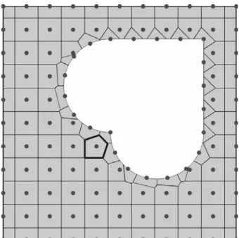
As mentioned above, the inherent flexibility of the meshless FVM enables the use of the Voronoi tessellation for the domain discretization. In mathematics, for a given set of nodes, partitioning of a domain into sub-domains based on distance to the considered nodes called Voronoi tessellation Okabe et al. 2009 . These sub-domains, so called as finite volumes are space-filling polygons in 2D space and can be constructed corresponding to each node by forming the perpendicular bisector lines between the nodes and connecting the lines around each node. A Vo-ronoi tessellation and the local background finite volume associated with an arbitrary node are illustrated in Fig-ure 3.

Figure 3: Voronoi shaped finite volumes. Voronoi tessellation for a given set of nodes dots is illustrated by solid lines and the bold polygon is represented the local background finite volume associated with an arbitrary node.

3.2 Enrichment of approximation space

In order to discretize the governing equations, formulation of the meshless FVM can be used. It satisfies weak form of the balance law over local finite volumes which are formed around the field nodes, see Equation 5 . For a linear elastic solid within the range of infinitesimal deformations, the traction in Equation 5 can be written as follows

i ij j ijkl kl j

t =s n =C e n , 22

where

C

is the 4th _{order elasticity tensor,}

_n

_{is the unit outward normal vector and}

_e

_{is the strain tensor which is} defined as

(

, ,

)

2

kl k l l k

In heterogeneous media that contains material interfaces, enriched approximation space can be applied in order to make domain discretization independent of the material discontinuities; to this end, the enriched ap-proximation Equation 20 is utilized as displacement trial function. In order to obtain the discrete equations, approximated displacement function and its derivatives are needed. The enriched approximation is given as

( )

2

( )

1

( )

( )

1 ˆ 1 1 ˆ

d

n n n

h I I K J K J

i I i J K i

u x =

å

₌ f x u +

å å

_{= =} f s q y r , 24

where

u

ˆ

iI and

ˆ

J K

i

q

_{are the unknown fictitious nodal values for displacement fields and discontinuities amplitude}

parameters. By differentiating this equation one can obtain

( )

2

( )

1

( ) ( )

1

( )

( )

, ₁ , ˆ _{1 1} , ˆ _{1 1} , ˆ

d d

n n n n n

h I I K J J K K J J K

i j I j i J K j i J K j i

u x f x u f s y r q f s y r q

= = = = =

=

å

+

å å

+

å å

25

where _,I j



and _,K j



are the derivatives of 2D and 1D MLS approximation functions, respectively, and J _, j



are derivative of the enrichment approximation functions. Using the chain rule of differentiation

( )

( )

( )

, K K K j j j

s s _s

s

x s x

f f

f = ¶ =¶ ¶

¶ ¶ ¶ , 26

( )

( )

( )

, J J J j j j

r r _r

r

x r x

y y

y = ¶ = ¶ ¶

¶ ¶ ¶ . 27

By substituting Equations 22 - 27 into Equation 5 , finally one obtains the linear algebraic discretized equations for a local finite volume as follows

ˆ

KU =F, 28

where _Uˆ _{is the vector of unknowns,}

K

_and

F

_{are the equivalent local stiffness matrix and load vector,}

respectively, and can be written as follows

0

s su su

K nDBd nDBd Nd

G G G G a G G

= -

_ò

 -

_ò

 -

_ò

, 29

st s su

F td bd ud

G G W W a G G

=

_ò

+

_ò

-

_ò

_{, 30}

where t,

b

and

u

are the prescribed tractions, the body force measured per unit volume and the prescribed displacements, respectively. In Equation 29 ,

D

_{is the elasticity matrix and}

n



_{contains the entries of the unit} outward normal vector and defined as

1 2 2 1 0 0 n n n n n é ù ê ú

= ê_ê ú_ú

ë û

 . 31

Also, the element contribution to

N

and strain–displacement matrix

B

are as follows

I J K

std enr

N = êé_ëN N ù_úû, 32

I J K

std enr

B = êé_ëB B ù_úû, 33

with their entries being

( )

( )

( ) ( )

( ) ( )

0 0

,

0 0

I K J

I J K

std I enr K J

x s r

N N

x s r

f f y

f f y

é ù é ù

ê ú ê ú

= _{ê ú} = _{ê ú}

ê ú ê ú

ë û ë û, 34

( ) ( ) ( ) ( ) ( ) ( ) ( ) ( ) ( ) ( ) ( ) ( ) ( ) ( ) ( ) ( ) ( ) ( ) ( ) ( ) 0 0

,1 ,1 ,1

0 _,2 , 0 _{,2 ,2}

,2 ,1 ,2 ,2 ,1 ,1

I _x K _s J _r K _s J _r

I I J K K J K J

B_std x B_enr s r s r

I _x I _x K _s J _r K _s J _r K _s J _r K _s J _r

f f y f y

f f y f y

f f f y f y f y f y

+

= = +

+ +

é ù é ù

ê ú ê ú

ê ú ê ú

ê ú ê ú

ê ú ê ú

ë û ë û

Accordingly, the vector of unknowns, Uˆ , is expressed as

1 2 1 2

ˆ _ˆI _ˆI J K_ˆ J K_ˆ

U = êé_ëu u q q ù_úû . 36

It should be noted that both

N

_and

B

_{are composed of the standard part and the enriched part, where the}

standard part is computed at every node but the enriched part is only computed at enriched nodes.

Due to the non-polynomial form of the both MLS approximation and enrichment approximation function, ex-act integration of the weak form of the balance law is difficult. So, efficient numerical integration of the weak form may have an important role in the accuracy and computational efficiency of the method Nguyen et al. 2008; Ven-tura et al. 2009 . Hence, weak form of the balance law can be numerically integrated by Gaussian quadrature rule over the finite volumes boundaries. Ventura et al. 2009 have demonstrated that the boundary integration scheme is much more accurate than the domain integration for the same computational cost and it is especially efficient when the integrand has discontinuous and/or non-polynomial form.

3.3 Treatment of additional unknowns

Although in enriched Galerkin-based methods assembling all local equations to the global system leads to as many discrete equations as the number of unknowns, but; the proposed formulation faces to a different situation.

Consider a discretized 2D problem with

n

1 enrichment nodes and

n

2 field nodes. There are two unknown fictitious nodal values associated with every field node and every enrichment node. The unknowns associated with the field nodes are fictitious displacement fields and with the enrichment nodes are fictitious nodal disconti-nuities amplitude parameters. Therefore, the vector of unknowns has

2 n n



1



2



entries. On the other hand, Equation 28 provides two discrete equations for each individual field node or corresponding finite volume, whereas there are no equations corresponding to enrichment nodes, because they have no displacement degrees of freedom. In order to satisfy the momentum balance law over the entire domain, Equation 28 should be ap-plied over all finite volumes. The resulted equations are assembled to form the global system equations. By doing so, we have only

2 n

 

2 discrete equations. This is due to the stack form assembly procedure in finite volume methods.

In order to have the required

2 n

 

1 discrete equations, we need

n

1 additional local finite volumes. Thanks to the inherent flexibilities of the meshless FVM, arbitrarily overlapping local finite volumes can be defined, which resolves this difficulty. To this end, we define

n

1 new local finite volumes corresponding to the selected field nodes. By doing so, Equation 28 provides two additional discrete equations for each newly-defined local finite volume. These equations are independent from the previous set one.

4 NUMERICAL EXPERIMENTS AND RESULTS

In order to assess the performance and accuracy of the proposed formulation, a set of numerical experiments are performed. The considered test problems are linear elastostatic within the range of infinitesimal defor-mations. A one-dimensional bi-material bar and also a two-dimensional infinite plate with a central inclusion both subjected to the prescribed displacement fields are studied. The results are compared with the corresponding solutions obtained by the standard meshless FVM in order to demonstrate the improvements achieved by the proposed formulation. In these experiments, both numerical methods utilized similar domain discretization, but different local approximations. The meshless FVM takes Equation 16 , whereas the proposed formulation takes Equation 20 as displacement trial function. The computations are performed using a domain discretization which is independent of the shape and location of the interface with the appropriate material property at each quadrature point. In order to further highlight the capability of the proposed formulation, some comparisons are also made with the results from the EFG method which has been introduced by Belytschko et al. 1994 .

4.1 1D Bi-material bar

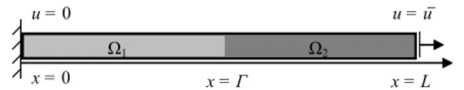
Consider a one-dimensional bar of length L and constant cross sectional area, A, composed of two different materials, i.e.

 

1 2. Young's moduli in

 

1

 

0,



and

  

2

 

,

L

are denoted by

E

1 and

E

2, respec-tively. There is a material discontinuity at

x

 

. The bar is fixed at one end and the other end is subjected to a prescribed displacement

u

. The problem is depicted in Figure 4.

x = L

Ω1

Ω2

x = Γ x = 0

u = 0 u = u

Figure 4: 1D bi-material bar. Problem description. The bar is composed of two different materials, i.e.

 

1 2, with a material discontinuity at

x

 

. The bar is fixed at one end and the other end is subjected to a prescribed

dis-placement

u

.

In the computations, let L 10, A 1,



5,

E

1 1,

E

2 0.5 and

u

1. The computation is performed using 22 uniformly distributed field nodes. One-dimensional finite volumes are constructed with faces located at the middle of the field nodes. In the proposed formulation one enrichment node at the location of the material discontinuity is required. The domain discretization and corresponding finite volumes used in this test are shown in Figure 5. It should be noted that the computations of the EFG method are also performed by using the similar nodal arrangement applied in the standard meshless FVM.

Figure 5: 1D bi-material bar. Domain discretization and corresponding finite volumes. Blue and red dots are denoted the enrichment node and field nodes, respectively. 1D local background finite volumes are illustrated by red lines.

A linear basis and the cubic spline weight function are used in the MLS approximation. The essential bounda-ry conditions are imposed by the penalty method using a value of 1.00E 07 as penalty parameter. The exact ana-lytical solutions for this problem are as follows Krongauz and Belytschko 1998

( )

₍

₎

2

₍

₎

1 2

1 2

5 1

5 5 5

5

E x x

u x

E x E x

E E

ì _£

ïï

= _íï

- + ³

+ _ïî , 37

( )

₍

1 2

₎

1 2

5 E E

x for all x

E E

s =

+ . 38

The nodal displacement and stress values are obtained from the proposed formulation and compared with the exact analytical solutions in Figures 6-7, respectively. In addition, the numerical solutions obtained from the meshless FVM and EFG method are also shown in the same figures for comparison purposes. Figure 6 shows a very good agreement between the nodal displacements obtained from the proposed formulation and the exact analytical solution. In Figure 7, all these numerical methods result in a stress concentration in the vicinity of the material discontinuity. In order to compare local accuracy of these methods, a local relative error norm is defined as the maximum value of





numerical





exact



2

/



exact

Figure 6: 1D bi-material bar. Displacement variation along the bar.

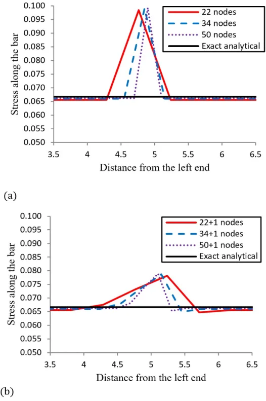
Figure 7: 1D bi-material bar. Stress variation along the bar.

Figure 8: 1D bi-material bar. Convergence results. a Meshless FVM, b Proposed formulation.

In the calculation of error, let

 

num and

 

exact represent approximated and exact analytical solutions, re-spectively. Then, the relative error norms in displacement and stress can be defined as follows

(

)

(

)

2 2

num exact

d

exact

u u d

e

u d

W

W

W

W

-=

ò

ò

, 39

(

)

(

)

2 2

num exact

exact

d e

d

W s

W

s s W

s W

-=

ò

where

u

and



are the displacement and stress at each node, respectively, and



is the computational domain of the bar. Table 1 represents the numerical results for the relative error norms obtained with 50 uniform field nodes and one enrichment node.

Table 1: 1D bi-material bar. The relative error norms.

Error norms Proposed formulation Meshless FVM EFG method

d

e

0.37% 0.38% 0.05%

e

_s 3.12% 6.96% 1.03%

It is clear that both of the proposed formulation and the meshless FVM give almost equal relative error norms in displacement. On the other hand, the proposed formulation yields to a more accurate solution for stress; the relative error norm in stress obtained from the proposed formulation is about half of the meshless FVM result. In addition, both error norms obtained from the EFG method are significantly smaller than those of other meth-ods.

Although in this numerical experiment, the EFG method demonstrates good results, however, it should be mentioned that the observed performance of EFG method is due to the well-adjusted quadrature points which cannot be accommodated in 1D formulation of FV-based methods. It is worth mentioning that in the 1D formula-tion of FV-based methods quadrature points are restricted to be located at two endpoints of each 1D local finite volume. However, as demonstrated, the effect of this drawback has been reduced by the proposed formulation through the enrichment of approximation space.

4.2 2D infinite plate with an inclusion

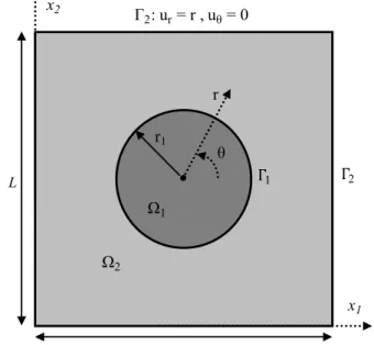
Consider a two-dimensional infinite plate with a circular inclusion subjected to a prescribed displacement field. In the numerical model, a bi-material square domain of length L with a centered circular inclusion of radius

1

r

_{is considered, i.e.}

 

_{1 2. Young's modulus and Poisson's ratio of the inclusion}



_{1 are denoted by}

E

₁

and



1 and those of the matrix



2 are denoted by

E

2 and



2, respectively. There is a material discontinuity across the interface



1

r r



1 where tractions and displacements are continuous across it. The problem is de-picted in Figure 9.

Ω2 

 

Ω₁

r1

θ

r

Γ1

Γ2

Γ2:ur = r ,uθ = 0

x2

x1

L

L

Figure 9: 2D infinite plate with an inclusion. Problem description. The plate is composed of a square domain of length L with a centered circular inclusion of radius

r

1, i.e.

Ω Ω Ω

 

1 2, with a material discontinuity across the interface

Γ

1.

The model is subjected to a prescribed displacement field on the external boundary

Γ

2. In the polar coordinate system, the essential boundary conditions on the external boundary

2

,

0

r

u

=

r u

_q

=

_{. 41}

In the computations, L 2,

r

1 0.4,

E

1 2,



1 0.2,

E

2 10,



2 0.3 and the plane strain state are as-sumed. The computation is made using 452 field nodes. The proposed formulation added 36 enrichment nodes along the line of material discontinuity. The Voronoi tessellation is employed to construct finite volumes. The domain discretization and corresponding finite volumes used in this test are shown in Figure 10. It should be not-ed that similar nodal arrangement usnot-ed in the standard meshless FVM is also utiliznot-ed in the EFG method.

A four-point Gaussian quadrature rule is applied in order to integrate the weak form of governing equation. A quadratic basis, circular domain of influence and the cubic spline weight function are used in the MLS approxima-tion. The essential boundary conditions are imposed by the penalty method using a value of 1.00E 07 as penalty parameter.

a

b

Figure 10: 2D infinite plate with an inclusion. Domain discretization and corresponding finite volumes. Blue and red dots are denoted the enrichment nodes and field nodes, respectively. 1D and 2D local background finite volumes are illustrated by blue and red lines, respectively. Due to symmetry, only a quarter of the domain is shown. a Meshless

FVM, b Proposed formulation.

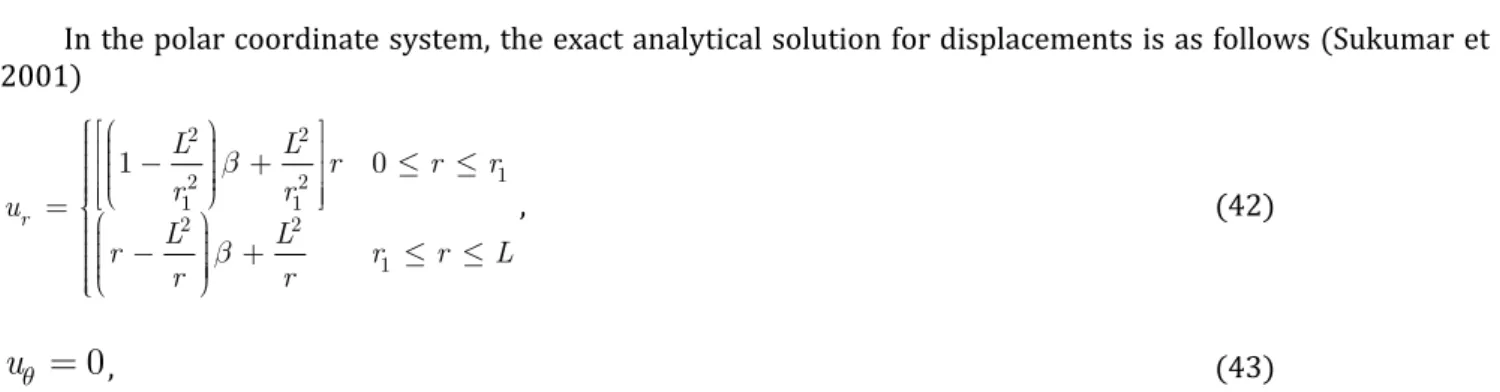
In the polar coordinate system, the exact analytical solution for displacements is as follows Sukumar et al. 2001 2 2 1 2 2 1 1 2 2 1 1 0 r L L

r r r

r r

u

L L

r r r L

r r

b

b

ì éæ ö ù

ï _{ç ÷}

ï êç ÷ ú

ï_êç - ÷ + _ú £ £

ï _ç ÷_÷

ï è ø

ï ê_ë ú_û

= íæï_ïç ö_÷ ÷

ïç - _÷ + £ £

ïç_{ç ÷÷}

ïè ø

ïî

, 42

0

u

_q

=

_{, 43}

and the exact analytical stress fields are given by the following equations where the shear stress field is zero Sukumar et al. 2001 .

(

)

(

)

2 2 1 2 2 1 1 2 2 1 2 2

1 2 2 0

1 2 2

rr

L L

r r

r r

L L

r r L

r r

b m l

s

b m lb

ìéæ ö ù

ï _{ç ÷}

ïêç ÷ ú

ï_êç - _÷ + _ú + £ £

ï _ç ÷_÷

ï è ø

ïê_ë ú_û

= íéæï_{ï çê} ö_÷ ù ú ÷

ï ç + _÷ - + £ £

ï çê_{ç ÷÷} ú

ï èê ø ú

ïîë û

, 44

(

)

(

)

2 2 1 2 2 1 1 2 2 1 2 2

1 2 2 0

1 2 2

L L

r r

r r

L L

r r L

r r

qq

b m l

s

b m lb

ì éæ ö ù

ï _{ç ÷}

ï êç ÷ ú

ï_êç - ÷ + _ú + £ £

ï _ç ÷_÷

ï è ø

ï ê_ë ú_û

= í éæï_{ï çê} ö_÷ ù_ú ÷

ï ç - _÷ + + £ £

ï çê_{ç ÷÷} ú

ï èê ø ú

ïî ë û

, 45

where



_and



are appropriate Lame constants at each material and  is defined as

(

)

(

)

(

)

(

)

2

1 1 2

2 2 2 2

2 2 1 1 1 1 2

L

r L r L

l m m

b

l m l m m

+ +

=

+ + + - + . 46

The analytical solutions for this problem are given in the polar coordinate system, in which they can be trans-formed to the Cartesian coordinate system using equations provided in Appendix A.

The solutions obtained from the proposed formulation, meshless FVM, EFG method and also exact analytical one are shown in Figures 11-12 for the horizontal displacement

u

x and the normal stress



xx both along the

line

y



x

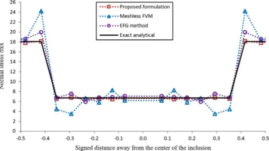
, respectively. A magnified view around the discontinuities is presented in Figure 12 for better observa-tion.

Figure 12: 2D infinite plate with an inclusion. Variation of the



xx along the line

y



x

. A magnified around the

dis-continuities view.

It is clear from Figure 11 that the nodal displacement curve obtained from the proposed formulation agrees well with the exact analytical solution, especially in the vicinity of the material discontinuity. In addition, it is seen in Figure 12 that a significantly higher accuracy in the nodal stress curve is achieved by the proposed formulation as compared with the other meshless methods. The meshless FVM and EFG method fail to reproduce the expected jumps in the nodal stress curve. However, oscillations around the material discontinuity are vanished in the solu-tion obtained from the proposed formulasolu-tion.

Another notable observation is that normal stress



xx is constant within the inclusion. The L2 relative error

norm of the predicted



xx inside the inclusion for meshless FVM and EFG method is 0.012 and 0.008,

respective-ly, while the proposed formulation reduces it to 0.002.

In the calculation of error, the numerical solutions are compared to the exact analytical ones. Let

 

num and

 

exact

represent approximated numerical and exact analytical solutions, respectively, then the relative error norms in displacement and stress could be defined as follows

(

) (

.

)

.

num exact num exact

d

exact exact

u u u u d

e

u u d

W

W

W

W

-

-=

ò

ò

, 47

(

) (

.

)

.

num exact num exact

exact exact

d e

d

W s

W

s s s s W

s s W

-

-=

ò

ò

, 48

where

u

_and

σ

_{are the vectors of displacement and stress at each point, respectively, and}



_{is the}

computational domain of the problem. Table 2 represents the results for the relative error norms. Clearly, proposed formulation yields to more accurate results than both meshless FVM and EFG method.

Table 2: 2D infinite plate with an inclusion. The relative error norms.

Error norms Proposed formulation Meshless FVM EFG method

d

e

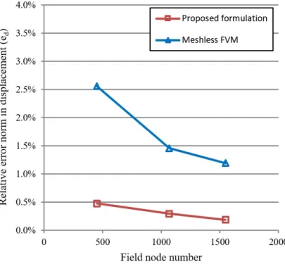
0.48% 2.56% 1.50%

In order to further evaluate the proposed formulation, a convergence study is conducted using 452, 1068 and 1548 field nodes. In the above mentioned tests, the proposed formulation employs 36, 84 and 140 enrichment nodes along the material interface, respectively. Computations of the meshless FVM are carried out using similar field nodes. The numerical results for the relative error norm in displacement predictions are plotted against the field node number in Figure 13.

Figure 13: 2D infinite plate with an inclusion. Convergence results.

The proposed formulation yields to solutions with less error than meshless FVM and the error of the pro-posed formulation falls below 0.2% when the node number increases to 1688 including 1548 field nodes and 140 enrichment nodes .

4.3 2D infinite plate with an extremely soft inclusion

In order to demonstrate the capability of the proposed formulation in the extreme cases, above mentioned two-dimensional infinite plate is considered in a different state regarding to inclusion material property. In this case we let

E

1 0.02 while

E

2 remains equal to 10. Similar geometry, boundary conditions, nodal arrangement and numerical techniques are used as presented in the previous test.

Figure 14: 2D infinite plate with an extremely soft inclusion. Variation of the

u

x along the line

y x



.

Figure 15: 2D infinite plate with an extremely soft inclusion. Variation of the



xx along the line

y



x

. A magnified

around the discontinuities view.

Figure 14 shows a very good agreement between the solution of the proposed formulation and the exact ana-lytical one. The kinks across the material discontinuities are accurately captured. In Figure 15, a magnified view around the discontinuities is presented. As can be seen in Figure 15, while nodal stress curves obtained from meshless FVM and EFG method show oscillations in the vicinity of the material discontinuity, they are alleviated in the proposed formulation results. As mentioned already, the normal stress

σ

xx is constant within the inclu-sion. The L2 relative error norm of the predicted

σ

xx inside the extremely soft inclusion for the meshless FVM, EFG method and proposed formulation are 0.019, 0.024 and 0.001, respectively.

In addition, the results for the relative error norms calculated using Equations 47 - 48 are reported in Ta-ble 3.

Table 3: 2D infinite plate with an extremely soft inclusion. The relative error norms.

Error norms Proposed formulation Meshless FVM EFG method

d

e

0.97% 3.77% 3.23%

e

_s 3.40% 31.09% 7.00%

Figure 16: 2D infinite plate with an extremely soft inclusion. Convergence results.

5 CONCLUSIONS

The aim of this paper is to propose a 2D formulation based on the meshless FVM framework for solving prob-lems with material discontinuity. In order to capture the discontinuity in the gradient fields, the MLS approxima-tion space has been enriched by a continuous funcapproxima-tion, having discontinuity in its derivatives. In contrast to the standard meshless methods, in the proposed formulation, the domain discretization task is done independently of the material discontinuities and also displacement and traction continuity constraints at the interface is automati-cally satisfied without additional treatment. Utilizing enrichment and also space-filling Voronoi-shaped local finite volumes, greatly simplifies the domain discretization task.

Several numerical experiments have been performed. The comparisons with the analytical solutions have shown an excellent agreement in both displacement and stress fields predictions. It has demonstrated that the proposed formulation could alleviate the expecting oscillations in derivative fields in the vicinity of the material discontinuities appeared in the standard meshless methods. The formulation has been also successfully applied to the case of extremely soft inclusion problem. In comparison with the Galerkin-based methods, the proposed for-mulation is particularly attractive as it employs boundary integration over the finite volumes boundaries instead of domain integration. It should be mentioned that, as stated in Ventura et al. 2009 , the boundary integration scheme is much more accurate than the domain integration for the same computational cost and it is especially efficient when the integrand has non-polynomial form.

The results indicate the potential and promise feathers of the proposed formulation for studies of the me-chanics of heterogeneous media.

References

An, X., Ma, G., Cai, Y., Zhu, H. 2011 . A new way to treat material discontinuities in the numerical manifold meth-od. Computer Methods in Applied Mechanics and Engineering, 200 47 : 3296-3308.

Atluri, S., Han, Z., Rajendran, A. 2004 . A new implementation of the meshless finite volume method, through the MLPG “mixed” approach. CMES: Computer Modeling in Engineering & Sciences, 6 6 : 491-513.

Atluri, S.N., Shen, S. 2002 . The Meshless Local Petrov-Galerkin MLPG Method: A Simple\ & Less-costly Alterna-tive to the Finite Element and Boundary Element Methods. CMES: Computer Modeling in Engineering & Sciences, 3 1 : 11-52.

Atluri, S.N., Zhu, T. 1998 . A new meshless local Petrov-Galerkin MLPG approach in computational mechanics. Computational mechanics, 22 2 : 117-127.

Belytschko, T., Black, T. 1999 . Elastic crack growth in finite elements with minimal remeshing. International journal for numerical methods in engineering, 45 5 : 601-620.

Belytschko, T., Krongauz, Y., Organ, D., Fleming, M., Krysl, P. 1996 . Meshless methods: an overview and recent developments. Computer methods in applied mechanics and engineering, 139 1 : 3-47.

Belytschko, T., Lu, Y.Y., Gu, L. 1994 . Element-Free Galerkin Methods. International journal for numerical meth-ods in engineering, 37 2 : 229-256.

Cardiff, P., Karač, A., Ivanković, A. 2014 . A large strain finite volume method for orthotropic bodies with general material orientations. Computer Methods in Applied Mechanics and Engineering, 268 318-335.

Cavalcante, M.A., Marques, S.P., Pindera, M.-J. 2007 . Parametric formulation of the finite-volume theory for func-tionally graded materials—part I: analysis. Journal of Applied Mechanics, 74 5 : 935-945.

Cavalcante, M.A., Pindera, M.-J. 2016 . Generalized FVDAM theory for elastic–plastic periodic materials. Interna-tional Journal of Plasticity, 77 90-117.

Cordes, L., Moran, B. 1996 . Treatment of material discontinuity in the element-free Galerkin method. Computer Methods in Applied Mechanics and Engineering, 139 1 : 75-89.

de Borst, R. 2008 . Challenges in computational materials science: multiple scales, multi-physics and evolving discontinuities. Computational Materials Science, 43 1 : 1-15.

Ebrahimnejad, M., Fallah, N., Khoei, A. 2014 . New approximation functions in the meshless finite volume method for 2D elasticity problems. Engineering Analysis with Boundary Elements, 46 10-22.

Ebrahimnejad, M., Fallah, N., Khoei, A. 2015 . Adaptive refinement in the meshless finite volume method for elas-ticity problems. Computers & Mathematics with Applications, 69 12 : 1420-1443.

Ebrahimnejad, M., Fallah, N., Khoei, A.R. 2017 . Three types of meshless finite volume method for the analysis of two-dimensional elasticity problems. Computational and Applied Mathematics, 36 2 : 971-990.

Escarpini Filho, R.d.S., Marques, S.P.C. 2016 . A model for homogenization of linear viscoelastic periodic compo-site materials with imperfect interface. Latin American Journal of Solids and Structures, 13 14 : 2706-2735.

Fallah, N. 2004 . A cell vertex and cell centred finite volume method for plate bending analysis. Computer meth-ods in applied Mechanics and Engineering, 193 33 : 3457-3470.

Fries, T.-P., Belytschko, T. 2010 . The extended/generalized finite element method: an overview of the method and its applications. International Journal for Numerical Methods in Engineering, 84 3 : 253-304.

Gdoutos, E.E. 2005 . Fracture mechanics: an introduction. Springer Science & Business Media, Netherlands.

Han, Z., Rajendran, A., Atluri, S. 2005 . Meshless Local Petrov-Galerkin MLPG Approaches for Solving Nonlinear Problems with Large Deformations and Rotations. CMES: Computer Modeling in Engineering & Sciences, 10 1 : 1-12.

Hosseini, S.M., Sladek, J., Sladek, V. 2011 . Meshless local Petrov–Galerkin method for coupled thermoelasticity analysis of a functionally graded thick hollow cylinder. Engineering Analysis with Boundary Elements, 35 6 : 827-835.

Krongauz, Y., Belytschko, T. 1998 . EFG approximation with discontinuous derivatives. International Journal for Numerical Methods in Engineering, 41 7 : 1215-1233.

Li, Q., Shen, S., Han, Z., Atluri, S. 2003 . Application of meshless local Petrov-Galerkin MLPG to problems with singularities, and material discontinuities, in 3-D elasticity. Computer Modeling in Engineering and Sciences, 4 5 : 571-586.

Li, S., Hao, W., Liu, W.K. 2000 . Mesh-free simulations of shear banding in large deformation. International Jour-nal of solids and structures, 37 48 : 7185-7206.

Liu, G.-R. 2009 . Meshfree methods: moving beyond the finite element method. CRC Press, Taylor & Francis, Boca Raton.

Liu, G.-R., Gu, Y.-T. 2005 . An introduction to meshfree methods and their programming. Springer Science & Business Media, Netherlands.

Melenk, J.M., Babuška, I. 1996 . The partition of unity finite element method: basic theory and applications. Com-puter methods in applied mechanics and engineering, 139 1 : 289-314.

Moës, N., Cloirec, M., Cartraud, P., Remacle, J.-F. 2003 . A computational approach to handle complex microstruc-ture geometries. Computer methods in applied mechanics and engineering, 192 28 : 3163-3177.

Nguyen, V.P., Rabczuk, T., Bordas, S., Duflot, M. 2008 . Meshless methods: a review and computer implementation aspects. Mathematics and computers in simulation, 79 3 : 763-813.

Okabe, A., Boots, B., Sugihara, K., Chiu, S.N. 2009 . Spatial tessellations: concepts and applications of Voronoi dia-grams. John Wiley & Sons, England.

Sladek, J., Sladek, V., Solek, P., Saez, A. 2008 . Dynamic 3D axisymmetric problems in continuously non-homogeneous piezoelectric solids. International Journal of Solids and Structures, 45 16 : 4523-4542.

Soares, D., Sladek, V., Sladek, J. 2012 . Modified meshless local Petrov–Galerkin formulations for elastodynamics. International Journal for Numerical Methods in Engineering, 90 12 : 1508-1528.

Sukumar, N., Chopp, D.L., Moës, N., Belytschko, T. 2001 . Modeling holes and inclusions by level sets in the ex-tended finite-element method. Computer methods in applied mechanics and engineering, 190 46 : 6183-6200.

Taylor, G., Bailey, C., Cross, M. 2003 . A vertex-based finite volume method applied to non-linear material prob-lems in computational solid mechanics. International journal for numerical methods in engineering, 56 4 : 507-529.

Ventura, G., Gracie, R., Belytschko, T. 2009 . Fast integration and weight function blending in the extended finite element method. International Journal for Numerical Methods in Engineering, 77 1 : 1-29.

Yoon, Y.-C., Song, J.-H. 2014 . Extended particle difference method for weak and strong discontinuity problems: part I. Derivation of the extended particle derivative approximation for the representation of weak and strong discontinuities. Computational Mechanics, 53 6 : 1087-1103.

Appendix A Transformation of field variables

Two-dimensional displacement and stress components in the polar coordinate system can be transformed to the Cartesian coordinate system through the equations provided here. The coordinate systems are illustrated in Figure A.1.

x2

x1 θ

r

Figure A.1: Cartesian and polar coordinate systems.

Displacement transformation

cos

sin

x r

u

=

q

u

-

q

u

_{q A.1}

sin cos

y r

u = qu + qu_{q A.2}

Stress transformation

(

)

(

)

(

)

1

1 cos 2 1 cos 2 2 sin 2

2

x r q rq

s = é_ë + q s + - q s - q s ù_û A.3

(

)

(

)

(

)

1

1 cos 2 1 cos 2 2 sin 2

2

y r q rq

s = é_ë - q s + + q s + q s ù_û A.4

(

)

(

)

(

)

1

sin 2 sin 2 2 cos 2

2

xy r q rq

Erratum

In the article An enriched meshless finite volume method for the modeling of material discontinuity problems in 2D elasticity, doi number: http://dx.doi.org/10.1590/1679-78254121, published in journal Latin American Journal of Solids and Structures, 15(2):e13, page 1:

Where it reads:

Abdullah Davoudi-Kia a

N. Fallah a,b,*

a _{Department of Civil Engineering, University of Guilan, P.O. Box 3756, Rasht, Iran.}

b _{Faculty of Civil Engineering, Babol Noshirvani University of Technology, Babol, Iran.}

davoudikia@phd.guilan.ac.ir *fallah@nit.ac.ir

It should read:

Abdullah Davoudi-Kia a

N. Fallah a,b,*

a _{Department of Civil Engineering, University of Guilan, P.O. Box 3756, Rasht, Iran. E-mail: davoudikia@phd.guilan.ac.ir}

b _{Faculty of Civil Engineering, Babol Noshirvani University of Technology, Babol, Iran. E-mail: fallah@nit.ac.ir}