An algorithm for delineating and extracting hillslopes and hillslope width functions from gridded elevation data

(1)

HESSD

8, 8865–8901, 2011

An algorithm for delineating and extracting hillslopes

P. Noel et al.

Title Page

Abstract Introduction

Conclusions References

Tables Figures

◭ ◮

Back Close

Full Screen / Esc

Printer-friendly Version Interactive Discussion

Discussion

P

a

per

|

Dis

cussion

P

a

per

|

Discussion

P

a

per

|

Discussio

n

P

a

per

|

Hydrol. Earth Syst. Sci. Discuss., 8, 8865–8901, 2011 www.hydrol-earth-syst-sci-discuss.net/8/8865/2011/ doi:10.5194/hessd-8-8865-2011

Hydrology and Earth System Sciences Discussions

This discussion paper is/has been under review for the journal Hydrology and Earth System Sciences (HESS). Please refer to the corresponding final paper in HESS if available.

An algorithm for delineating and

extracting hillslopes and hillslope width

functions from gridded elevation data

P. Noel, A. N. Rousseau, and C. Paniconi

Institut National de la Recherche Scientifique (INRS), Universit é du Qu ébec, Qu ébec, Canada

Received: 27 August 2011 – Accepted: 30 August 2011 – Published: 29 September 2011

Correspondence to: P. Noel (noelphilippe1@gmail.com)

(2)

HESSD

8, 8865–8901, 2011

P. Noel et al.

Title Page

Tables Figures

◭ ◮

Back Close

Full Screen / Esc

Discussion

P

a

per

|

Dis

cussion

P

a

per

|

Discussion

P

a

per

|

Discussio

n

P

a

per

|

Abstract

Subdivision of catchment into appropriate hydrological units is essential to represent rainfall-runoff processes in hydrological modelling. The commonest units used for this purpose are hillslopes (e.g. Fan and Bras, 1998; Troch et al., 2003). Hillslope width functions can therefore be utilised as one-dimensional representation of

three-5

dimensional landscapes by introducing profile curvatures and plan shapes. An algo-rithm was developed to delineate and extract hillslopes and hillslope width functions by introducing a new approach to calculate an average profile curvature and plan shape. This allows the algorithm to be independent of digital elevation model resolution and to associate hillslopes to nine elementary landscapes according to Dikau (1989). This

10

algortihm was tested on two flat and steep catchments of the province of Quebec, Canada. Results showed great area coverage for hillslope width function over individ-ual hillslopes and entire watershed.

1 Introduction

The representation of rainfall-runoff processes in hydrological modeling is highly

de-15

pendent on spatial scale, landscape properties, and other factors (Grayson and Bl ¨oschl, 2000; Beven, 2001). Subdivision of a catchment into appropriately defined and extracted runoffresponse units represents an important first step in hydrological modeling, and the hillslope is vewed as one of the commonest units used for such pur-poses (e.g. Fan and Bras, 1998; Troch et al., 2003). Hillslopes can be defined as either

20

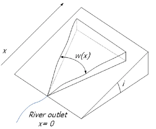
headwater or lateral flow units that encompass the area drained above or to the left or right side of a river segment, respectively (Fig. 1).

The hillslope width function (HWF) is defined as the width of the hillslope from the divide to the river segment. The direction along the transect begins at the river seg-ment and increase to the divide (see Fig. 2 and Sect. 2.3 for further details). HWFs

25

(3)

HESSD

8, 8865–8901, 2011

P. Noel et al.

Title Page

Tables Figures

◭ ◮

Back Close

Full Screen / Esc

Discussion

P

a

per

|

Dis

cussion

P

a

per

|

Discussion

P

a

per

|

Discussio

n

P

a

per

|

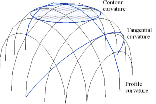
three-dimensional (3-D) landscape of a given hydrological unit into a one-dimensional (1-D) representation (Fan and Bras, 1998; Troch et al., 2003). By introducing profile curvature and plan shape, the HWF can, by its 1-D width variation, illustrate conver-gent, diverconver-gent, and uniform hillslope shapes as well as concave, convex, and straight profiles. Plan shape is defined as the tangential curvature that is perpendicular to the

5

slope gradient while profile curvature refers to the rate of change of slope (Schmidt et al., 2003).

To calculate profile curvature and plan shape most terrain analysis software uses a quadratic equation on a 3×3 matrix as proposed by Zevenbergen and Thorne (1987).

However, this method was found to show higher sensitivity to local variations in input

10

data and digital elevation model (DEM) resolution, leading to greater scatter in spatial patterns of curvature especially for flatter areas (Schmidt et al., 2003). This leads to overestimation of some features within a hillslope and to DEM resolution effects on the profile curvature and plan shape. Thus, there is a need to develop a method that is able to calculate the average plan shape and profile curvature independently of DEM

15

resolution.

Whereas several terrain analysis algorithms are able to extract the principal geomor-phologic characteristics of catchments, such as slope, topographic index, and over-land flow paths (e.g. TARDEM/TauDEM (Tarboton, 1997), TAPES (Moore et al., 1993; Gallant and Wilson, 1996), LandSerf (Woods et al., 1995), LANDLORD (Florinsky et

20

al., 2002), TAS (Lindsay, 2005), LANDFORM (Klingseisen et al., 2008), PHYSITEL (Rousseau et al., 2011) the delineation of hillslopes, including extracting the width func-tion and taking into account plan shape and profile characteristics, is still an unresolved problem (Bogaart and Troch, 2006).

In this paper, a method to delineate hillslopes and extract the width function is

pre-25

(4)

HESSD

8, 8865–8901, 2011

P. Noel et al.

Title Page

Tables Figures

◭ ◮

Back Close

Full Screen / Esc

Discussion

P

a

per

|

Dis

cussion

P

a

per

|

Discussion

P

a

per

|

Discussio

n

P

a

per

|

final hillslope shape according to various criteria. These steps were coded up as an algorithm implemented in PHYSITEL (Rousseau et al., 2010a, b, c), a geographic in-formation system (GIS)-based pre-processor for the HYDROTEL (Fortin et al., 2001; Turcotte et al., 2003) distributed hydrological model.

2 Methodology

5

2.1 Delineation of hillslopes

DEMs contain all the information required for partitioning a river basin into subbasins and for delineating the river network (Orlandini et al., 2003). From this analysis, a flow direction matrix is created that gives the direction of the flow for each cell (or pixel) according to the steepest descent direction, and a flow accumulation matrix is

10

calculated that identifies the upstream grid cell number that flows into each cell. This standard procedure for extracting subbasins, together with the information it encodes in the river network, flow direction, and flow accumulation matrices, is the starting point for further refinement of the DEM into hillslopes. Essentially, for each subbasin, the area drained by the first pixel of the river segment is designated as a

15

headwater hillslope, while the remaining area defines two lateral hillslopes, one on either side of the river segment (Fig. 1).

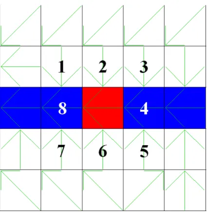
To simplify the analysis, the algorithm considers only those pixels with a flow direc-tion directly towards a current river cell; in so doing the area drained on either side of the river segment can be easily computed. To get these pixels, the algorithm takes as

20

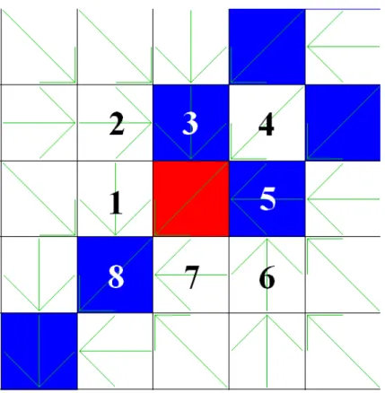
arguments the previous, current, and next river cells. Then, from the flow direction ma-trix, the eight neighbor cells of the current cell are considered (Fig. 4), in clockwise and counterclockwise directions, until the algorithm finds the next or previous river segment cell. Every cell with flow direction directly towards the current cell is retained and put in one of two tables, right or left for, respectively, the clockwise and counterclockwise

25

(5)

HESSD

8, 8865–8901, 2011

P. Noel et al.

Title Page

Tables Figures

◭ ◮

Back Close

Full Screen / Esc

Discussion

P

a

per

|

Dis

cussion

P

a

per

|

Discussion

P

a

per

|

Discussio

n

P

a

per

|

algorithm arrives at an intersection of two or more river segments, it can occur that a cell falls into both tables. To resolve this conflict, it was decided, without loss of con-sistency or generality, to assign such cells to the right table for the river segment in question (see for example cell 4 in Fig. 5 and also the resulting delineation shown in Fig. 6). Once every river segment of the network matrix has been scanned, the table

5

for each specific river segment identifies all the cells that will drain the hillslope (Fig. 6). Finally, the algorithm redraws the hilllsope matrix. Figure 7 summarizes the algorithm for the hillslope delineation process, while Fig. 8 illustrates di_fferent steps of the proce-dure as applied to the des Anglais watershed example that will be presented in more detail in Sect. 3.

10

2.2 Determination of plan shape and profile curvature

Once all hillslopes in a watershed have been delineated, characterization of the plan shape and profile curvature represents the next step. The plan shape corresponding to elevation lines taken parallel to the average flow direction for a given river segment is calculated using the DEM. To characterize an elevation line as convergent, divergent,

15

or uniform, a straight reference line is drawn between the first and last cells of that elevation line. An elevation line is then designated as convergent if the majority of its cells falls far enough below the reference line, divergent if its cells fall far enough above the reference line, and uniform otherwise (Fig. 9). An arbitrary value of 1 m was set to qualify as far enough in the algortihm. However, the user may enter another value

ac-20

cording to the precsion of the DEM. A value of 5 m was used for the examples reported in this study representing the accuracy on the elevation. When all the elevation lines have been processed, a convexity ratio is calculated for each hillslope as the number of convergent elevation lines relative to the total number of lines.

An analogous procedure is used to characterize the profile curvature, with the

ele-25

(6)

HESSD

8, 8865–8901, 2011

P. Noel et al.

Title Page

Tables Figures

◭ ◮

Back Close

Full Screen / Esc

Discussion

P

a

per

|

Dis

cussion

P

a

per

|

Discussion

P

a

per

|

Discussio

n

P

a

per

|

reference line, and straight otherwise. The same precision value as in the plan shape analysis is used. When all the elevation lines have been processed, a convexity ratio is calculated for each hillslope as the number of convex elevation lines relative to the total number of lines.

The resulting convexity percentage ratios for the plan shape and the profile

curva-5

ture, respectively, are then used as inputs to a fuzzy logic algorithm to determine mem-bership in one of the nine elementary landform classes described by (Fig. 10; Dikau, 1989). The input and output membership functions are shown in Fig. 11 and the rule matrix is given in Table 1. The algorithm was tested on theoretical three-dimensional forms.

10

2.3 Extraction of hillslope width functions

Two criteria were applied in the final step of the algorithm for delineating hillslopes and extracting width functions: monotonicity of the HWF and conservation of surface area. The first criterion is imposed in view of the potential application of the algorithm as a pre-processing step for the hillslope-storage Boussinesq model (Paniconi et al., 2003).

15

This hydrological model requires that the width function be monotonically increasing (convergent plan shape), monotonically decreasing (divergent plan shape), or con-stant (uniform shape) in order to avoid flow singularities along the lateral boundaries of the hillslope. The second criterion, applied to individual hillslopes and to the overall watershed, provides a measure of mass conservation when the resulting hillslopes are

20

used in watershed-scale, rainfall-runo_ffmodeling applications.

(7)

HESSD

8, 8865–8901, 2011

P. Noel et al.

Title Page

Tables Figures

◭ ◮

Back Close

Full Screen / Esc

Discussion

P

a

per

|

Dis

cussion

P

a

per

|

Discussion

P

a

per

|

Discussio

n

P

a

per

|

2.3.1 Lateral hillslopes

Figure 12 illustrates the procedure for HWF extraction in the case of lateral hillslopes. The first segment (AD) of the quadrilateral is defined as a line connecting the first and last cells of the river segment and parallel to the average flow direction in the river. Points B and C are then defined by following the boundary cells on the left and right

5

sides, respectively. The algorithm preserves monotonicity and counts the number of hillslope cells inside the quadrilateral. An optimization algorithm is then used to match the original surface area of the hillslope as closely as possible. This algorithm adjusts the position of points B′_{and C}′_{according to the slope defined by the segments AB and}

DC. This will increase or decrease the hillslope surface area (see Fig. 12). The relative

10

accuracy in terms of the second criterion is calculated as follows:

relative precision (%) =modelled surface - actual surface

actual surface ×100 (1)

A new vector is created with the coordinates of the four points that correspond to the quadrilateral vertices. This vector is then used to calculate the width of the hillslope from the divide to the river segment at an increment equal to the DEM cell size. The

15

HWF is exported as a text file that contains, for each hillslope, the distance from the river segment to the divide and the width at the divide. The HWF extraction algorithm for lateral hillslopes is summarized in Fig. 13.

2.3.2 Headwater hillslopes

Figure 14 illustrates the procedure for HWF extraction in the case of headwater

hill-20

slopes, which are always convergent. With point A coincident with the river cell, the triangle is oriented in a way that best respects the general flow direction within the ac-tual hillslope. The algorithm then starts at point A and examines the next cells on the left and right sides, proceeding upslope until the number of cells inside the triangle ex-ceeds the number of cells in the original hillslope. The last two cells examined then get

(8)

HESSD

8, 8865–8901, 2011

P. Noel et al.

Title Page

Tables Figures

◭ ◮

Back Close

Full Screen / Esc

Discussion

P

a

per

|

Dis

cussion

P

a

per

|

Discussion

P

a

per

|

Discussio

n

P

a

per

|

designated as points B and C. Analogously to the lateral hillslope case, an optimization algorithm is applied to adjust points B′ _{and C}′_{, a relative accuracy is calculated, and}

the extracted information is exported as a text file.

3 Application

3.1 Description of the study catchments

5

The Chateauguay River, a tributary ofthe St. Lawrence River, drains a 2500-km2 trans-boundary territory that lies 57 % within the province of Quebec (Canada) and 43 % within the state of New York (USA) (C ˆot ´e et al., 2006). The des Anglais watershed is the largest subcatchment of the Chateauguay River watershed and has a land cover that is predominantly forest in the south and agricultural to the north. The watershed

10

has a drainage area of 690 km2, an average annual discharge of 300×106m3, and an

elevation range from 30 m to 400 m (Sulis et al., 2010). The aquifer system in this region is part of the St. Lawrence Lowlands and consists of Cambrian to Middle Ordovician sedimentary rocks that are slightly deformed and fractured. Unconsolidated sediments of glacial and post-glacial origin overlay the bedrock aquifer and are of varying

thick-15

ness, reaching 40 m in the northernmost portion (Tremblay, 2006). These sediments are in turn overlain by Quaternary deposits of silty till and soils that are characterized as mainly weathered Quaternary sediments (Lamontagne, 2005), with the exception of bogs and swamps that overly Champlain sea sediments in the northeastern part of the catchment. The climate is characterized as semi-humid with a mean annual

tempera-20

ture of 6.3◦_{C and an average annual precipitation of 958 mm (Canadian Daily Cilmate}

Data, 2004). The DEM used for our analysis has a 90-m horizontal resolution and a 5-m vertical resolution and consists of 497×592 cells. The projection is Universal

Transversal Mercator (NAD 83) zone 18.

The second catchment selected for analysis is the “Bassin exp ´erimental du ruisseau

25

(9)

HESSD

8, 8865–8901, 2011

P. Noel et al.

Title Page

Tables Figures

◭ ◮

Back Close

Full Screen / Esc

Discussion

P

a

per

|

Dis

cussion

P

a

per

|

Discussion

P

a

per

|

Discussio

n

P

a

per

|

north of Quebec City. It is part of the Montmorency forest in the high hills of the Lau-rentian mountain chain and has a land cover composed principally of balsam fir with some black and white spruce and white birch. High hills dominate the landscape and the elevation ranges between 990 m and 560 m. The surface geology is composed of glacial and fluvio-glacial tills of depth between 0 and 18 m. The underlying formation

5

is a crystalline mother rock of Precambrian origin composed of charnockitic gneiss. The organic litter has an average thickness of 8 cm and the root depth is 30 cm on average in a podzol ferrohumic soil. This soil layer is very permeable compared to the underlying till and very rapid shallow subsurface flow is often observed. The BEREV catchment discharges into the Montmorency River (Lavigne, 2007). The DEM used for

10

our analysis has a 5 m horizontal resolution and 5 m vertical resolution and consists of 825×799 cells. The projection is Quebec modified Transversal Mercator (NAD 83)

zone 7.

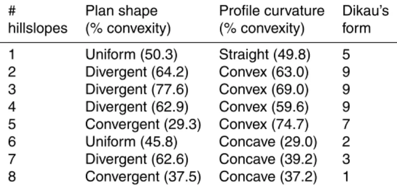
3.2 Results

The proposed algorithm was used to subdivide the des Anglais and BEREV

water-15

sheds into three and eight hillslopes, respectively (Figs. 15 and 16). The extracted plan shapes and profile curvatures are presented in Tables 2 and 3. Figures 15 and 16 illus-trate, visually, the match between the original and extracted hillslope width functions. A more quantitative assessment is provided in Tables 2 and 3, where the resulting con-vexity ratios for plan shape and profile curvature indicate that 2 out of 3 of des Anglais

20

hillslopes represent a flat area and most of the BEREV hillslopes represent an overall steep watershed. Tables 2 and 3 also give the elementary landform class (Fig. 10) attributed to each extracted hillslope according to the rule matrix of Table 1. These results indicate that the algorithm provides the correct Dikau’s form according to the linguistic variable and the rule matrix.

25

(10)

HESSD

8, 8865–8901, 2011

P. Noel et al.

Title Page

Tables Figures

◭ ◮

Back Close

Full Screen / Esc

Discussion

P

a

per

|

Dis

cussion

P

a

per

|

Discussion

P

a

per

|

Discussio

n

P

a

per

|

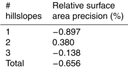
0.180 %. The individual hillslopes also conserved surface area very well, with the highest error reaching only 1.019 % for one of the hillslopes of the BEREV watershed. These results also show that divergent plan shapes lead to HWF that are generally less representative of the surface area because of the limit imposed by the trapezoidal form.

5

Tables 6 and 7 present the plan shape and profile curvature convexity percentages and elementary landform classification with an arbitrary resolution on elevation data of 1 m instead of 5 m for the des Anglais and BEREV watershed respectively. Comparing these results with those of Tables 2 and 3, we note that the convexity ratio is closer to 0.5, affecting even the elementary landform classification of des Anglais hillslope No. 2.

10

So, imprecision on elevation data tends to flatten the plan shape, profile curvature and elementary landform classification.

4 Conclusions

This paper described the development of algorithms to delineate and extract hillslopes and hillslope width functions from gridded elevation data. These algorithms were

ap-15

plied on the des Anglais and the BEREV watersheds, Quebec, Canada. Some rela-tively important problems were encountered with the utilisation of this algorithm over a flat watershed such as the des Anglais. When rivers are too sinous or two or more pix-els wide, the algorithm has some difficulties to find the countour cells. Other problems concern the intersection of two or more rivers that converge into one single river.

How-20

ever, sometimes it is possible to solve some of these issues by changing directions of some cells in the flow accumulation matrix. This lead to small changes in the limits of hillslopes and often helps the algorithm to work properly. Further work still need to be done to increase the robustness of the algortihm to such diificulties. As well, this pro-posed methodology needs to be tested and applied in a hydrological modelling context.

25

(11)

HESSD

8, 8865–8901, 2011

P. Noel et al.

Title Page

Tables Figures

◭ ◮

Back Close

Full Screen / Esc

Discussion

P

a

per

|

Dis

cussion

P

a

per

|

Discussion

P

a

per

|

Discussio

n

P

a

per

|

model (e.g. CATHY, Camporese et al., 2009), over a single or multiple-hillslope basis. This will lead to an assessment of the adequacy of some of the choices and approxima-tions made in the algorithm (flow direction, plan shape, profile curvature, elementary form classification, used of simple geometric form as HWF, etc.), of some of the fun-damentals hypotheses (e.g. monotonicinity), and of the guiding criteria (conservation

5

of area). Also, it could be interesting to compare results of a hydrological model (e.g. HYDROTEL, Fortin et al., 2001; Turcotte et al., 2003, 2007) run on its “standard” dis-cretization of a watershed (into sub-watershed) and run on a disdis-cretization based on the hillslopes derived from the algorithm presented here. This second set of steps can begin to address some of the pros and cons of passing from a “sub-watershed” to a

10

“hillslope”-based discretization and conceptualization of a watershed.

Acknowledgements. This work was supported in part by the Natural Sciences and Engineering Research Council of Canada (NSERC). The authors thank Alain Royer of the Institut National de la Recherche Scientifique, Centre Eau, Terre et Environnement, for his expertise in pro-gramming some of the C++code in PHYSITEL.

15

References

Beven, K. J.: Rainfall-RunoffModelling: The Primer, John Wiley & Sons, New York, 2001. Bogaart, P. W. and Troch, P. A.: Curvature distribution within hillslopes and catchments and its

e_ffect on the hydrological response, Hydrol. Earth Syst. Sci., 10, 925–936, doi:10.5194/hess-10-925-2006, 2006.

20

Camporese, M., Paniconi, C., Putti, M., and Salandin, P.: Ensemble Kalman filter data assim-ilation for a process-based catchment scale model of surface and subsurface flow, Water Resour. Res., 45, W10421, doi:10.1029/2008wr007031, 2009.

Canadian Daily Climate Data (CDCD): available at: http://climate.weatheroffice.ec.gc.ca, last access: 5 September 2010, 2004.

25

(12)

HESSD

8, 8865–8901, 2011

P. Noel et al.

Title Page

Tables Figures

◭ ◮

Back Close

Full Screen / Esc

Discussion

P

a

per

|

Dis

cussion

P

a

per

|

Discussion

P

a

per

|

Discussio

n

P

a

per

|

Environnement, Qu ébec: minist ère du D éveloppement durable, de l’Environnement et des Parcs, 64 pp., 2006.

Dikau, R.: The application of a digital relief model to landform analysis in geomorphology, Three dimensional applications in GIS, 51–77, 1989.

Fan, Y. and Bras, R. L.: Analytical solutions to hillslope subsurface storm flow and saturation

5

overland flow, Water Resour. Res., 34, 921–927, 1998.

Florinsky, I. V., Eilers, R. G., Manning, G. R., and Fuller, L. G.: Prediction of soil proper-ties by digital terrain modelling, Environ. Modell. Softw., 17, 295–311, doi:10.1016/s1364-8152(01)00067-6, 2002.

Fortin, J. P., Turcotte, R., Massicotte, S., Moussa, R., Fitzback, J., and Villeneuve, J. P.:

Dis-10

tributed watershed model compatible with remote sensing and GIS data, I: Description of model, J. Hydrol. Eng., 6, 91–99, doi:10.1061/(asce)1084-0699(2001)6:2(91), 2001.

Gallant, J. C. and Wilson, J. P.: TAPES-G: A grid-based terrain analysis program for the en-vironmental sciences, Comput. Geosci., 22, 713–722, doi:10.1016/0098-3004(96)00002-7, 1996.

15

Grayson, R., and Bl ¨oschl, G.: Spatial Patterns in Catchment Hydrology: Observations and Modelling, Cambridge University Press, Cambridge, 2000.

Klingseisen, B., Metternicht, G., and Paulus, G.: Geomorphometric landscape anal-ysis using a semi-automated GIS-approach, Environ. Modell. Softw., 23, 109–121, doi:10.1016/j.envsoft.2007.05.007, 2008.

20

Lamontagne, L.: Base de donn ées sur les propri ét és physiques des sols du bassin versant de la rivi ère Ch âteauguay, Pedology and Precision Agriculture Laboratories, Agriculture and Agri-Food Canada, QC, CD-Rom, 2005.

Lavigne, M.-P.: Mod élisation du r égime hydrologique et de l’impact des coupes foresti ères sur l’ écoulement du ruisseau des Eaux-Vol ées à l’aide d’Hydrotel, Water sciences master,

25

Water sciences, Institut national de la recherche scientifique – Eau, Terre et Environnement, Qu ´ebec, 267 pp., 2007.

Lindsay, J. B.: The Terrain Analysis System: A tool for hydro-geomorphic applications, Hydrol. Process., 19, 1123–1130, doi:10.1002/hyp.5818, 2005.

Moore, I. D., Gallant, J. C., Guerra, L., and Kalma, J. D.: Modelling the spatial variability of

hy-30

(13)

HESSD

8, 8865–8901, 2011

P. Noel et al.

Title Page

Tables Figures

◭ ◮

Back Close

Full Screen / Esc

Discussion

P

a

per

|

Dis

cussion

P

a

per

|

Discussion

P

a

per

|

Discussio

n

P

a

per

|

Orlandini, S., Moretti, G., Franchini, M., Aldighieri, B., and Testa, B.: Path-based methods for the determination of nondispersive drainage directions in grid-based digital elevation models, Water Resour. Res., 39, 1144, doi:10.1029/2002WR001639, 2003.

Paniconi, C., Troch, P. A., Van Loon, E. E., and Hilberts, A. G. J.: Hillslope-storage Boussinesq model for subsurface flow and variable source areas along complex hillslopes: 2.

Intercom-5

parison with a three-dimensional Richards equation model, Water Resour. Res., 39(11), 1317, doi:10.1029/2002WR001730, 2003.

Rousseau, A. N., Fortin, J.-P., Turcotte, R., Royer, A., Savary, S., Qu ´evy, F., No ¨el, P., and Paniconi, C.:: PHYSITEL, a specialized GIS for supporting the implementation of distributed hydrological models, Water News, Official Magazine of CWRA – Canadian Water Resources

10

Association, 31, 18–20, 2011.

Schmidt, J., Evans, I. S., and Brinkmann, J.: Comparison of polynomial mod-els for land surface curvature calculation, Int. J. Geogr. Inf. Sci., 17, 797–814, doi:10.1080/13658810310001596058, 2003.

Sulis, M., Paniconi, C., Rivard, C., Harvey, R., and Chaumont, D.: Assessment of

cli-15

mate change impacts at the catchment scale with a detailed hydrological model of sur-face/subsurface interactions, and comparison with a land surface model, Water Resour. Res., 47, W01513, doi:10.1029/2010WR009167, 2010.

Tarboton, D. G.: A new method for the determination of flow directions and upslope areas in grid digital elevation models, Water Resour. Res., 33, 309–319, 1997.

20

Tremblay, T.: Hydrostratigraphie et g éologie du Quaternaire dans le bassin-versant de la rivi ère Ch âteauguay, Qu ébec, Master, UQAM, Montr éal, 2006.

Troch, P. A., Paniconi, C., and Van Loon, E. E.: Hillslope-storage Boussinesq model for subsur-face flow and variable source areas along complex hillslopes: 1. Formulation and character-istic response, Water Resour. Res., 39, 1316, doi:10.1029/2002WR001728, 2003.

25

Turcotte, R., Fortin, J.-P., Rousseau, N. A., Massicotte, S., and Villeneuve, J. P.: Determination of the drainage structure of a watershed using a digital elevation model and a digital river and lake network, J. Hydrol., 240, 225–242, 2001.

Turcotte, R., Rousseau, N. A., Fortin, J. P., and Villeneuve, J. P.: A process-oriented multiple-objective calibration strategy accounting for model structure, in: Calibration of watershed

30

models, edited by: Duan, Q., Gupta, V. K., Sorooshian, S., Rousseau, A. N., and Turcotte, R., American Geophysical Union, Washington, 153–163, 2003.

(14)

HESSD

8, 8865–8901, 2011

P. Noel et al.

Title Page

Tables Figures

◭ ◮

Back Close

Full Screen / Esc

Discussion

P

a

per

|

Dis

cussion

P

a

per

|

Discussion

P

a

per

|

Discussio

n

P

a

per

|

of the spatial distribution and the temporal evolution of the snowpack water equivalent in southern Qu ´ebec, Canada, Nordic Hydrol., 38, 211–234, doi:10.2166/nh.2007.009, 2007. Woods, R., Sivapalan, M., and Duncan, M.: Investigating the representative elementary area

concept: an approach based on field data, Hydrol. Process., 9, 291–312, 1995.

Zevenbergen, L. W. and Thorne, C. R.: Quantitative analysis of land surface topography, Earth

5

(15)

HESSD

8, 8865–8901, 2011

P. Noel et al.

Title Page

Tables Figures

◭ ◮

Back Close

Full Screen / Esc

Discussion

P

a

per

|

Dis

cussion

P

a

per

|

Discussion

P

a

per

|

Discussio

n

P

a

per

|

Table 1.Fuzzy rule matrix.

IF

THEN Curvature/shape

Profile Plan Form

Concave Divergent 1

Concave Uniform 2

Concave Convergent 3 Straight Divergent 4

Straight Uniform 5

Straight Convergent 6 Convexe Divergent 7

Convexe Uniform 8

(16)

HESSD

8, 8865–8901, 2011

P. Noel et al.

Title Page

Tables Figures

◭ ◮

Back Close

Full Screen / Esc

Discussion

P

a

per

|

Dis

cussion

P

a

per

|

Discussion

P

a

per

|

Discussio

n

P

a

per

|

Table 2. Plan shapes and profile curvatures for each hillslope of the des Anglais watershed and associated Dikau’s form.

# Plan shape Profile curvature Dikau’s

hillslopes (% convexity) (% convexity) form

1 Convergent (24.2) Concave (39.1) 1

2 Uniform (52.0) Straight (53.2) 5

(17)

HESSD

8, 8865–8901, 2011

P. Noel et al.

Title Page

Tables Figures

◭ ◮

Back Close

Full Screen / Esc

Discussion

P

a

per

|

Dis

cussion

P

a

per

|

Discussion

P

a

per

|

Discussio

n

P

a

per

|

Table 3. Plan shapes and profile curvatures for each hillslope of the BEREV watershed and associated Dikau’s form.

2 Divergent (64.2) Convex (63.0) 9

5 Convergent (29.3) Convex (74.7) 7

6 Uniform (45.8) Concave (29.0) 2

7 Divergent (62.6) Concave (39.2) 3

(18)

HESSD

8, 8865–8901, 2011

P. Noel et al.

Title Page

Tables Figures

◭ ◮

Back Close

Full Screen / Esc

Discussion

P

a

per

|

Dis

cussion

P

a

per

|

Discussion

P

a

per

|

Discussio

n

P

a

per

|

Table 4.Relative surface area precision obtained for each HWF of the des Anglais watershed.

# Relative surface

hillslopes area precision (%)

1 −0.897

2 0.380

3 −0.138

(19)

HESSD

8, 8865–8901, 2011

P. Noel et al.

Title Page

Tables Figures

◭ ◮

Back Close

Full Screen / Esc

Discussion

P

a

per

|

Dis

cussion

P

a

per

|

Discussion

P

a

per

|

Discussio

n

P

a

per

|

Table 5. Relative surface area precision obtained for each HWF of the BEREV watershed.

# Relative surface

hillslopes area precision (%)

1 −0.401

2 −0.363

3 −0.256

4 −0.037

5 −0.214

6 −0.006

7 1.019

8 0.079

(20)

HESSD

8, 8865–8901, 2011

P. Noel et al.

Title Page

Tables Figures

◭ ◮

Back Close

Full Screen / Esc

Discussion

P

a

per

|

Dis

cussion

P

a

per

|

Discussion

P

a

per

|

Discussio

n

P

a

per

|

Table 6. Plan shapes and profile curvatures for each hillslope of the des Anglais watershed and associated Dikau’s form with a 1-m resolution on elevation data.

1 Convergent (17.3) Concave (33.3) 1

(21)

HESSD

8, 8865–8901, 2011

P. Noel et al.

Title Page

Tables Figures

◭ ◮

Back Close

Full Screen / Esc

Discussion

P

a

per

|

Dis

cussion

P

a

per

|

Discussion

P

a

per

|

Discussio

n

P

a

per

|

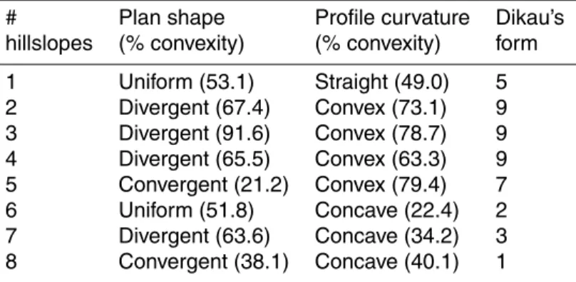
Table 7. Plan shapes and profile curvatures for each hillslope of the BEREV watershed and associated Dikau’s form with a 1-m resolution on elevation data.

5 Convergent (21.2) Convex (79.4) 7

6 Uniform (51.8) Concave (22.4) 2

7 Divergent (63.6) Concave (34.2) 3

(22)

HESSD

8, 8865–8901, 2011

P. Noel et al.

Title Page

Tables Figures

◭ ◮

Back Close

Full Screen / Esc

Discussion

P

a

per

|

Dis

cussion

P

a

per

|

Discussion

P

a

per

|

Discussio

n

P

a

per

|

(23)

HESSD

8, 8865–8901, 2011

P. Noel et al.

Title Page

Tables Figures

◭ ◮

Back Close

Full Screen / Esc

Discussion

P

a

per

|

Dis

cussion

P

a

per

|

Discussion

P

a

per

|

Discussio

n

P

a

per

|

(24)

HESSD

8, 8865–8901, 2011

P. Noel et al.

Title Page

Tables Figures

◭ ◮

Back Close

Full Screen / Esc

Discussion

P

a

per

|

Dis

cussion

P

a

per

|

Discussion

P

a

per

|

Discussio

n

P

a

per

|

(25)

HESSD

8, 8865–8901, 2011

P. Noel et al.

Title Page

Tables Figures

◭ ◮

Back Close

Full Screen / Esc

Discussion

P

a

per

|

Dis

cussion

P

a

per

|

Discussion

P

a

per

|

Discussio

n

P

a

per

|

(26)

HESSD

8, 8865–8901, 2011

P. Noel et al.

Title Page

Tables Figures

◭ ◮

Back Close

Full Screen / Esc

Discussion

P

a

per

|

Dis

cussion

P

a

per

|

Discussion

P

a

per

|

Discussio

n

P

a

per

|

(27)

HESSD

8, 8865–8901, 2011

P. Noel et al.

Title Page

Tables Figures

◭ ◮

Back Close

Full Screen / Esc

Discussion

P

a

per

|

Dis

cussion

P

a

per

|

Discussion

P

a

per

|

Discussio

n

P

a

per

|

(28)

HESSD

8, 8865–8901, 2011

P. Noel et al.

Title Page

Tables Figures

◭ ◮

Back Close

Full Screen / Esc

Discussion

P

a

per

|

Dis

cussion

P

a

per

|

Discussion

P

a

per

|

Discussio

n

P

a

per

|

With accumulation matrix and river network matrix.

while (current cell != river network last cell – 1)

if current cell == first river network segment cell

associate headwater hillslope with cells drained by river network current cell

end

else

With previous, current and next river cell

Clockwise :

if neighbor cell != river segment cell

if neighbor cell flow direction == toward current cell

add neighbor cell to right table

end

neighbor cell = neighbor cell + 1

end

Counterclockwise

If neighbor cell != river segment cell

if neighbor cell flow direction == toward current cell

add neighbor cell to left table

end

neighbor cell = neighbor cell + 1

end

previous cell = river network previous cell + 1

current cell = river network current cell + 1

next cell = river network next cell + 1

end

(29)

HESSD

8, 8865–8901, 2011

P. Noel et al.

Title Page

Tables Figures

◭ ◮

Back Close

Full Screen / Esc

Discussion

P

a

per

|

Dis

cussion

P

a

per

|

Discussion

P

a

per

|

Discussio

n

P

a

per

|

(30)

HESSD

8, 8865–8901, 2011

P. Noel et al.

Title Page

Tables Figures

◭ ◮

Back Close

Full Screen / Esc

Discussion

P

a

per

|

Dis

cussion

P

a

per

|

Discussion

P

a

per

|

Discussio

n

P

a

per

|

(31)

HESSD

8, 8865–8901, 2011

P. Noel et al.

Title Page

Tables Figures

◭ ◮

Back Close

Full Screen / Esc

Discussion

P

a

per

|

Dis

cussion

P

a

per

|

Discussion

P

a

per

|

Discussio

n

P

a

per

|

(32)

HESSD

8, 8865–8901, 2011

P. Noel et al.

Title Page

Tables Figures

◭ ◮

Back Close

Full Screen / Esc

Discussion

P

a

per

|

Dis

cussion

P

a

per

|

Discussion

P

a

per

|

Discussio

n

P

a

per

|

(33)

HESSD

8, 8865–8901, 2011

P. Noel et al.

Title Page

Tables Figures

◭ ◮

Back Close

Full Screen / Esc

Discussion

P

a

per

|

Dis

cussion

P

a

per

|

Discussion

P

a

per

|

Discussio

n

P

a

per

|

(34)

HESSD

8, 8865–8901, 2011

P. Noel et al.

Title Page

Tables Figures

◭ ◮

Back Close

Full Screen / Esc

Discussion

P

a

per

|

Dis

cussion

P

a

per

|

Discussion

P

a

per

|

Discussio

n

P

a

per

|

(35)

HESSD

8, 8865–8901, 2011

P. Noel et al.

Title Page

Tables Figures

◭ ◮

Back Close

Full Screen / Esc

Discussion

P

a

per

|

Dis

cussion

P

a

per

|

Discussion

P

a

per

|

Discussio

n

P

a

per

|

(36)

HESSD

8, 8865–8901, 2011

P. Noel et al.

Title Page

Tables Figures

◭ ◮

Back Close

Full Screen / Esc

Discussion

P

a

per

|

Dis

cussion

P

a

per

|

Discussion

P

a

per

|

Discussio

n

P

a

per

|

(37)

HESSD

8, 8865–8901, 2011

P. Noel et al.

Title Page

Tables Figures

◭ ◮

Back Close

Full Screen / Esc

Discussion

P

a

per

|

Dis

cussion

P

a

per

|

Discussion

P

a

per

|

Discussio

n

P

a

per

|