www.geosci-model-dev.net/8/473/2015/ doi:10.5194/gmd-8-473-2015
© Author(s) 2015. CC Attribution 3.0 License.
A generic simulation cell method for developing extensible, efficient
and readable parallel computational models
I. Honkonen1,*
1Heliophysics Science Division, Goddard Space Flight Center, NASA, Greenbelt, Maryland, USA *previously at: Earth Observation, Finnish Meteorological Institute, Helsinki, Finland
Correspondence to:I. Honkonen ([email protected])
Received: 11 June 2014 – Published in Geosci. Model Dev. Discuss.: 18 July 2014 Revised: 11 February 2015 – Accepted: 16 February 2015 – Published: 6 March 2015
Abstract.I present a method for developing extensible and
modular computational models without sacrificing serial or parallel performance or source code readability. By using a generic simulation cell method I show that it is possi-ble to combine several distinct computational models to run in the same computational grid without requiring modifica-tion of existing code. This is an advantage for the devel-opment and testing of, e.g., geoscientific software as each submodel can be developed and tested independently and subsequently used without modification in a more complex coupled program. An implementation of the generic simula-tion cell method presented here, generic simulasimula-tion cell class (gensimcell), also includes support for parallel programming by allowing model developers to select which simulation variables of, e.g., a domain-decomposed model to transfer between processes via a Message Passing Interface (MPI) li-brary. This allows the communication strategy of a program to be formalized by explicitly stating which variables must be transferred between processes for the correct functionality of each submodel and the entire program. The generic simula-tion cell class requires a C++ compiler that supports a version of the language standardized in 2011 (C++11). The code is available at https://github.com/nasailja/gensimcell for every-one to use, study, modify and redistribute; those who do are kindly requested to acknowledge and cite this work.
1 Introduction
Computational modeling has become one of the cornerstones of many scientific disciplines, helping to understand obser-vations and to form and test new hypotheses. Here a
com-putational model is defined as numerically solving a set of mathematical equations with one or more variables using a discrete representation of time and the modeled volume. Today the bottleneck of computational modeling is shifting from hardware performance towards that of software devel-opment, more specifically to the ability to develop more com-plex models and to verify and validate them in a timely and cost-efficient manner (Post and Votta, 2005). The importance of verification and validation is highlighted by the fact that even a trivial bug can have devastating consequences not only for users of the affected software but also for others who try to publish contradicting results (Miller, 2006).
Modular software can be (re)used with minimal modifica-tion and is advantageous not only for reducing development effort but also for verifying and validating a new program. For example the number of errors in software components that are reused without modification can be an order of mag-nitude lower than in components which are either developed from scratch or modified extensively before use (Thomas et al., 1997). The verification and validation (V&V) of a pro-gram consisting of several modules should start from V&V of each module separately before proceeding to combina-tions of modules and finally the entire program (Oberkampf and Trucano, 2002). Modules that have been verified and val-idated and are used without modification increase the confi-dence in the functionality of the larger program and decrease the effort required for final V&V.
Dy-namics Division of NASA’s Goddard Space Flight Center had increased software reuse by a factor of 3 and, in addition to other benefits, reduced the error rates and costs substan-tially. With C++, generic software can be developed with-out sacrificing computational performance through the use of compile-time template parameters for which the compiler can perform optimizations that would not be possible other-wise (e.g., Veldhuizen and Gannon, 1998; Stroustrup, 1999).
1.1 Model coupling
Generic and modular software is especially useful for de-veloping complex computational models that couple to-gether several different and possibly independently devel-oped codes. From a software development point of view, code coupling can be defined as simply making the variables stored by different codes available to each other. In this sense even a model for the flow of incompressible, homogeneous and non-viscous fluid without external forcing
∂v
∂t = −v·(∇v)− ∇p; ∇
2p= −∇ ·(v·(∇v)),
where v is velocity and p is pressure, can be viewed as a coupled model as there are two equations that can be solved by different solvers. If a separate solver is written for each equation and both solvers are simulating the same volume with identical discretization, coupling will be only a matter of data exchange. In this work the term solver will be used when referring to any code/function/module/library which takes as input the data of a cell and itsN neighbors and produces the next state of the cell (next step, iteration, temporal substep, etc.).
The methods of communicating data between solvers can vary widely depending on the available development effort, the programming language(s) involved and details of the spe-cific codes. Probably the easiest coupling method to develop is to transfer data through the file system, i.e., at every step each solver writes the data needed by other solvers into a file and reads the data produced by other solvers from other files. This method is especially suitable as a first version of cou-pling when the codes have been written in different program-ming languages and use non-interoperable data structures.
Performance-wise a more optimal way to communicate between solvers in a coupled program is to use shared mem-ory, as is done for example in Hill et al. (2004), Jöckel et al. (2005), Larson et al. (2005), Toth et al. (2005), Zhang and Parashar (2006) and Redler et al. (2010); nevertheless, this technique still has shortcomings. Perhaps the most important one is the fact that the data types used by solvers are not visible from the outside, thus making intrusive modifications (i.e., modifications to existing code or data structures) neces-sary in order to transfer data between solvers. The data must be converted to an intermediate format by the solver sending the data and subsequently converted to the internal format by the solver receiving the data. The probability of bugs is also
increased as the code doing the end-to-end conversion is scat-tered between two different places and the compiler cannot perform static type checking for the final coupled program. These problems can be alleviated by, e.g., writing the conver-sion code in another language and outputting the final code of both submodels automatically (Eller et al., 2009). Inter-polation between different grids and coordinate systems that many of the frameworks mentioned previously perform can also be viewed as part of the data transfer problem but is out-side the scope of this work.
A distributed memory parallel program can require sig-nificant amounts of code for arranging the transfers of dif-ferent variables between processes, for example, if the num-ber of data required by some variable(s) changes as a func-tion of both space and time. The problem is even harder if a program consists of several coupled models with different time stepping strategies and/or variables whose memory re-quirements change at run-time. Furthermore, modifying an existing time stepping strategy or adding another model into the program can require substantial changes to existing code in order to accommodate additional model variables and/or temporal substeps.
1.2 Generic simulation cell method
A generic simulation cell class is presented that provides an abstraction for the storage of simulation variables and the transfer of variables between processes in a distributed memory parallel program. Each variable to be stored in the generic cell class is given as a template parameter to the class. The variables of each cell instance are grouped together in memory; therefore, if several cell instances are stored con-tiguously in memory (e.g., in an std::vector) a variable will be interleaved with other variables in memory (see Sect. 8 for a discussion on how this might affect application perfor-mance). The type of each variable is not restricted in any way by the cell class or solvers developed using this ab-straction, enabling generic programming in simulation de-velopment from the top down to a very low level. By using variadic templates of the 2011 version of the C++ standard (C++11), the total number of variables is only limited by the compiler implementation. A minimum of 1024 template ar-guments is recommended by C++11 (see, e.g., Annex B in Du Toit, 2012) and the cell class presented here can itself also be used as a variable thereby grouping related variables to-gether and reducing the total number of template arguments given to the cell class.
computational models is defined here as running each model on the same grid structure with identical domain decomposi-tion across processes. This is not mandatory for the generic cell approach and, for example, the case of different domain decomposition of submodels is discussed in Sect. 4.
Section 2 introduces the generic simulation cell class con-cept via a serial implementation and Sect. 3 extends it to dis-tributed memory parallel programs. Section 4 shows that it is possible to combine three different computational models without modifying existing code by using the generic simu-lation cell method. Section 6 shows that the generic cell im-plementation developed here does not seem to have an ad-verse effect on either serial or parallel computational perfor-mance. The code is available at https://github.com/nasailja/ gensimcell for everyone to use, study, modify and redis-tribute; users are kindly requested to cite this work. The rel-ative paths to source code files given in the rest of the text refer to the version of the generic simulation cell tagged as 1.0 in the git repository and is available at https://github.com/ nasailja/gensimcell/tree/1.0/. The presented generic simula-tion cell class requires a standard C++11 compiler and paral-lel functionality additionally requires a C implementation of Message Passing Interface (MPI) and the header-only Boost libraries MPL, Tribool and TTI.
2 Serial implementation
Lines 1–30 in Listing 1 show a serial implementation of the generic simulation cell class that does not provide support for MPI applications, is not const-correct and does not hide implementation details from the user but is otherwise com-plete. The cell class takes as input an arbitrary number of template parameters that correspond to variables to be stored in the cell. Variables have to only define their type through the name data_type. When the cell class is given one vari-able as a template argument the code on lines 3–11 is used. The variable given to the cell class as a template parameter is stored as a member of the cell class on line 4 and access to it is provided by the cell’s [] operator overloaded for the variable’s class on lines 6–101. When given multiple
vari-ables as template arguments the code on lines 13–30 is used which similarly stores the first variable as a private mem-ber and provides access to it via the [] operator. Addition-ally the cell class derives from itself with one less variable on line 19. This recursion is stopped by eventually inheriting the one variable version of the cell class. Access to the pri-vate data members representing all variables are provided by the respective [] operators which are made available outside of the cell class on line 23. The memory layout of variables in an instance of the cell class depends on the compiler im-plementation and can include, for example, padding between variables given as consecutive template parameters. This also
1Future versions might implement a multi-argument () operator
returning a tuple of references to several variables’ data
1 t e m p l a t e<c l a s s. . . V a r i a b l e s > s t r u c t C e l l ; 2
3 t e m p l a t e<c l a s s V a r i a b l e >s t r u c t C e l l <V a r i a b l e > { 4 typename V a r i a b l e : : data_type data ;
5
6 typename V a r i a b l e : : data_type& o p e r a t o r[ ] ( 7 c o n s t V a r i a b l e&
8 ) {
9 r e t u r n t h i s−>data ;
10 }
11 } ; 12
13 t e m p l a t e<
14 c l a s s Current_Variable ,
15 c l a s s. . . Rest_Of_Variables
16 > s t r u c t C e l l <
17 Current_Variable ,
18 Rest_Of_Variables . . .
19 > : p u b l i c C e l l <Rest_Of_Variables . . . > { 20
21 typename Current_Variable : : data_type data ;
22
23 u s i n g C e l l <Rest_Of_Variables . . . > : :o p e r a t o r[ ] ; 24
25 typename Current_Variable : : data_type& o p e r a t o r[ ] (
26 c o n s t Current_Variable&
27 ) {
28 r e t u r n t h i s−>data ;
29 }
30 } ; 31
32 s t r u c t Mass_Density { u s i n g data_type = d o u b l e; } ; 33 s t r u c t Momentum_Density { u s i n g data_type = d o u b l e[ 3 ] ; } ; 34 s t r u c t Total_Energy_Density { u s i n g data_type = d o u b l e; } ; 35 u s i n g HD_Conservative = C e l l <
36 Mass_Density , Momentum_Density , Total_Energy_Density
37 >; 38
39 s t r u c t HD_State { u s i n g data_type = HD_Conservative ; } ;
40 s t r u c t HD_Flux { u s i n g data_type = HD_Conservative ; } ;
41 u s i n g Cell_T = C e l l <HD_State , HD_Flux>; 42
43 i n t main ( ) { 44 Cell_T c e l l ;
45 c e l l [ HD_Flux ( ) ] [ Mass_Density ( ) ]
46 = c e l l [ HD_State ( ) ] [ Momentum_Density ( ) ] [ 0 ] ; 47 }
Listing 1.Brief serial implementation of the generic simulation cell class (lines 1–30) and an example definition of a cell type used in a hydrodynamic simulation (lines 32–47).
applies to variables stored in ordinary structures, and in both cases if, for example, several values are to be stored contigu-ously in memory, a container such as std::array or std::vector guaranteeing this should be used.
3 Parallel implementation
In a parallel computational model, variables in neighboring cells must be transferred between processes in order to cal-culate the solution at the next time step or iteration. On the other hand it might not be necessary to transfer all variables in each communication as one solver could be using higher order time stepping than others and require more iterations for each time step. Furthermore, for example, when model-ing an incompressible fluid the Poisson’s equation for pres-sure must be solved at each time step, i.e., iterated in paral-lel until some norm of the residual becomes small enough, during which time other variables need not be transferred. Model variables can also be used for debugging and need not be transferred between processes by default.
Table 1 shows a summary of the application programming interface of the generic simulation cell class. It provides sup-port for parallel programs via its get_mpi_datatype() mem-ber function which returns the information required to trans-fer one or more variables stored in the cell via a library im-plementing the MPI standard. An implementation of MPI is not required to use the generic simulation cell class, in that case (if the preprocessor macro MPI_VERSION is not de-fined when compiling) support for all MPI functionality will not be enabled and the class will behave as shown in Sect. 2. Transferring variables of a standard type (e.g., float, long int) or a container (of container of, etc.) of standard types (array, vector, tuple) is supported out of the box. The transfer of one or more variables can be switched on or off via a function overloaded for each variable on a cell-by-cell basis or for all cells of a particular cell type at once. This allows the commu-nication strategy of a program to be formalized by explicitly stating which variables in what part of the simulated volume must be transferred between processes at different stages of execution for the correct functionality of each solver and the entire program.
The transfer of variables in all instances of a particular type of cell can be toggled with its set_transfer_all() func-tion and the set_transfer() member can be used to toggle the transfer of variables in each instance of a cell type separately. The former function takes as arguments a boost::tribool value and the affected variables. If the tri-boolean value is determined (true of false) then all instances will behave identically for the affected variables, otherwise (a value of boost::indeterminate) the decision to transfer the affected variables is controlled on a cell-by-cell basis by the latter function. The functions are implemented recursively using variadic templates in order to allow the user to switch on/off the transfer of arbitrary combinations of variables in the same function call. The get_mpi_datatype() member function iter-ates through all variables stored in the cell at compile time and only adds variables which should be transferred to the final MPI_Datatype at run-time.
Listing 2 shows a parallel implementation of Conway’s GoL using the generic simulation cell class. To simplify
1 #i n c l u d e<t u p l e > 2 #i n c l u d e<v e c t o r > 3 #i n c l u d e<mpi . h> 4 #i n c l u d e<g e n s i m c e l l . hpp> 5
6 s t r u c t I s _ A l i v e { u s i n g data_type = b o o l; } ; 7 s t r u c t Live_Neighbors { u s i n g data_type = i n t; } ; 8 u s i n g Cell_T = g e n s i m c e l l : : C e l l <
9 g e n s i m c e l l : : Optional_Transfer , Is_Alive , Live_Neighbors 10 >;
11
12 i n t main (i n t argc , c h a r∗ argv [ ] ) { 13 c o n s t e x p r I s _ A l i v e i s _ a l i v e { } ;
14 c o n s t e x p r Live_Neighbors l i v e _ n e i g h b o r s { } ; 15
16 MPI_Init(& argc , &argv ) ; 17 i n t rank = 0 , comm_size = 0 ; 18 MPI_Comm_rank(MPI_COMM_WORLD, &rank ) ; 19 MPI_Comm_size(MPI_COMM_WORLD, &comm_size ) ; 20
21 Cell_T c e l l , neg_neigh , pos_neigh ;
22 c e l l [ i s _ a l i v e ] =t r u e; c e l l [ l i v e _ n e i g h b o r s ] = 0 ; 23 i f ( rank == 0 ) c e l l [ i s _ a l i v e ] = f a l s e;
24
25 Cell_T : : s e t _ t r a n s f e r _ a l l (t r u e, i s _ a l i v e ) ; 26 f o r ( s i z e _ t t u r n = 0 ; t u r n < 1 0 ; t u r n++) { 27 s t d : : t u p l e <v o i d∗, i n t, MPI_Datatype> 28 c e l l _ i n f o = c e l l . get_mpi_datatype ( ) , 29 neg_info = neg_neigh . get_mpi_datatype ( ) , 30 p o s _ i n f o = pos_neigh . get_mpi_datatype ( ) ; 31
32 u s i n g s t d : : g e t ;
33 MPI_Request neg_send , pos_send , neg_recv , pos_recv ;
34 MPI_Irecv (
35 get <0>(neg_info ) , get <1>(neg_info ) , get <2>(neg_info ) , 36 i n t(u n s i g n e d( rank + comm_size−1 ) % comm_size ) , 37 i n t(u n s i g n e d( rank + comm_size−1 ) % comm_size ) , 38 MPI_COMM_WORLD, &neg_recv
39 ) ;
40 MPI_Irecv (
41 get <0>(p o s _ i n f o ) , get <1>(p o s _ i n f o ) , get <2>(p o s _ i n f o ) , 42 i n t(u n s i g n e d( rank + 1 ) % comm_size ) ,
43 i n t(u n s i g n e d( rank + 1 ) % comm_size ) , 44 MPI_COMM_WORLD, &pos_recv
45 ) ;
46 MPI_Isend (
47 get <0>( c e l l _ i n f o ) , get <1>( c e l l _ i n f o ) , get <2>( c e l l _ i n f o ) , 48 i n t(u n s i g n e d( rank + comm_size−1 ) % comm_size ) , rank , 49 MPI_COMM_WORLD, &neg_send
50 ) ;
51 MPI_Isend (
52 get <0>( c e l l _ i n f o ) , get <1>( c e l l _ i n f o ) , get <2>( c e l l _ i n f o ) , 53 i n t(u n s i g n e d( rank + 1 ) % comm_size ) , rank ,
54 MPI_COMM_WORLD, &pos_send
55 ) ;
56
57 MPI_Wait(&neg_recv , MPI_STATUS_IGNORE) ; 58 MPI_Wait(&pos_recv , MPI_STATUS_IGNORE) ; 59 i f ( neg_neigh [ i s _ a l i v e ] ) c e l l [ l i v e _ n e i g h b o r s ]++; 60 i f ( pos_neigh [ i s _ a l i v e ] ) c e l l [ l i v e _ n e i g h b o r s ]++; 61 MPI_Wait(&neg_send , MPI_STATUS_IGNORE) ; 62 MPI_Wait(&pos_send , MPI_STATUS_IGNORE) ; 63
64 i f ( c e l l [ l i v e _ n e i g h b o r s ] == 2 ) c e l l [ i s _ a l i v e ] = t r u e; 65 e l s e c e l l [ i s _ a l i v e ] = f a l s e;
66 c e l l [ l i v e _ n e i g h b o r s ] = 0 ;
67 }
68 MPI_Finalize ( ) ; 69 }
Listing 2.Parallel implementation of Conway’s Game of Life using the generic simulation cell class.
.0000000000 0.00000000. .0.000000.0 0.0.0000.0. .0.0.00.0.0 0.0.0..0.0. .0.0....0.0 0.0...0. .0...0 0... ...
Lines 6–10 define the model’s variables and the cell type used in the model grid. The first parameter given to the cell class on line 9 is the transfer policy of that cell type with three possibilities: (1) all variables are always transferred, (2) none of the variables are transferred and (3) transfer of each vari-able can be switched on and off as described previously. In the first two cases, all variables of a cell instance are laid out contiguously in memory, while in the last case a boolean value is added for each variable that records whether the vari-able should be transferred from that cell instance. Lines 13 and 14 provide a shorthand notation for referring to simu-lation variables. Lines 16–23 initialize MPI and the game. The [] operator is used to obtain a reference to variables’ data, e.g., on line 22. Line 25 switches on the transfer of the Is_Alive variable whose information will now be returned by each cells’ get_mpi_datatype() method on lines 28–30. Lines 27–58 of the time stepping loop transfer variables’ data based on the MPI transfer information provided by instances of the generic simulation cell class. In this case only one vari-able is transferred by each cell hence all cells return the ad-dress of that variable (e.g., line 4 in Listing 1), a count of 1 and the equivalent MPI data type MPI_CXX_BOOL.
Listing 3 shows a program otherwise identical to the one in Listing 2 but which does not use the generic simula-tion cell class. Calls to the MPI library (Init, Isend, Irecv, etc.) are identical in both programs but there is also a fun-damental difference: in Listing 3 the names of variables used in the program cannot be changed without affecting all parts of the program in which those variables are used, whereas in Listing 2 only lines 13 and 14 of the main func-tion would be affected. This holds true even if the solver logic is separated into a function as shown in Listing 4. If the names of the one or more simulation variables were changed the function on lines 1–9 would not have to be changed, instead only the function call on lines 18–22 would be affected. In contrast all variable names in the function on lines 11–16 would have to be changed to match the names defined elsewhere. It should be noted that the serial functionality of generic cell class is available for std::tuple in the newest C++ standard approved on 2014, but it re-quires a bit of extra code and is more verbose to use (e.g., std::get<Mass_Density>(get<HD_Flux>(cell)) instead of line 45 in Listing 1) than the generic cell class presented
1 #i n c l u d e<t u p l e > 2 #i n c l u d e<v e c t o r > 3 #i n c l u d e<mpi . h> 4
5 s t r u c t Cell_T {
6 b o o l i s _ a l i v e ; i n t l i v e _ n e i g h b o r s ;
7 s t d : : t u p l e <v o i d∗, i n t, MPI_Datatype> get_mpi_datatype ( ) {
8 r e t u r n s t d : : make_tuple(&t h i s−>i s _ a l i v e , 1 , MPI_CXX_BOOL) ;
9 }
10 } ; 11
12 i n t main (i n t argc , c h a r∗ argv [ ] ) {
13 MPI_Init(& argc , &argv ) ;
14 i n t rank = 0 , comm_size = 0 ;
15 MPI_Comm_rank(MPI_COMM_WORLD, &rank ) ; 16 MPI_Comm_size(MPI_COMM_WORLD, &comm_size ) ; 17
18 Cell_T c e l l , neg_neigh , pos_neigh ; 19
20 c e l l . i s _ a l i v e = t r u e; c e l l . l i v e _ n e i g h b o r s = 0 ; 21 i f ( rank == 0 ) c e l l . i s _ a l i v e = f a l s e; 22
23 f o r ( s i z e _ t t u r n = 0 ; t u r n < 1 0 ; t u r n++) {
24 . . .
25
26 MPI_Wait(&neg_recv , MPI_STATUS_IGNORE) ; 27 MPI_Wait(&pos_recv , MPI_STATUS_IGNORE) ; 28 i f ( neg_neigh . i s _ a l i v e ) c e l l . l i v e _ n e i g h b o r s ++; 29 i f ( pos_neigh . i s _ a l i v e ) c e l l . l i v e _ n e i g h b o r s ++; 30 MPI_Wait(&neg_send , MPI_STATUS_IGNORE) ; 31 MPI_Wait(&pos_send , MPI_STATUS_IGNORE) ; 32
33 i f ( c e l l . l i v e _ n e i g h b o r s == 2 ) c e l l . i s _ a l i v e = t r u e; 34 e l s e c e l l . i s _ a l i v e = f a l s e;
35 c e l l . l i v e _ n e i g h b o r s = 0 ;
36 }
37 MPI_Finalize ( ) ; 38 }
Listing 3.Parallel implementation of Conway’s Game of Life not using the generic simulation cell class. Line 24 marked with . . . is identical to lines 27–55 in Listing 2.
here. Also, support for distributed memory parallel pro-grams, which makes up bulk of the code of generic simu-lation cell class, is not available.
Subsequent examples use the DCCRG library (Honkonen et al., 2013) for abstracting away the logic of transferring neighboring cells’ data between processes, i.e., lines 27– 58 and 61–62 in Listing 2. DCCRG queries the data to be transferred from each cells’ get_mpi_datatype() function as needed, i.e., when a cell considers the cell of another process as a neighbor or vice versa, and passes on that information to the MPI transfer functions.
1 template<c l a s s IA , c l a s s LN, c l a s s C> v o i d s o l v e (
2 C& c e l l , c o n s t C& neg , c o n s t C& pos 3 ) {
4 c o n s t e x p r IA i s _ a l i v e { } ; 5 c o n s t e x p r LN l i v e _ n e i g h b o r s { } ;
6
7 i f ( neg [ i s _ a l i v e ] ) c e l l [ l i v e _ n e i g h b o r s ]++;
8 i f ( pos [ i s _ a l i v e ] ) c e l l [ l i v e _ n e i g h b o r s ]++; 9 }
10
11 template<c l a s s C> v o i d s o l v e _ n o _ g e n s i m c e l l (
12 C& c e l l , c o n s t C& neg , c o n s t C& pos 13 ) {
14 i f ( neg . i s _ a l i v e ) c e l l . l i v e _ n e i g h b o r s ++; 15 i f ( pos . i s _ a l i v e ) c e l l . l i v e _ n e i g h b o r s ++;
16 } 17
18 s o l v e <
19 Is_Alive , Live_Neighbors
20 >(
21 c e l l , neg_neigh , pos_neigh
22 ) ; 23
24 s o l v e _ n o _ g e n s i m c e l l (
25 c e l l , neg_neigh , pos_neigh
26 ) ;
Listing 4.Functions for calculating the number of live neighbors for the program shown in Listing 2 on lines 1–9 and the program in Listing 3 on lines 11–16. Lines 18–26 show the function calls as they would appear in the respective main programs.
4 Combination of three simulations
Parallel models implemented using the generic simulation cell class can be combined without modification into one model by incorporating relevant parts from the main.cpp file of each model. This is enabled by the use of distinct types, or metavariables, for describing simulation variables and for accessing their data as well as by allowing one to easily switch on and off the transfer of variables’ data between pro-cesses in a distributed memory parallel program. The time stepping loop of a program playing Conway’s GoL, solving the advection equation and propagating particles in an exter-nal velocity field is shown in Listing 6 and the full program is available at https://github.com/nasailja/gensimcell/blob/1. 0/examples/combined/parallel.cpp. Separate namespaces are used for the variables and solvers of each submodel as, e.g., two have a variable named Velocity and all have a function named solve. Variables of the parallel particle propagation model are shown on lines 1–11. In order not to lose particles between processes each particle that moves from one cell to another in the simulated volume is moved from the origi-nating cell’s internal particle list (lines 7–8) to its external particle list which includes the receiving cell’s id (lines 9– 11) and later incorporated into the receiving cell’s internal particle list. For this reason the particle propagator solves the outer cells of a simulation first (lines 14–15) so that the number of particles moving between cells on different pro-cesses can be updated (lines 17–19) while the inner simula-tion cells are solved (lines 21–22). After the number of
in-1 s t r u c t D e n s i t y { u s i n g data_type = d o u b l e; } ; 2 s t r u c t Density_Flux { u s i n g data_type = d o u b l e; } ; 3 s t r u c t V e l o c i t y {
4 u s i n g data_type = s t d : : array <double, 2>; } ; 5 . . .
6 w h i l e ( s i m u l a t i o n _ t i m e <= M_PI) { 7
8 C e l l : : s e t _ t r a n s f e r _ a l l (t r u e,
9 a d v e c t i o n : : D e n s i t y ( ) , a d v e c t i o n : : V e l o c i t y ( )
10 ) ;
11 g r i d . start_remote_neighbor_copy_updates ( ) ; 12
13 a d v e c t i o n : : s o l v e < 14 C e l l ,
15 a d v e c t i o n : : Density , 16 a d v e c t i o n : : Density_Flux , 17 a d v e c t i o n : : V e l o c i t y
18 >(time_step , i n n e r _ c e l l s , g r i d ) ; 19
20 g r i d . wait_remote_neighbor_copy_update_receives ( ) ; 21
22 a d v e c t i o n : : s o l v e < 23 C e l l ,
24 a d v e c t i o n : : Density , 25 a d v e c t i o n : : Density_Flux , 26 a d v e c t i o n : : V e l o c i t y
27 >(time_step , o u t e r _ c e l l s , g r i d ) ; 28
29 a d v e c t i o n : : a p p l y _ s o l u t i o n < 30 C e l l ,
31 a d v e c t i o n : : Density , 32 a d v e c t i o n : : Density_Flux 33 >( i n n e r _ c e l l s , g r i d ) ; 34
35 g r i d . wait_remote_neighbor_copy_update_sends ( ) ; 36 C e l l : : s e t _ t r a n s f e r _ a l l (f a l s e,
37 a d v e c t i o n : : D e n s i t y ( ) , a d v e c t i o n : : V e l o c i t y ( )
38 ) ;
39
40 a d v e c t i o n : : a p p l y _ s o l u t i o n < 41 C e l l ,
42 a d v e c t i o n : : Density , 43 a d v e c t i o n : : Density_Flux 44 >( o u t e r _ c e l l s , g r i d ) ; 45
46 s i m u l a t i o n _ t i m e += time_step ; 47 }
Listing 5.Variables and time stepping loop of a parallel advection program that uses the generic simulation cell class and DCCRG (Honkonen et al., 2013).
coming particle data is known (line 24), space for that data is allocated (line 25) and eventually received (lines 31–33 and 41). Lines 35–59 solve the parallel GoL and advection problems while finishing up the particle solution for that time step.
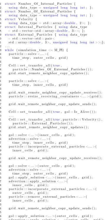
1 s t r u c t Number_Of_Internal_Particles {
2 u s i n g data_type = u n s i g n e d l o n g l o n g i n t; } ; 3 s t r u c t Number_Of_External_Particles {
4 u s i n g data_type = u n s i g n e d l o n g l o n g i n t; } ; 5 s t r u c t V e l o c i t y {
6 u s i n g data_type = s t d : : array <double, 2>; } ; 7 s t r u c t I n t e r n a l _ P a r t i c l e s { u s i n g data_type 8 = s t d : : v e c t o r <s t d : : array <double, 3>>; } ; 9 s t r u c t E x t e r n a l _ P a r t i c l e s { u s i n g data_type 10 = s t d : : v e c t o r <s t d : : p a i r <
11 s t d : : array <double, 3>, u n s i g n e d l o n g l o n g i n t> >;}; 12 . . .
13 w h i l e ( s i m u l a t i o n _ t i m e <= M_PI) { 14 p a r t i c l e : : s o l v e < . . . > (
15 time_step , o u t e r _ c e l l s , g r i d ) 16
17 C e l l : : s e t _ t r a n s f e r _ a l l (t r u e,
18 p a r t i c l e : : Number_Of_External_Particles ( ) ) ; 19 g r i d . start_remote_neighbor_copy_updates ( ) ; 20
21 p a r t i c l e : : s o l v e < . . . > (
22 time_step , i n n e r _ c e l l s , g r i d ) 23
24 g r i d . wait_remote_neighbor_copy_update_receives ( ) ; 25 p a r t i c l e : : r e s i z e _ r e c e i v i n g _ c o n t a i n e r s < . . . > ( g r i d ) ; 26
27 g r i d . wait_remote_neighbor_copy_update_sends ( ) ; 28
29 C e l l : : s e t _ t r a n s f e r _ a l l (t r u e, g o l : : I s _ A l i v e ( ) ) ; 30 . . .
31 C e l l : : s e t _ t r a n s f e r _ a l l (t r u e, p a r t i c l e : : V e l o c i t y ( ) , 32 p a r t i c l e : : E x t e r n a l _ P a r t i c l e s ( ) ) ;
33 g r i d . start_remote_neighbor_copy_updates ( ) ; 34
35 g o l : : s o l v e < . . . > ( i n n e r _ c e l l s , g r i d ) ; 36 a d v e c t i o n : : s o l v e < . . . > (
37 time_step , i n n e r _ c e l l s , g r i d )
38 p a r t i c l e : : i n c o r p o r a t e _ e x t e r n a l _ p a r t i c l e s < . . . > ( 39 i n n e r _ c e l l s , g r i d ) ;
40
41 g r i d . wait_remote_neighbor_copy_update_receives ( ) ; 42
43 g o l : : s o l v e < . . . > ( o u t e r _ c e l l s , g r i d ) ; 44 a d v e c t i o n : : s o l v e < . . . > (
45 time_step , o u t e r _ c e l l s , g r i d )
46 g o l : : a p p l y _ s o l u t i o n < . . . > ( i n n e r _ c e l l s , g r i d ) ; 47 a d v e c t i o n : : a p p l y _ s o l u t i o n < . . . > (
48 i n n e r _ c e l l s , g r i d ) ;
49 p a r t i c l e : : i n c o r p o r a t e _ e x t e r n a l _ p a r t i c l e s < . . . > ( 50 o u t e r _ c e l l s , g r i d ) ;
51 p a r t i c l e : : r e m o v e _ e x t e r n a l _ p a r t i c l e s < . . . > ( 52 i n n e r _ c e l l s , g r i d ) ;
53
54 g r i d . wait_remote_neighbor_copy_update_sends ( ) ; 55
56 g o l : : a p p l y _ s o l u t i o n < . . . > ( o u t e r _ c e l l s , g r i d ) ; 57 a d v e c t i o n : : a p p l y _ s o l u t i o n < . . . > ( o u t e r _ c e l l s , g r i d ) ; 58 p a r t i c l e : : r e m o v e _ e x t e r n a l _ p a r t i c l e s < . . . > (
59 o u t e r _ c e l l s , g r i d ) ; 60
61 s i m u l a t i o n _ t i m e += time_step ; 62 }
Listing 6.Illustration of the time stepping loop of a parallel pro-gram playing Conway’s Game of Life, solving the advection equa-tion and propagating particles in an external velocity field. Code from parallel advection simulation (Listing 5) did not have to be changed. Variables of the particle propagation model are also shown.
Table 1.Summary of application programming interface of generic simulation cell class. Listed functions are members of the cell class unless noted otherwise.
Code Explanation Usage example on line # of Listing 2
template<class TP, class... Variables>
Transfer policy and arbitrary number of variables to be stored in a cell type given as template arguments
9
operator[] (const Vari-able& v)
Returns a reference to given variable’s data
22
get_mpi_datatype() Returns MPI trans-fer information for variables selected for transfer
28
set_transfer(const bool b, const Variables&. . . vs)
Switches on or off transfer of given vari-ables in a cell
not used
set_transfer_all(const boost::tribool b, const Variables&. . . vs)
Static class function for switching the transfer of given variables in all cell instances on, off or to be decided on a cell-by-cell basis by set_transfer()
25
Member operators + =, − =, ∗ =, /= and free operators+, −,∗and /
Operations for two cells of the same type or a cell and standard types, the operator is applied to each variable stored in given cell(s)
not used
where the variables are used. This can potentially be eas-ily accomplished, for example, by wrapping the type of each variable in the boost::optional2type.
5 Coupling models that use generic simulation
cell method
In the combined model shown in the previous section, the submodels cannot affect each other as they all use different variables and are thus unable to modify each other’s data. In order to couple any two or more submodels new code must be written or existing code must be modified. The complexity of this task depends solely on the nature of the coupling. In simple cases where the variables used by one solver are only
2http://www.boost.org/doc/libs/1_57_0/libs/optional/doc/html/
1 i f ( s t d : : fmod ( s i m u l a t i o n _ t i m e , 1 ) < 0 . 5 ) {
2 p a r t i c l e : : s o l v e <
3 C e l l ,
4 p a r t i c l e : : Number_Of_Internal_Particles ,
5 p a r t i c l e : : Number_Of_External_Particles , 6 a d v e c t i o n : : V e l o c i t y , // c l o c k−w i s e
7 p a r t i c l e : : I n t e r n a l _ P a r t i c l e s ,
8 p a r t i c l e : : E x t e r n a l _ P a r t i c l e s 9 >(time_step , o u t e r _ c e l l s , g r i d )
10 } e l s e {
11 p a r t i c l e : : s o l v e <
12 C e l l ,
13 p a r t i c l e : : Number_Of_Internal_Particles , 14 p a r t i c l e : : Number_Of_External_Particles ,
15 p a r t i c l e : : V e l o c i t y , // c o u n t e r c l o c k−w i s e
16 p a r t i c l e : : I n t e r n a l _ P a r t i c l e s ,
17 p a r t i c l e : : E x t e r n a l _ P a r t i c l e s
18 >(time_step , o u t e r _ c e l l s , g r i d ) 19 }
Listing 7.Example of one way coupling between the parallel ad-vection and particle propagation models. The clock-wise rotating velocity field of the advection model (line 6) is periodically used by the particle propagation model instead of the counter clock-wise rotating velocity field of the particle propagation model (line 15).
switched to variables of another solver, only the template pa-rameters given to the solver have to be switched.
Listing 7 shows an example of a one way coupling of the parallel particle propagation model with the advection model by periodically using the velocity field of the ad-vection model in the particle propagation model. A similar approach could be relevant, e.g., in modeling atmospheric transport of volcanic ash in velocity fields of a weather pre-diction model (Kerminen et al., 2011). On line 6 the parti-cle solver is called with the velocity field of the advection model, while on line 15 the particle model’s regular veloc-ity field is used. More complex cases of coupling, which re-quire, e.g., additional variables or transferring variable data between processes, are also simple to accomplish from the software development point of view. Additional variables can be freely inserted into the generic cell class and used by new couplers without affecting other submodels and the transfer of new variables can be activated by inserting calls to, e.g., the generic cell’s set_transfer_all() function as needed.
6 Effect on serial and parallel performance
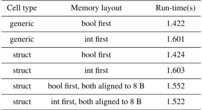
In order to be usable in practice, the generic cell class should not slow down a computational model too much and ide-ally neither serial nor parallel performance should be af-fected when compared to hand-written code with identical functionality. I test this using two programs: a serial GoL model and a parallel particle propagation model. The tests are conducted on a four core 2.6 GHz Intel Core i7 CPU with 256 kB L2 cache per core, 16 GB of 1600 MHz DDR3 RAM and the following software: OS X 10.9.2, GCC 4.8.4_0 from
Table 2.Run-times of serial GoL programs using different cell types and memory layouts for their variables compiled with GCC 4.8.4.
Cell type Memory layout Run-time(s)
generic bool first 1.422
generic int first 1.601
struct bool first 1.424
struct int first 1.603
struct bool first, both aligned to 8 B 1.552
struct int first, both aligned to 8 B 1.522
MacPorts, Open MPI 1.8.4, Boost 1.56.0 and dccrg commit 7d5580a30 dated 12 January 2014 from the c++11 branch at https://gitorious.org/dccrg/dccrg. The programs are com-piled with –O3 –std=c++0x. Where available/supported the options –march=native and –mtune=native were found to increase program speed by about 0.2 % with GCC on an-other machine and 3 % with Clang on the hardware described above.
6.1 Serial performance
Serial performance of the generic cell is tested by play-ing GoL for 30 000 steps on a 100 by 100 grid with peri-odic boundaries and allocated at compile time. Performance is compared against an implementation using struct {
bool; int; }; as the cell type. Both implementations
6.2 Parallel performance
Parallel performance of the generic cell class is evaluated with a particle propagation test which uses more com-plex variable types than the GoL test in order to empha-size the computational cost of setting up MPI transfer in-formation in the generic cell class and a manually written reference cell class. Both implementations are available in the directory https://github.com/nasailja/gensimcell/tree/1.0/ tests/parallel/particle_propagation/. Parallel tests are com-piled with GCC and are run using three processes and the fi-nal time is the average of the times reported by each process. Similarly to the serial case, each test is executed five times, outliers are discarded and the final result averaged over the remaining three runs. The tests are run on a 203grid without
periodic boundaries and RANDOM load balancing is used to emphasize the cost of MPI transfers. The run-time of the generic cell class version is 2.2 s and the reference program is 3.1 s. The extra time in reference program is spent in MPI regions but more detailed profiling was not done as the point is only to show that the generic simulation cell class does not slow down the parallel program. The output files of the differ-ent versions are bit iddiffer-entical if the same number of processes is used. When using recursive coordinate bisection load bal-ancing, the run-times of both are about 0.5 s with the refer-ence program being 10 % slower. A similar result is expected for a larger number of processes as the bottleneck will likely be in the actual transfer of data instead of the logic for setting up the transfers.
7 Converting existing software
Existing software can be gradually converted to use a generic cell syntax but the details depend heavily on the modularity of said software and especially on the way data in transferred between processes. If a grid library decides what to transfer and where and the cells provide this information via an MPI data type, conversion will likely require only small changes. Listing 8 shows an example of converting a Conway’s GoL program using cell-based storage (after Listing 4 of Honko-nen et al., 2013) to the application programming interface used by the generic cell class. In this case the underlying grid library handles data transfers between processes so the only additions required are empty classes for denoting simulation variables and the corresponding [] operators for accessing the variables’ data. With these additions the program can be con-verted step-by-step to use the generic cell class API and once completed the cell implementation shown in Listing 8 can be swapped with the generic cell.
1 s t r u c t g a m e _ o f _ l i f e _ c e l l { 2 i n t data [ 2 ] ;
3
4 s t d : : t u p l e < 5 v o i d∗, 6 i n t,
7 MPI_Datatype
8 > get_mpi_datatype ( ) c o n s t { 9 r e t u r n s t d : : make_tuple ( 10 (v o i d∗) &(t h i s−>data [ 0 ] ) ,
11 1 ,
12 MPI_INT
13 ) ;
14 }
15 } ; 16
17 s t r u c t I s _ A l i v e { } ; 18 s t r u c t Live_Neighbors { } ; 19
20 s t r u c t game_of_life_cell_compat { 21 . . .
22 i n t& o p e r a t o r[ ] (c o n s t I s _ A l i v e &) { 23 r e t u r n t h i s−>data [ 0 ] ;
24 }
25
26 i n t& o p e r a t o r[ ] (c o n s t Live_Neighbors &) { 27 r e t u r n t h i s−>data [ 1 ] ;
28 }
29 } ;
Listing 8.An example of converting existing software to use an ap-plication programming interface (API) identical to the generic cell class. API conversion consists of adding empty classes for denoting simulation variables on lines 17 and 18, and adding [] operators for accessing the variables’ data on lines 22–28. Line 21 is identical to lines 2–14.
8 Discussion
The presented generic simulation cell method has several ad-vantages over implementations using less generic program-ming methods:
1. The changes required for combining and coupling mod-els that use the generic simulation cell class are minimal and in the presented examples no changes to existing code are required for combining models. This is advan-tageous for program development as submodels can be tested and verified independently and also subsequently used without modification which decreases the possibil-ity of bugs and increases confidence in the correct func-tioning of the larger program.
vari-ables of one model will be used directly by another one without the first model having to export the data to an in-termediate format. This again decreases the chance for bugs by reducing the required development effort and by allowing the compiler to perform type checking for the entire program and warn in cases of, e.g., undefined behavior (Wang et al., 2012).
3. Arguably code readability is also improved by making simulation variables separate classes and making mod-els a composition of such variables. Shorthand notation for accessing variables’ data is also possible if the re-duction in verbosity is deemed acceptable:
constexpr Mass_Density Rho{}; constexpr Velocity V{};
cell_data[Rho] = ...; cell_data[V][0] = ...; cell_data[V][1] = ...; ...
For many intents and purposes the presented cell class acts identically to the standard heterogeneous container std::tuple (see also Sect. 3 on using tuple as a substitute in serial code) while providing additional syntactical sugar for serial pro-grams and helpful functionality for distributed memory par-allel programs.
For example the question of memory layout of simulation variables, whether each simulation variable should be stored contiguously in memory or interleaved with other variables at the same location in the simulated volume, also applies not only to using standard C++ containers but also to other programming languages as well. The key factor in this case seems to be the locality principle (Denning, 2005), i.e., that all hierarchies of computer (registers, caches, etc.) storage are reused as efficiently as possible while processing. For simulations modeling systems of multiple coupled equations it could well be that storing related variables, representing the same location of the simulated volume, contiguously in memory leads to faster execution than storing each variable separately from others. This is because, e.g., the smallest unit a CPU cache operates on is of the order of 100 bytes3 so fetching variables of one neighbor cell can lead to many more reads from memory if each variable is stored in a sepa-rate array instead of being stored close to the neighbor’s other variables. It should be quite simple to add the functionality of the cell class presented here to an existing grid library that would store all variables in separate contiguous arrays but this might not result in faster program execution and would violate at least rules 5 and 33 of Sutter and Alexandrescu (2011), namely “give one entity one cohesive responsibility” and “prefer minimal classes to monolithic classes”. If such
3Cache Hierarchy in http://www.intel.com/
content/dam/www/public/us/en/documents/manuals/ 64-ia-32-architectures-optimization-manual.pdf
functionality is absolutely necessary one could store e.g., one DCCRG grid (which itself stores only one type such as dou-ble in each of its own cells) in each variadou-ble given to the generic simulation cell class.
Other methods of speeding up a program, such as vector-ization and threading, do not seem to be affected by using the generic simulation cell class. For example the run-time of a threaded version of the combined parallel program (available in https://github.com/nasailja/gensimcell/blob/1.0/examples/ combined/parallel_async.cpp), which uses std::async to (po-tentially) launch each solver in a new thread at each time step, is reduced to less than 75 % of the original program on the system described in Sect. 6.1 when using a 100 by 100 grid without I/O. As different solvers cannot access each other’s data they can be run simultaneously in different threads. If submodels are coupled (e.g., in Listing 7) standard concurrency mechanisms can be used such as std::atomic or std::mutex. Access to entire simulation cells can be serial-ized with a mutex or it can guard a group of related variables (e.g., one for each of lines 39 and 40 in Listing 1) or single variables.
The possibility of using a generic simulation cell approach in the traditional high-performance language of choice – Fortran – seems unlikely as it currently lacks support for compile-time generic programming (McCormack, 2005). For example, a recently presented computational fluid dy-namics package implemented in Fortran, using an object-oriented approach and following good software development practices (Zaghi, 2014), uses hard-coded names for variables throughout the application. Thus, if the names of any vari-ables had to be changed for some reason, e.g., coupling to another model using identical variable names, all code using those variables would have to be modified and tested to make sure no bugs have been introduced.
9 Conclusions
I present a generic simulation cell method which allows one to write generic and modular computational models without sacrificing serial or parallel performance or code readability. I show that by using this method it is possible to combine several computational models without modifying any exist-ing code and only write new code for couplexist-ing models. This is a significant advantage for model development which re-duces the probability of bugs and eases development, testing and validation of computational models. Performance tests indicate that the effect of the presented generic simulation cell class on serial performance is negligible and parallel per-formance may even improve noticeably when compared to hand-written MPI logic.
Acknowledgements. The author gratefully acknowledges Alex Glo-cer for insightful discussions and the NASA Postdoctoral Program for financial support.
Edited by: P. Jöckel
References
Denning, P. J.: The Locality Principle, Communications of the ACM, 48, 19–24, doi:10.1145/1070838.1070856, 2005. Du Toit, S.: Working Draft, Standard for Programming Language
C++, ISO/IEC, available at: http://www.open-std.org/jtc1/sc22/ wg21/docs/papers/2012/n3337.pdf (last access: 4 March 2015), 2012.
Eller, P., Singh, K., Sandu, A., Bowman, K., Henze, D. K., and Lee, M.: Implementation and evaluation of an array of chem-ical solvers in the Global Chemchem-ical Transport Model GEOS-Chem, Geosci. Model Dev., 2, 89–96, doi:10.5194/gmd-2-89-2009, 2009.
Gardner, M.: Mathematical Games, Sci. Am., 223, 120–123, doi:10.1038/scientificamerican1170-116, 1970.
Hill, C., DeLuca, C., Balaji, V., Suarez, M., and Silva, A. D.: The Architecture of the Earth System Modeling Framework, Comput. Sci. Eng., 6, 18–28, doi:10.1109/MCISE.2004.1255817, 2004. Honkonen, I., von Alfthan, S., Sandroos, A., Janhunen, P., and
Palmroth, M.: Parallel grid library for rapid and flexible simu-lation development, Comput. Phys. Commun., 184, 1297–1309, doi:10.1016/j.cpc.2012.12.017, 2013.
Jöckel, P., Sander, R., Kerkweg, A., Tost, H., and Lelieveld, J.: Tech-nical Note: The Modular Earth Submodel System (MESSy) – a new approach towards Earth System Modeling, Atmos. Chem. Phys., 5, 433–444, doi:10.5194/acp-5-433-2005, 2005.
Kerminen, V.-M., Niemi, J. V., Timonen, H., Aurela, M., Frey, A., Carbone, S., Saarikoski, S., Teinilä, K., Hakkarainen, J., Tammi-nen, J., Vira, J., Prank, M., Sofiev, M., and Hillamo, R.: Charac-terization of a volcanic ash episode in southern Finland caused by the Grimsvötn eruption in Iceland in May 2011, Atmos. Chem. Phys., 11, 12227–12239, doi:10.5194/acp-11-12227-2011, 2011. Larson, J., Jacob, R., and Ong, E.: The Model Coupling Toolkit: A New Fortran90 Toolkit for Building Multiphysics Paral-lel Coupled Models, Int. J. High Perform. C., 19, 277–292, doi:10.1177/1094342005056115, 2005.
McCormack, D.: Generic Programming in Fortran with Forpedo, SIGPLAN Fortran Forum, 24, 18–29, doi:10.1145/1080399.1080401, 2005.
Miller, G.: A Scientist’s Nightmare: Software Problem Leads to Five Retractions, Science, 314, 1856–1857, doi:10.1126/science.314.5807.1856, 2006.
Musser, D. R. and Stepanov, A. A.: Generic programming, in: Sym-bolic and Algebraic Computation, edited by: Gianni, P., Vol. 358 of Lecture Notes in Computer Science, 13–25, Springer Berlin Heidelberg, doi:10.1007/3-540-51084-2_2, 1989.
Oberkampf, W. L. and Trucano, T. G.: Verification and validation in computational fluid dynamics, Prog. Aerosp. Sci., 38, 209–272, doi:10.1016/S0376-0421(02)00005-2, 2002.
Post, D. E. and Votta, L. G.: Computational science demands a new paradigm, Physics Today, 58, 35–41, doi:10.1063/1.1881898, 2005.
Redler, R., Valcke, S., and Ritzdorf, H.: OASIS4 – a coupling soft-ware for next generation earth system modelling, Geosci. Model Dev., 3, 87–104, doi:10.5194/gmd-3-87-2010, 2010.
Stroustrup, B.: Learning Standard C++ As a New Language, C/C++ Users J., 17, 43–54, 1999.
Sutter, H. and Alexandrescu, A.: C++ Coding Standards, C++ In-Depth Series, Addison-Wesley, available at: http://www.gotw.ca/ publications/c++cs.htm (last access: 4 March 2015), 2011. Thomas, W. M., Delis, A., and Basili, V. R.: An Analysis of Errors
in a Reuse-oriented Development Environment, J. Syst. Softw., 38, 211–224, doi:10.1016/S0164-1212(96)00152-5, 1997. Toth, G., Sokolov, I. V., Gombosi, T. I., Chesney, D. R., Clauer,
C. R., De Zeeuw, D. L., Hansen, K. C., Kane, K. J., Manchester, W. B., Oehmke, R. C., Powell, K. G., Ridley, A. J., Roussev, I. I., Stout, Q. F., Volberg, O., Wolf, R. A., Sazykin, S., Chan, A., Yu, B., and Kota, J.: Space Weather Modeling Framework: A new tool for the space science community, J. Geophys. Res.-Space, 110, A12226, doi:10.1029/2005JA011126, 2005.
Veldhuizen, T. L. and Gannon, D.: Active Libraries: Rethinking the roles of compilers and libraries, in: In Proceedings of the SIAM Workshop on Object Oriented Methods for Inter-operable Scien-tific and Engineering Computing (OO-98, SIAM Press, 1998. Waligora, S., Bailey, J., and Stark, M.: Impact Of Ada And
Object-Oriented Design In The Flight Dynamics Division At Goddard Space Flight Center, Tech. rep., National Aeronautics and Space Administration, Goddard Space Flight Center, 1995.
Wang, X., Chen, H., Cheung, A., Jia, Z., Zeldovich, N., and Kaashoek, M. F.: Undefined Behavior: What Happened to My Code?, in: Proceedings of the Asia-Pacific Workshop on Systems, APSYS’12, 9:1–9:7, ACM, New York, NY, USA, doi:10.1145/2349896.2349905, 2012.
Zaghi, S.: OFF, Open source Finite volume Fluid dynamics code: A free, high-order solver based on parallel, modular, object-oriented Fortran API, Computer Physics Communications, 185, 2151–2194, doi:10.1016/j.cpc.2014.04.005, 2014.