FELIPE MACHINI MALACHIAS MARQUES
MODELING, SIMULATION AND CONTROL OF A GENERIC
TILTING ROTOR MULTI-COPTER
FEDERAL UNIVERSITY OF UBERLÂNDIA
SCHOOL OF MECHANICAL ENGINEERING
FELIPE MACHINI MALACHIAS MARQUES
MODELING, SIMULATION AND CONTROL OF A GENERIC TILTING ROTOR
MULTI-COPTER
Master Thesis presented to the
Mechanical Engineering Graduate
Program of the Federal University of Uberlândia, as a partial fulfillment of the requirements for the degree of MASTER IN MECHANICAL ENGINEERING
Focus Area: Solid Mechanics and Vibrations
Advisor: Prof. Dr. Leonardo Sanches Co-advisor: Prof. Dr. Roberto Mendes Finzi Neto
Dados Internacionais de Catalogação na Publicação (CIP) Sistema de Bibliotecas da UFU, MG, Brasil.
M357m 2018
Marques, Felipe Machini Malachias, 1992-
Modeling, simulation and control of a generic tilting rotor multi-copter / Felipe Machini Malachias Marques. - 2018.
112 f. : il.
Orientador: Leonardo Sanches.
Coorientador: Roberto Mendes Finzi Neto.
Dissertação (mestrado) - Universidade Federal de Uberlândia, Programa de Pós-Graduação em Engenharia Mecânica.
Disponível em: http://dx.doi.org/10.14393/ufu.di.2018.1135 Inclui bibliografia.
1. Engenharia mecânica - Teses. 2. Veículo aéreo não tripulado - Teses. 3. Rotor de inclinação - Teses. I. Sanches, Leonardo. II. Finzi Neto, Roberto Mendes. III. Universidade Federal de Uberlândia. Programa de Pós-Graduação em Engenharia Mecânica. IV. Título.
iii
iv
Acknowledgments
This work is a result of years of hard working which initiated as a pioneering research project from the Federal University of Uberlândia Aeronautical Engineering undergraduate course on unmanned aerial system. The project was conducted by Prof Dr Leonardo Sanches and Prof Dr Roberto Mendes Finzi Neto to whom I express my gratitude for the opportunity, confidence and support through the project development.
After three years from the project beginning a vision has become true when the Aeronautical Engineering course direction has given a reserved place to develop our researches and experiments which now developed to the Laboratório de Aeronaves Autônomas. I also thank all the people involved who made it possible. Further, I show my gratitude to my research lab colleagues Ivan Tarifa, Matheus Amarante, Bruno Luiz Pereira and Douglas Lopes Silva for the support and teamwork and my classmates Marcelo Samora for his friendship from so many years.
To the Federal University of Uberlândia and the School of Mechanical Engineering of the opportunity to take this course and the mission to guide me through the scientific path and human development.
To the Brazilian research agency CNPq (National Council for Scientifc and Technological Development) for the financial support.
v
Keywords: Unmanned Aerial Vehicle, multi-copter, tilt rotor, Linear Quadratic Regulator
MARQUES, F. M. M. Modeling, Simulation and Control of a Generic Til-rotor Multi-copter.
2018, 99p. Master Thesis, Federal University of Uberlândia, Uberlândia – MG, Brazil
Abstract
In general, standard multi-copters are classified as underactuated systems since their number of control inputs are insufficient to allow the control of position and orientation independently. In this context, this work deals with the dynamical modeling of a generic of a tilted rotor multi-copter aerial vehicle and the design of a trajectory tracking controller using modern control techniques. The dynamical model is developed using Newton-Euler equations of motion considering the aircraft as a six degrees of freedom rigid body and also assuming that each rotor is capable of two independent movements (tilt laterally and longitudinally) introducing more control inputs to the system.
Later, the equations of motion are linearized around the desired trimmed operating conditions, considering small perturbations, based on the mission application so that the linear modern control techniques can be applied. The control method applied is a Linear Quadratic Tracking (LQT) controller formulated as a servomechanism problem permitting the controller to be designed for different reference input signals based on their time differential equations. The dynamical model and control law were validated using Matlab/Simulink® environment assuming
all the deriving non-linear effects caused by tilt actuation using as research object a real quadcopter model developed by the Laboratório de Aeronaves Autônomas from the Federal University of Uberlândia.
vi
Palavras chave: Veículos Aéreos Não Tripulados, multirrotores, tilt rotor, Regulador Linear Quadrático
MARQUES, F. M. M. Modelagem Simulação e Controle de uma aeronave Multirrotora com
Configuração Tilt-rotor. 2018, 99p. Dissertação de Mestrado, Universidade Federal de Uberlândia, Uberlândia – MG, Brasil
Resumo
Em geral, aeronaves multirrotoras convencionais são classificadas como sistemas dinâmicos subatuados uma vez que seu número de variáveis de controle é insuficiente para permitir que posição e atitude sejam controladas de forma independente. Desta forma, este trabalho trata da modelagem dinâmica genérica de uma aeronave multirrotora com configuração tilt-rotor e a aplicação das técnicas de controle moderno de forma a viabilizar o sistema a seguir uma trajetória. A modelagem dinâmica é feita baseada nas equações do movimento de Newton-Euler considerando a aeronave como um corpo rígido com seis graus de liberdade e ainda assumindo que cada motor seja capaz de executar dois tipos de movimento independentes (lateralmente ou longitudinalmente) introduzindo mais sinais de controle ao sistema.
Em seguida, as equações do movimento são linearizadas utilizando a teoria de pequenas perturbações em tordo de uma posição de equilíbrio baseada na missão requerida de forma que as teorias de controle moderno possam ser aplicadas. A técnica de controle empregada é a Linear Quadratic Tracking (LQT) formulada como um problema de servomecanismo permitindo que o controlador seja projetado para diferentes sinais de entrada baseados em suas equações diferenciais. O modelo dinâmico e a lei de controle são validadas utilizando o ambiente do Matlab/Simulink®
considerando os efeitos não lineares causados pelo mecanismo de tilt rotor utilizando como objeto de estudo um modelo quadrirrotor real desenvolvido pelo Laboratório de Aeronaves Autônomas da Universidade Federal de Uberlândia.
List of symbols
A state matrix
cl
A closed loop state matrix
prop
A propeller blade section area
b propeller drag coefficient
BCS Body Coordinate System
B input matrix
C output state matrix
D
C propeller section drag coefficient
CG aircraft center of gravity
T
C aerodynamic thrust coefficient
Q
C aerodynamic torque coefficient
g gravity
ICS Inertial Coordinate System
m
J propeller moment of inertia w.r.t. its rotating axis
xx
J , Jyy, Jzz aircraft moments of inertia
xy
J , Jyz, Jzx aircraft products of inertia
k thrust factor
d
k aircraft drag coefficient
K torque constant
v
K voltage constant
t
K electrical torque constant
l multi-copter arm length
air
m air mass
MCS Motor Coordinate System
ix
air density
k
rotor weighting matrix
damping ratio
k
tilting mechanism weighting matrix
propeller angular speed
0
trimmed propeller angular speed
n
natural frequency
Summary
1. Introduction………..1
1.1Motivations and Objectives ... 1
1.2 Unmanned Aerial Vehicles (UAVs) ... 2
1.3 MAVs Classification ... 4
1.4 The Multi-rotors ... 7
1.4.1 Number of rotors ... 7
1.4.2 Actuation Mechanism ... 8
1.5 Control Techniques ... 10
2. System Modeling …...………12
2.1 Reference Frames and Kinematic Relations ... 12
2.2 Equations of Motion ... 16
2.3 External Forces ... 19
2.3.1 Thrust ... 19
2.3.2 Drag ... 22
2.3.3 Gravitational Force ... 23
2.4 External Moments ... 23
2.4.1 Thrust Vector Torque ... 23
2.4.2 Gyroscopic Effect ... 25
2.4.3 Fan Torque ……….26
2.5 Final Dynamical Model ... 27
2.6 Linearization ... 28
3. Modern Control ………31
xii
3.2 Linear Quadratic Regulator ... 33
3.2.1 Quadratic Performance Index ... 33
3.2.2 The Regulator Problem ... 35
3.3 Tracking a Command ... 37
4. Apparatus and Procedures …….………41 4.1 The Multi-rotor ... 41
4.1.1 Quadcopter Structure ... 42
4.1.2 Propulsion System ... 42
4.1.3 Microcontroller ... 43
4.1.4 The Tilting Mechanism ... 44
4.1.5 Inertial Measuring Unit ... 46
4.2 Numerical Simulations ... 46
5. Results and Discussions ...49
5.1 Checking Controllability and Observability ... 49
5.2 Step Input Position Signal ... 52
5.2.1 Choice of Weighting Matrices ... 52
5.2.2 Pole and Zeros Location Analysis ... 53
5.2.2 Time Response Analysis ... 57
5.3 Ramp Input Signal ... 68
5.3.1 Choice of Weighting Matrices ... 69
5.3.2 Poles and Zeros Analyses ... 69
5.3.3 Time Response Analysis ... 71
5.4 Sinusoidal Input Signal ... 74
5.4.1 Poles and Zeros Analysis ... 74
5.4.2 Time Domain Analysis ... 75
5.5 Random Space Trajectory ... 83
5.6 Conclusions and Highlights ... 88
xiii
6.1 Overview ... 90
6.2 Dynamical Model ... 90
6.3 Control Design ... 91
6.4 The Multi-copter ... 92
6.5 Simulations ... 92
6.6 Future Work ... 93
Chapter 1
Introduction
In this introductory chapter, first, the motivations and objectives which gave support to this work are outlined. Later, general information and definitions about unmanned aerial vehicles (UAVs) are presented highlighting their benefits for miniaturization. Further, a brief comparison of different types of aircraft configurations and applied control techniques, including the actuation mechanisms already developed in other works, are presented aiming the UAV control state of art.
1.1 Motivations and Objectives
The main aim and motivation of this present work is to investigate the dynamical behavior of a multi-rotor UAV considering a tilt-rotor actuation configuration. Later, a control law based on modern control theory is applied so that the aircraft is able to operate autonomously. Finally, the stability and efficiency of the closed loop system are analyzed aimed at different tilting mechanisms configurations and operational conditions.
On a practical point of view, the development of the project stands on the uprising UAV market share on the global scenario, and also on the upward demand for more efficient and versatile aircrafts for military and civilian applications. Based on current UAV applications, it can be observed that there is constant seek for aircrafts with better endurance, range, stability and capability to perform autonomous flights.
2
configuration is a possibility to solve the problem and also reduce the control energy of the spinning propellers so that the motors do not operate on saturation level (Cutler et al, 2011).
Regarding the control application, some recent works on tilting rotor UAVs proposed linear (Rajappa et al, 2015; Badr et al, 2016; Oosedo et al, 2015) and nonlinear (Ryll et al, 2012; Kendoul et al, 2006) control techniques for autonomous flight applications. However, there are also other control techniques which have shown good performance for fixed rotor multi-copters applications as compared on Bouabdallah (2007) and Suiçmez (2014) works.
Finally, the work yearns to contribute for the development of the recently created
Laboratório de Aeronaves Autônomas of Federal University of Uberlândia and the Aeronautical Engineering course. The laboratory aims to build its own multi-copter for multi tasks purposes. Most of commercially available platforms does not contemplate a detailed stability analysis based on the system response. Thus, checking the viability of the control law including a tilting-rotor mechanism through the design process can be crucial to increase the aircraft performance.
1.2 Unmanned Aerial Vehicles (UAVs)
In the last few years, unmanned aerial vehicles (UAVs) have made a great impact on aviation. As defined in Nonami et al (2013), an UAV is a powered aerial vehicle that does not carry an onboard crew, can operate with varying degrees of autonomy, and can be expendable and reusable. Usually, the vehicle is controlled remotely via a radio transmitter or an onboard control system. Considering safety and cost, UAVs are a turning point compared to manned air vehicles since it is not dependent of pilot. Thus, they can avoid risking human lives specially for dangerous situations such as, search and rescue, military operations, firefighting, etc; and also favors aircraft miniaturization.
3
a very versatile tool which could be applied on quotidian activities. Among the civilian applications for UAVs, some can be highlighted such as: aerial photography and filming, surveillance, remote sensing, crop analysis, data acquisition, etc. A survey from the BI Intelligence enterprise (Business Insider, 2016) has shown that the UAV worldwide market share will grow from 5 billion to 12 billion dollars on military applications while the civilian will be close to 4 billion dollars from 2013 to 2024 as presented on Fig. 1.1. Also, a major part of the investments is concentrated on Europe and the USA.
Figure 1.1 - UAV market share forecast. (Business Insider, 2016)
4
Table 1.1 - Common MAV requirements.
Specification Requirements
Size < 15 cm
Weight <100 g
Range 1 to 10 km
Endurance 60 min
Altitude < 150 m
Speed 15 m/s
Payload 20 g
Cost $ 1500.00
Notwithstanding, there are some properties which can be optimized on this aircraft category in order to make civilian applications even more feasible. Nowadays, academic researches are being developed in order to come up with MAV designs to fulfill the requirements of: endurance, range, maneuverability, low cost, better energy density (available energy/mass), autonomous flight capability, among others. Furthermore, governmental aviation agencies are working to develop a UAV specific legislation to guarantee the safety of the operations and monitor the applications. Hence, it is essential to assure that the new technologies are able to attend the legal requirements. Thus, quite a few control techniques for better stability has been investigated to increase aircraft performance under external disturbance, parameters uncertainty, presence of sensor noise. Further, researches on electronics aim to develop compact, lighter and more efficient electrical components.
Other works explore new actuation mechanisms that can be used to control the aircraft optimizing its flight properties. One of these mechanisms is the tilt-rotor configuration where the aircraft motor is attached to the aircraft in such manner that the thrust force vector generated by the propeller can be vectorized. This configuration has been recently investigated and has shown efficient results on multi-rotor MAVs and also on Vertical Take-off and Landing (VTOL) aircrafts and, for this reason, it will serve as motivation for this present work.
1.3 MAVs Classification
5
Figure 1.2 - Aircraft general classification. Adapted from: Bouabdallah (2007).
Even though each aircraft type has their own advantages and specific applications, just a few of them are feasible for miniaturization accounting the concept design of a MAV. Table 1.2 illustrates different state of art MAV projects highlighting their main advantages and disadvantages.
Further, according to Bouabdallah (2007), it is expected that compact, versatile and cheap MAV aircraft will correspond the major demand for UAV industry principally for quotidian civilian applications. Concerning this, the author proposes and picks out some different MAV configurations and quotes its characteristics on different aspects which should benefit the miniaturization as presented on Table 1.3. The analysis reveals that aircrafts with VTOL characteristics, including helicopters, tandem, coaxial, multi-rotors and blimps, have major advantages over the other configurations. These advantages are summarized on their hover, vertical and low speed flights, allowing them to operate in restricted space environments.
Concerning the helicopters, tandem and coaxial VTOL aircrafts, their speed, position and attitude control mechanism is based on variable pitch rotary wings, which has shown to be very mechanically complex. However, the multi-rotor VTOL configuration, in general, uses fixed pitch spinning propellers. On this case, the forces and moments control are based on the rotor angular speed variation (Suiçmez, 2014). For this reason, the multi-rotors take advantage over the other VTOL configurations due to their mechanical simplicity and also their lesser susceptibility to gyroscopic effects.
6
Table 1.2 - Common MAV configurations. Adapted from: Bouabdallah (2007).
Configuration Advantages Disadvantages Picture
Fixed Wing
(Trimble UX5) Simple mechanics, higher range and endurance Cannot perform hovering flight
Trimble (2017)
Helicopter (Scout B1-100)
Controllability,
memorability Complex mechanics, large rotor, tail rotor necessity
Aeroscout (2017)
Coaxial (Modlab) Compact geometry Complex aerodynamics
Paulos e Yim (2013)
Tandem (Dragonfly
DP-6) Simple aerodynamics, good controllability Size
Aeroscout (2017)
Multi-rotor (OS4) mechanics, higher payload Maneuverability, simple
capacity High energy consumption
Bouabdallah (2007)
Blimp (VAIRDO Brainbox)
Low energy consumption, higher range and
endurance
Size, maneuverability, low operational speed
Vairdo (2018)
Bird-like (Techject
Dragonfly) Compact geometry, good maneuverability
Complex mechanics / control, high energy
consumption Techject (2018)
Hybrid VTOL (University of
Calgary)
Hover flight, higher
endurance and range Complex mechanics
7
Table 1.3 - Flight principle comparison (1=bad, 3=good). Adapted from: Bouabdallah (2007).
Plane Helicopter Bird-Like Auto-giro Blimp
Energy cost 2 1 2 2 3
Control cost 2 1 1 2 3
Payload/volume 3 2 2 2 1
Maneuverability 2 3 3 2 1
Hover flight 1 3 2 1 3
Low speed flights 1 3 2 2 3
Vulnerability 2 2 3 2 2
VTOL 1 3 2 1 3
Endurance 2 1 2 1 3
Miniaturization 2 3 3 2 1
Indoor operations 1 3 2 1 2
Total 19 25 24 18 25
1.4 The Multi-rotors
Since the multi-rotors has shown to be a valuable candidate for many UAV applications, researchers and the industry developers have already tested many different configurations design based on missions’ specifications. Thus, this aircraft category can also be classified concerning the
number of rotors and the actuation mechanisms.
1.4.1 Number of rotors
8
Figure 1.3- Multi-rotors classification by the number of rotors. Sources (from left to right): FPV (2018), Thielicke (2017), Introbotics (2013) and Direct Industry (2018).
1.4.2 Actuation Mechanism
In general, in most part of the designed multi-rotor aircrafts, the position and attitude control are based on the rotor capacity to change its rotational speed independently. On this case, the propulsion group is attached to the aircraft structure and their propeller blades have fixed pitch angle. Some research application examples can be found on Bouabdaallah (2007), Fogelberg (2013) and Suiçmez (2014) as illustrated on Fig 1.4. Basically, the coordinated rotors angular speed variation generates forces and moments imbalance permitting the aircraft to control attitude and position.
9
However, as discussed in Badr et al. (2016), attitude and position cannot be controlled independently when using this actuation mechanism. Badr et al. (2016) presents this problem as under actuation, i.e. the number of input commands on the system is lower than the number of states to be controlled. Further, on this situation, the aircraft is only capable to perform a hover flight when the roll and pitch angles are zero, meaning that the aircraft is holding a horizontal position w.r.t the inertial coordinate frame.
On this manner, researchers have proposed some strategies in order to optimize multi-rotor control actuation. One of them is the tilt-rotor mechanism which consists on the rotor rotation w.r.t to the multi-rotor arm in a fashion that the thrust vector force produced by the spinning propeller can be vectorized. For instance, Rajappa et al (2015) designed a hexa-copter structure that efficiently explores the input signals since the rotors are can rotate freely around six parallel axes, dismissing the installation of extra actuators. Then, the tilt angles are optimized for each specific mission once the user give a planned trajectory.
Ryll et al (2012) developed a system where all the rotors are capable of rotating about the fixed arm longitudinal axis and their movement are performed by actuators attached to the extremity of multi-copter arm. Similarly, Hintz et al (2014) proposed a quadcopter composed by 8 rotors installed coaxially. Each pair of 4 rotors are connected by a rotating arm in such manner that they can move w.r.t to the central body using only one actuator. This configuration permits 90 degrees hovering flights w.r.t the inertial coordinate frame thus the aircraft is able to cross straight paths.
Finally, Giribet et al (2016) and Badr et al (2016) designed a tilt configuration which the rotors are capable of tilting about an axis normal to the rotors arm. This configuration uses one extra actuator for each multi-copter arm.
Some useful conclusions can be extracted from the research works about the tilt rotors which are:
• energy consumption reduction;
• position and attitude can be controlled independently;
• better maneuverability performance;
• the controller is able to reject external perturbations and keep flight even with a rotor failure.
10
since the system has a faster response compared to the fixed propeller system, the electric rotors are less susceptible to saturation on aggressive maneuvers. Finally, the aircraft is able to perform inverted flights once the propeller pitch angle is inverted. All the presented actuation mechanisms concepts are illustrated on Table 1.4.
Table 1.4 - Multi-rotor actuator mechanisms.
Mechanism Image
Longitudinal tilting mechanism
Badr et al (2015)
Lateral tilting mechanism
Ryll et al (2012)
No additional hardware
Rajappa et al (2015)
Variable pitch propeller mechanism
Cutler et al (2011)
1.5 Control Techniques
Independently of the actuation mechanism or structural design, the multi-copter system is considered as an open-loop unstable system. Hence, it is indispensable to insert a control technique so that it can operate, either autonomously or remotely, on safe conditions. Several control strategies have already been explored and compared either to guarantee the system stability (regulators) or for autonomous flights operations (trackers).
11
linearized around an operating point (trimming conditions) so that the linear control techniques can be applied. Among the commonly used linear control techniques, the most well-known are the Proportional Integral Derivative (PID), which is a Single Input Single Output (SISO) control technique, and the Linear Quadratic Regulator (LQR) that concerns a multi-state controller. In Bouabdallah (2004), both control techniques are compared while used on the stabilization of a quad-copter attitude test-bench with 3 degrees o freedom. The same techniques are employed for trajectory tracking on Raffo et al (2008), where numerical simulations are validated via experimental results.
For autonomous flights applications, linear control techniques present some limitations once the dynamical model linearization and simplification omits some non-linear dynamical effects which can significantly affect the system behavior (Kendou et al, 2007). Furthermore, there are uncertainty parameter problems, actuators saturation, noise and external disturbances that affects the plant and can bring the system to instability condition.
Additionally, since the non-linear control techniques are based on the stability condition of the non-linear model, they can present better robustness compared to the linear. The most common are: the Backstepping, H, Feedback Linearization and Sliding Mode Control. On his work, Rich
(2012) proposed a H controller to stabilize the rotation movements and a Backstepping controller
to control minimizes the difference between the aircraft current and desired positions, so that it can track a pre-defined trajectory.
Even though some control techniques being able to accomplish a specific task, it is also possible to distinguish them on some features as: energy consumption, steady state error, response time, actuator saturation and disturbance rejection. For instance, on his work, Suiçmez (2014) compared linear and non-linear control techniques such as LQR, LQT and Backstepping with the purpose of evaluate their operational parameters so that the multi-copter could operate autonomously with better efficiency.
In summary, each control techniques have its own advantages and drawbacks. For instance, on his work, Suiçmez (2014) has shown that the LQT controller may present less energy consumption and better disturbance rejection over the LQR and Backstepping controller. Further, on Bouabdallah (2007) PID, LQ, Sliding Mode and Backstepping controllers were compared and, it can be inferred that a combination of PID and Backstepping (also known as Integral Backsetpping) is the best control approach for multi-copter autonomous flight.
Chapter 2
System Modeling
The concept of this section is to derive the dynamical model of a generic multi-copter with
n rotors such that each rotor is capable of tilting in two different directions: laterally and
longitudinally with respect to the rotor’s arm, introducing more control inputs to the system. First, the reference frames used to develop the equations among with their kinematic relations will be presented in section 2.1. Then, the equations of motion of a general aircraft (fixed wing or multi-copter) will be developed in Section 2.1. On sequence, the external forces and moments acting on the multi-rotor body will be explained in section 2.3. Lastly, Section 2.4 contains the full non-linear dynamical model of the aircraft, and the equations are linearized around the trimming operating conditions based on mission applications in order to allow the linear control techniques to be applied.
Some considerations must be taken before the model development which are: - The aircraft structure is supposed rigid.
- The propellers are rigid.
- Earth’s gravitational field (g), mass of the quadrotor and body inertia matrix of the quadrotor (J) are constants.
- Thrust factor (k), torque factor (b) and the drag coefficient (kd) are constants.
- Inertia of the rotors are neglected.
2.1 Reference Frames and Kinematic Relations
21 3 2 2 2 w p T P R
(2.3.4)
Regarding the aerodynamic behavior of the propeller blade, from the momentum blade theory (Magnusson, 2014), it is possible to write the thrust force and torque generated by the spinning propeller which are presented, respectively, as:
4 2
p T R
T C (2.3.5)
5 2
p Q R C
(2.3.6)
where CT and CQ are aerodynamic constants for thrust and torque, respectively, which depends
on the blade section.
Moreover, considering that the produced torque is proportional to the thrust force by a constant K :
Q p T C K C R
(2.3.7)
Now, bearing in mind the electrical behavior of the motor, the torque ( ) produced by a brushless motor is proportional, by a constant (Kt), to the motor`s input current (i). However, it must be accounted a residual current (i0) corresponding to the current when there is no load in the
motor. Thus,
t o K i i
(2.3.8)
Further, the voltage (V ) applied to the motor considering the resistive loss, is given by:
Ω
m v
V iR K (2.3.9)
m
R and Kv being the motor electrical resistance and a proportional constant between the applied
voltage and the motor’s shaft angular speed.
Hence, the motor’s electrical power is obtained from Eqs. (2.3.8) and (2.3.9):
Ω
²
t o t o m m t v w
t
Ki K Ri R K K P iV
K
(2.3.10)
22
there is no load and is, consequently, small. Finally, the motor electrical power can be stated as follows:
~ v τΩ
w t
K P
K (2.3.11)
Thus, assuming that all the driver shaft is transferred to the propeller, Eq. (2.3.10) can substitute on Eq. (2.3.4) and isolating the thrust (T) gives:
2 2
2
2
v m Ω Ω
t
K K R
T k K
(2.3.12)
In conclusion, the thrust force produced by each rotor is proportional to the square of the angular speed of the rotor propeller by a constant k. So, the thrust vector generated by the n
motor-propulsive group, written on the MCS, is:
1 2 0 0 Ω n i i i MCS T T k
(2.3.13)The thrust vector can be oriented on the BCS applying the rotational matrix transformation from Eq. (2.1.10) on Eq, (2.3.13). Hence,
2 1 2 1 2 1sin( )sin( ) cos( )sin( )cos( )
cos( )sin( ) sin( )sin( )cos( )
cos( )cos( )
n
i i i i i i
i n
BCS i i i i i i
i
n
i i i i T k k k
(2.3.14) 2.3.2 DragIn this model, the drag due to the incoming viscous flow will be considered. For small multi-rotor applications, the viscous drag can be considered as proportional, by a constant kd, to the
30
1 1 1 1
1 1 1 1
1 1 1 1
1 1 1 1
1 2 2 0 0 2 2 0 0 0 2 2 0 0 0 2 2 0 0 0 0 sin cos 0 cos sin 0
2 0 0
bsin bcos 2 sin bcos bsin 2 cos (sin 2
t it t it
t it t it
i
t i t i
i t t
t i t i
i t t
t t i i i i i i i i i
xx xx xx
i i
i i
yy yy xx
i i zz
k k k k
m m
k k k k
m m
k
l k
J J J
l k
B J J J
l b J
1 1 1 1
2 0
cos )
0
0 0 0
0 0 0
0 0 0
0 0 0
0 0 0
0 0 0
t t it
i i zz l k J (2.6.7)
Chapter 3
Modern Control
Modern Control Theory has shown to be a valuable tool in aerospace industries for aircraft dynamic stabilization or autonomous flight operations. This control technique has efficiently been applied on commercial and military aircrafts, for instance, the Boeing 767 and the F-16 (Stevens and Lewis, 1992). Also, for MAVs application, the technique has revealed to be a valuable tool in the development of autonomous systems (Suiçmez, 2014).
Differently from fixed wing aircrafts, the multi-rotors are open-loop unstable and, therefore, must have a control loop integrated in order to make the flight possible. As presented in the previous chapter, the multi-rotor dynamics are represented as a MIMO system containing a large number of states and inputs. Therefore, the application of classic control techniques as PID control are unfeasible, since the controller is based on successively SISO transfer function closed loops. In this case, each loop gain should be selected individually by the designer using trial and error methods or optimization algorithms so that the design procedure becomes difficult.
According to Stevens and Lewis (1992), there are two central concepts to modern control system design. The first is that the design is based directly on the state-variable model introduced by Kalman (1960) (Eqs. (2.6.2) and (2.6.3)) and, just as stated by the authors, contains more information about the system than the input-output description.
The second central concept is the expression of performance specifications in terms of a mathematically precise criterion which then yields matrix equations for the control gains. These matrix equations are solved using computer algorithms so that all the loop control gains are computed simultaneously, guaranteeing the closed loop stability. In this case, the fundamental engineering decision is the selection of the suitable performance criterion based on the system response.
40
42
4.1.1 Quadcopter Structure
The preliminary concept design was proposed by Costa (2016) where the mechanical optimization of the arms was explored. The platform was designed with aid of a CAD software and manufactured using Printed Circuit Boards (PCB) and ABS such that, most of the components, could be built using a 3D printer. As a result, the structure is 624 mm in span and about 135 mm in height as illustrated in Fig 4.2.
Regarding the physical properties, the quadcopter mass was measured using a scale while the inertia properties was estimated from the CAD model. The aircraft mechanical properties are summarized in Table 4.1.
Figure 4.2 Quadcopter side view.
Table 4.1 Quadcopter parameters.
Property Parameter Value Unit [SI]
Number of rotors n 4 -
Mass m 0.620 kg
Inertia on xb axis Jxx 0.007 kg.m2
Inertia on yb axis Jyy 0.007 kg.m2
Inertia on zb axis Jzz 0.013 kg.m2
Drag coefficient kd 4.8e-3 N.s2
Arm length l 0.180 m
4.1.2 Propulsion System
43
angular speed) were obtained experimentally using a test bench as presented in Appendix A. Table 4.2 shows the E300 mechanical and operational properties.
The ESCs are connected to a power source (for external mission operations a 3S or 4S LiPo battery) and to a PWM output from the microcontroller.
Table 2 DJI® E300 properties.
Property Parameter Value Unit [SI]
Recommended load Tnom 300 g/axis
Maximum thrust Tmax 600 g/axis
Current im 15 A
Voltage Vm 11.1~14.8 V
Thrust coefficient k 8.901e-6 Ns2
Propeller moment of
inertia Jm 4.025e-5 kg.m2
Propeller drag
coefficient b 1.1e-6 Nms2
Arm length l 0.180 m
4.1.3 Microcontroller
44
Figure 4.3 BeagleBone Green microcontroller board (Brown, 2015).
4.1.4 The Tilting Mechanism
The quadcopter arm developed in Costa (2016) did not contemplate the tilting capability of the rotors. Hence, a tilting mechanism was designed so that the rotors are able to tilt longitudinally (rotation about ym axis) with the aid of an actuator. The choice of this configuration mechanism was essentially based on construction facility once the multi-copter arm has already been manufactured. The mechanism was printed on ABS using a 3D printer and weights approximately 12 g. The mounting mechanism dimensions are presented in Fig. 4.4 and it can be attached to the quadcopter arm at the rotating point OT. The rotor arm distance to the quadcopter CG was preserved.
So, the motor set (DC motor and propeller) is attached to the motor support (see Fig. 4.4) so that, when the actuator rotates, the connection rod rotates the motor bed around point OT ,
45
Figure 4.4 The tilting mechanism and its dimensions in mm.
The tilting mechanism is driven by a Hitech® HS-65MG actuator that is connected to the
motor bed by a rigid rod as illustrated in Fig. 4.5 permitting the bed rotation from 25 deg (left) to -50 deg (right). Also, the actuator is connected to the PWM microcontroller output so that its position can be set varying the signal pulse-width. The actuator specifications are presented in Table 4.3.
Table 4.3 HS-65MG actuator specifications.
At 4.8V At 6V
Speed 0.14s/60º 0.11s/60º
Torque 1.8 kg.cm 2.2 kg.cm
Weight 12.5 g
Dimension 23.6 x 11.6 x 24 mm
48
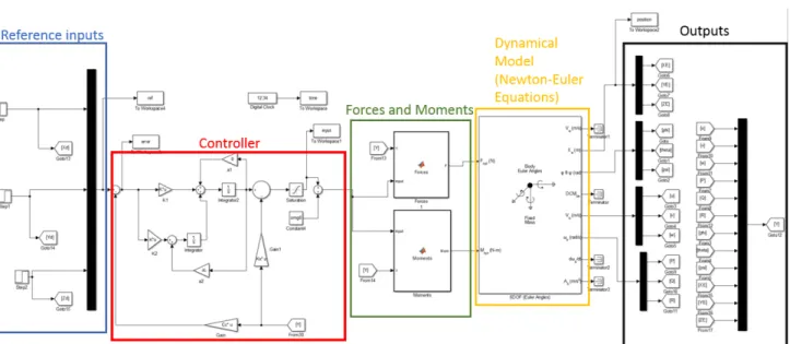
Figure 4.7 Matlab/Simulink block diagram.
In conclusion, the designed Matlab® routine permits control law gain matrices to be
calculated offline for different configurations while the Simulink model enables the numerical simulation using a nonlinear model. Therefore, some physical effects that were not previewed on the linearized model will affect the controller behavior, such as the gyroscopic effect and coupled variables. Further, the numerical analysis will be closer to the real problem and the controller robustness to perturbations can be observed. However, it must be stated that, due to the non-linearity level of the plant, the simulations may be susceptible to integration or numerical errors.
Chapter 5
Results and Discussions
In this chapter, the control technique presented on Chapter 3 will be tested by numerical simulations and the obtained results analyzed. The main goal of the analysis is to evaluate the stability and performance of the controller for different tilt-rotor configurations (no tilt mechanism, tilting laterally and tilting longitudinally) and subjected to diverse reference trajectories.
The object of study is the quad-copter aircraft described on Chapter 4 containing all physical parameters.
5.1 Checking Controllability and Observability
As discussed on Chapter 3 the controllability and observability conditions of a given system must be satisfied, otherwise the control cannot stabilize the system and perform as desired. Thus, the conditions of controllability and observability were checked for three different scenarios: no tilt mechanism, 4 and 2 tilting mechanisms laterally (
) and 4 and 2 tilting mechanisms longitudinally (). It is important to state that the position of the tilting mechanism affects the system dynamics and, for the cases with only 2 tilting mechanisms, they were positioned on two arms 90 deg to each other.The state-space system matrices (A and B) are obtained substituting the aircraft parameters from Chapter 4 on Eqs. (2.6.6) and (2.6.7) and it is considered that all the states can be measured so matrix C is I12 12x . Later, the controllability matrix is derived from Eq. (3.1.1). Once again, for a system with ns states, the system is controllable and observable if the matrices U and
b
O contains ns linearly independents columns or rows, in other words, U and Ob have full rank
s
n . On this case, ns 12 assuming the state vector from Eq. (2.6.4). The rank of matrices U and
b
50
It can be inferred from Table 5.1 that the system without and with longitudinal tilting mechanism does not accomplish the controllability conditions even though the observability is guaranteed. This implies that the system is not bounded and its response can diverge over time. On the other hand, the controller with lateral tilt mechanism has full rank for both 2 cases, so the system is called controllable.
Table 5.1 - Controllability and Observability conditions.
Configuration Rank Ob Rank U
No tilt 12 11
2 laterally (
) 12 124 laterally (
) 12 122 longitudinally () 12 11
4 longitudinally () 12 11
Analyzing only the controllability conditions, it is not possible to identify which of the states is not being controlled. However, looking at the linearized dynamical model, it can be observed that the yaw movement dynamics, including its respective angular rate, is dynamically independent from the other states. This fact can be verified looking at line 6 matrix A from Eq. (2.6.6) which is completed only by zeros.
Hence, the uncontrollability problem can be related with the yaw actuation mechanism. When the system has no tilt mechanism, the yaw torque is relied on the propeller drag coefficient (b parameter), which is very low. However, when the lateral tilt mechanism is added to on the multi-copter, the system becomes controllable since the yaw response due to the tilt angle variation is much more effective compared to the propeller drag response as observed on Fig. 5.1.
51
Thus, as shown on Table 5.2, the controllability and observability conditions are satisfied for the three cases when the yaw dynamics are not included in the model. Nevertheless, if the system does not have a yaw control, its response will become unstable since the aircraft will be able to spin around itself freely. Hence, to solve this problem, a separate controller can be designed separately just to guarantee that the yaw movement is stable. This design will be discussed lately.
Table 5.2 - Controllability and Observability conditions without considering yaw dynamics.
Configuration Rank Ob Rank U
No tilt 10 10
2 longitudinally () 10 10
4 longitudinally () 10 10
54
3
1 2
1 2 3
( ) t t t .... nt
n
x t C e C e C e C e (5.2.9)
being C C C1, ...2 n and 1, ...2 n complex constant values.
Regarding the values of , the exponentials from Eq. (5.2.9) assumes solutions that are oscillatory and/or decaying exponentially amplitudes. Also, assuming that the frequency of the damped oscillations can be written as:
1 2
j nj j i j
(5.2.10)
where n j and j are the natural frequencies and the damping ratios of i-th mode (eigenvector
related to each eigenvalue).
On the cases where
0, the system is considered undamped and a harmonic response is expected. If is complex and 0
1, the solutions are a decaying exponential combined with an oscillatory and the system is considered underdamped. Finally, when is pure real (
1), the solutions are simply a decaying exponential with no oscillation and the system is referred to as overdamped.First, checking the open-loop poles of the linearized system, i.e. the eigenvalues of A
matrix, it has 3 poles at 0.006 while the other are at 0 even if the yaw dynamics is included. Hence, the system has a decaying oscillatory response for some modes ( 0.006), which may be related to the linear velocity due to drag effect, and a steady response for others (
0
).
Moreover, Fig. 5.2 show the pole mapping for the closed loop system considering 5 different actuation mechanisms: no tilt mechanism, 2 and 4 longitudinal tilting mechanisms () and 2 and 4 lateral tilting mechanisms (
). It is important to note that the tilt mechanism is added to the system and works together with the spinning rotors. The poles closer to the origin are presented on Fig. 5.3.It can be concluded, from Figs. 5.2 and 5.3, that all the closed-loop poles (eigenvalues) are on the left half plane of the Real/Imaginary axis assuming real negative values. Thus, the solution is a decaying exponential (oscillatory or not) so the system converges to a finite value, i.e. the system is considered as asymptotically stable.
55
figures. Adding the tilting mechanism to the system brought the poles visible on Fig. 5.2 further from the imaginary axis compared to the open-loop poles, meaning that the pole natural frequency and/or the damping ratio has increased. Thus, the system is able to respond faster and/or more smoothly.
Figure 5.2 - Closed-loop poles for a first order integrator controller (step input signal) for five actuator configurations: no tilt, 4 lateral tilt, 2 lateral tilt, 4 longitudinal tilt and 2 longitudinal tilt.
56
Further, regarding Fig. 5.3, the poles tends to shift radially, meaning that the damping ratio is maintained while the natural frequency is increased, on this case the system will respond faster. This phenomenon is more effective when the lateral tilting mechanism is added the system and also when the number of tilting mechanisms is increased.
The zeros, or the numerator’s roots of each transfer function of the closed-loop system, can also play a major role on its response. According to Hoagg and Bernstein (2007), having an open-right-plane zero, an input signal can be unbounded, a phenomenon known as non-minimum-phase zero, directly affecting the steady state system’s response.
The zero mapping is presented on Figs. 5.4 and 5.5 for all system transfer functions five different scenarios as stated previously. One observes from the figures that the zero distribution does not follow a specific pattern. However, on Fig. 5.5, it can be seen that there are some zeros on the right half plane of the Real/Imaginary plane. This represent a non-minimum-phase zero, but their influence over the system shall be small since they are close to the Imaginary axis. This effect must be checked carefully via time response analysis.
58
where Kp , Kd and Ki are the PID controller constant gains. These are obtained using the sisotool
Matlab® toolbox and the response shall be optimized in such manner that the yaw settling time is
close to the other states controlled by the LQR controller.
Thus, a good step response was obtained adopting Kp 1.283, Kd 9.296 and
0.0435
i
K , which is illustrated on Fig. 5.6. The settling time is 12 seconds and it has 15% overshoot signal, approximately.
Figure 5.6 - Closed-loop yaw step response due to rotor actuation with PID controller.
Now, the first trajectory control attempt is to perform a position displacement on each ICS
59
Figure 5.7- Multi-copter position (left) and velocity (right) for a unit step (purple) on the x direction for 3 different configurations: no tilt (blue), 4 longitudinal tilting mechanisms (red) and 4 lateral tilting mechanisms (yellow).
60
Furthermore, regarding the input signal from the controller to the spinning rotors and the tilt mechanism, Figs. 5.9, 5.10 and 5.11 show that the variation is larger when the system has no tilt mechanism. However, for lateral tilt mechanism, the value reached at the steady state condition is not that found at trimmed hovering rotor angular speed ( 0). Also, the tilt angle equilibrium position is not at the central position ( 0 and
0) for both tilting cases. Consequently, the system is able to find an equilibrium condition different from the hover flight, which is evidenced by the Euler angular equilibrium positions obtained in Fig. 5.8. This fact can be evaluated by verifying the multiples equilibrium positions of the nonlinear dynamics imposed by the tilt-mechanisms.In conclusion, even that the multi-copter is able to reach the desired position, it may assume a different equilibrium position at the steady-state regime and it may have higher input signals to keep the stability at that position.
61
Figure 5.10 - Rotor angular speed (left) variation and tilt angle (right) when the multi-rotor has longitudinal tilting mechanism for a unit step on x direction.
Figure 5.11- Rotor angular speed (left) variation and tilt angle (right) when the multi-rotor has lateral tilting mechanism for a unit step on x direction.
The aircraft displacement on the yE direction is expected to be the same as the xE
considering the quad-rotor symmetry. Nevertheless, it must be noted that, since the controller is designed considering a linear model, if the yaw input is set as 90 deg, i.e. desiring that xB axis align with the yE direction, the yaw angle will be out of the linearity condition and the system response will become unstable. Hence, to avoid this problem it is interesting to align the aircraft with the trajectory direction as an initial condition, so that the small perturbation theory is valid.
Further, the next reference signal is a step input in the zE direction, or an ascending position.
62
Again, analyzing the states on Figs. 5.12 and 5.13 it can be concluded that the multi-rotor displaces on all 3 directions when equipped with both tilting mechanisms, even that, practically speaking, it would not be necessary. However, the settling time on zE direction is the same for the three cases. One important thing to note is that the even with the separated controller, the yaw angle increases with time for the longitudinal (4 tilt ) case even though the system is dynamically stable (all forces and moments are zero). This problem is caused by the zeros at the right half plane of the Real/Imaginary plane known as non-minimum phase, which is also confirmed observing the longitudinal tilt actuation on Fig. 5.15. On this case, as the yaw angle increases, even at a small rate, as illustrated on Fig. 5.13 (right), so the control input continues increasing even that the equilibrium position has already been reached (zero steady state error and constant angular speed
R). The effect is not observed when the multi-copter has none or a lateral tilt mechanism.
63
Figure 5.13 - Multi-copter angular velocity (left) and Euler angles (right) for a unit step on the z direction for 3 different configurations: no tilt (blue), 4 longitudinal tilting mechanisms (red) and 4 lateral tilting mechanisms (yellow).
Looking the control effort for the system without tilt, it can be concluded that the angular speed inputs are the same on absolute value for motors 1 and 3 and also for 2 and 4. On this manner, the system is capable to maintain the equilibrium and hold the produced torques as zero. This fact is not so evident when the system has lateral tilting mechanism (Fig. 5.16 left). On this case, the control compensates the disequilibrium varying the tilt mechanism angle.
64
Figure 5.14 - Rotor angular speed variation when the multi-rotor has no tilting mechanism for a unit step on z direction.
65
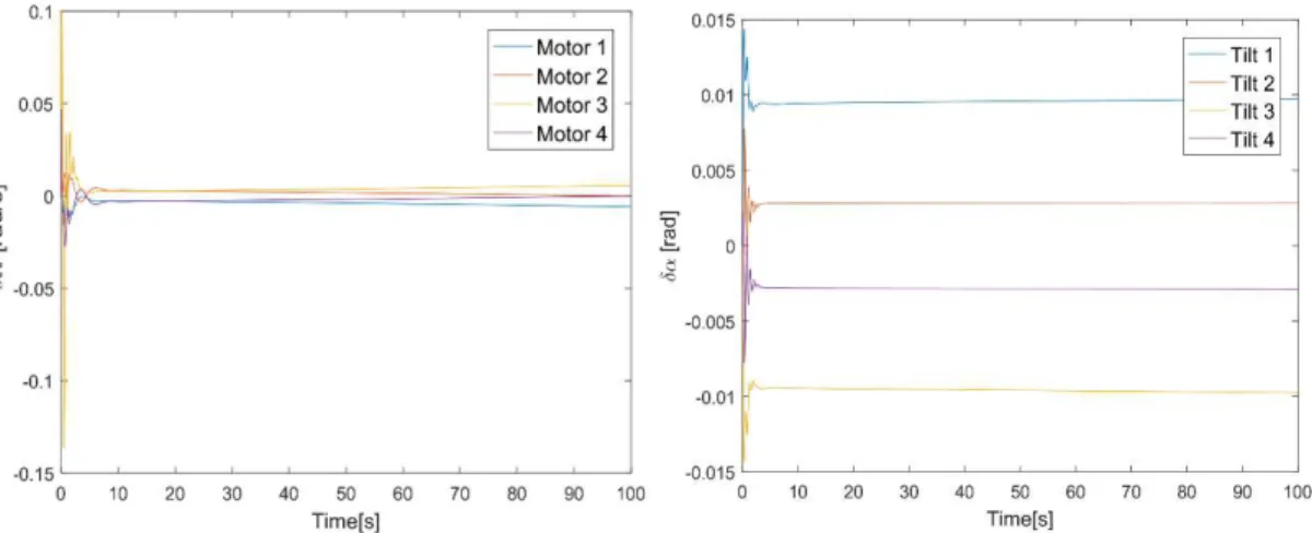
Figure 5.16 - Rotor angular speed (left) variation and tilt angle (right) when the multi-rotor has lateral tilting mechanism for a unit step on z direction.
Once the multi-rotor displacement on each inertial direction was investigated, the system behavior will be tested for a unitary step on all three directions simultaneously. The position and Euler angles responses are illustrated on Fig. 5.17 and 5.18, respectively and also the linear and angular velocities. Higher oscillations on the y-direction response when the system is not equipped with tilt mechanism.
66
Figure 5.17 - Multi-copter position (left) and velocity (right) for a unit step (purple) on the on all three directions x, y, and z for 3 different configurations: no tilt (blue), 4 longitudinal tilting mechanisms (red) and 4 lateral tilting mechanisms (yellow).
67
Figure 5.19 - Rotor angular speed variation when the multi-rotor has no tilting mechanism for a unit step on x, y and z directions.
69
5.3.1 Choice of Weighting Matrices
To design a controller for a second order derivative reference signal, the choice of the weighting matrices shall be different from the matrices presented on Eqs. (5.2.4), (5.2.6) and (5.2.7). Again, based on trial and error experience, the weighting matrices for the ramp reference signal will be:
0.5 0.5 10 5 5 10 0.1 0.1 0.2 250 25 5000 500 0.5 0.5 10
k
Q diag (5.3.1)
0.005 0.002 0.0008 0.0002
k
(5.3.2)
500 500 500 500
k
(5.3.3)
Comparing with the step weighting values from Eqs. (5.2.4), (5.2.6) and (5.2.7), more 3 lines and columns were added to the Qk matrix which represents the error second derivative terms. Also, comparing the weighting values considered with respect to the step input case, it is noted that the weighting values for the motors were decreased allowing higher values of angular input and the tilting values were increased to reduce the instabilities due high tilting angles.
Again, the stability of the system must be checked before making time response analysis. Since the stability variation were already checked for the number of tilting mechanisms, for now on, only three cases will be studied: no tilt, 4 longitudinal tilt, and 4 lateral tilt.
5.3.2 Poles and Zeros Analyses
On this case, likewise the analysis performed to the first order derivative controller (step input signal), the pole and zeros mapping has the objective to compare the system stability for the different actuation configuration and seek possible stability problems as the non-minimum- phase zeros.
70
Figure 5.22 - (Left) closed-loop poles for a second order integrator controller (ramp input signal), (Right) poles close to origin, for three actuator configurations: no tilt, 4 lateral tilt and 4 longitudinal tilt.
Figure 5.23 - (Left) closed-loop zeros for a second order integrator controller (ramp input signal), (Right) zeros close to origin, for three actuator configurations: no tilt, 4 lateral tilt and 4 longitudinal tilt.
71
5.3.3 Time Response Analysis
As soon as the multi-copter’s sensibility response for the three-spatial direction has already been tested for a step response, it would be redundant to verify it for other signals since the same discrepancies were presented such as: tilt actuation when performing an ascending flight and less oscillations on x and y directions.
Then, the system behavior will be investigated setting a unit ramp reference command to all three directions simultaneously representing a 3D ramp with 45 deg angle w.r.t. the ground (xE
-yEplane). Once again, the response is studied considering the three different tilting mechanisms as present on Figs 5.24 and 5.25.
Figure 5.24 - Multi-copter position (left) and velocity (right) for a unit ramp input signal on the on x, y and z directions (purple) for 3 different configurations: no tilt (blue), 4 longitudinal tilting mechanisms (red) and 4 lateral tilting mechanisms (yellow).
72
having the tilt mechanism is slightly faster for yE and zE directions. However, looking at the multi-copter linear velocity (Fig. 5.24 right) and Euler angles (Fig. 5.25 right) it is verified that the signals do not converge to a finite value for the cases where the aircraft is equipped with the tilting mechanism.
This is a classic example of the non-minimum phase effect on the system steady state response. Even that the system reaches the reference condition, its input signal continues rising along with the reference input signal, as can be seen on Figs. 5.27 and 5.28. Therefore, the system tends to become unstable as t . In conclusion, the tilt-mechanism may be used very carefully on unbounded reference signals such as the ramp input since it is a non-minimum phase system.
Figure 5.25 - Multi-copter position (left) and velocity (right) for a unit ramp input signal on the on all three directions (x, y, and z) for 3 different configurations: no tilt (blue), 4 longitudinal tilting mechanisms (orange) and 4 lateral tilting mechanisms (yellow).
73
Figure 5.26 - Rotor angular speed variation when the multi-rotor has no tilting mechanism for a unit ramp inputs on x, y and z directions.
74
Figure 5.28 - Rotor angular speed (left) variation and tilt angle (right) when the multi-rotor has lateral tilting mechanism for a unit ramp inputs on x, y and z directions.
5.4 Sinusoidal Input Signal
The third type of input reference signal to be tested is the sinusoidal or harmonic functions. As stated on Chapter 3, the harmonic signal is also a second order time derivative signal as presented on Table 3.1. The difference from the sinusoidal controller to the ramp input controller
is that the term 2
1 0
a is added to the expanded matrix (Eq. (3.3.8)) also in the control loop multiplying the tracking variables output signal in order to correct the phase lag of the system. Thus, on this case, the weighting matrices will be maintained from the previously simulation.
5.4.1 Poles and Zeros Analysis
Once more, a brief stability analysis is made mapping the poles and zeros position on the Real/Imaginary plane presented on Figs. 5.29 and 5.30.
75
Figure 5.29 - (Left) closed-loop poles for a second order integrator controller (sinusoidal input signal), (Right) poles close to origin, for three actuator configurations: no tilt, 4 lateral tilt and 4 longitudinal tilt.
Figure 5.30 - (Left) closed-loop zeros for a second order integrator controller (sinusoidal input signal), (Right) zeros close to origin, for three actuator configurations: no tilt, 4 lateral tilt and 4 longitudinal tilt.
5.4.2 Time Domain Analysis
76
input signal equation chosen for the simulations has amplitude and frequency, A0 1m 0 0.796 rad/s, respectively, and can be written on the time domain as:
0 0 0
( ) sin( )
r t A t (5.4.1)
being 0 the phase of the signal. Starting the analysis on the xE direction, 0 is set as 90 deg so that the generated signal represents a cosine signal. The initial yaw angle is set as 45 deg or 4 rad in order to evaluate the capacity of the controller to bring system to stability. Finally, the system state responses are presented on Figs. 5.31 and 5.32
Firstly, from Fig. 5.31 it can be verified that all the three cases (no tilt, 4-longitudinal tilt and 4-lateral tilt) the system can follow the harmonic input signal. On the yE direction, the oscillations are much higher when the system has none or 4-longitudinal tilting mechanisms. However, the oscillations on zE direction was higher when the 4-lateral tilting mechanism is equipped. Further, observing Fig. 5.32 (right), it can be noted that the pitch angle has also higher oscillations for none or 4-longitudinal tilting mechanisms cases. This could be cause of instability to the system for higher amplitude signals. Finally, from Fig. 5.32 (right), it is observed that the controller brings the yaw angle to zero position when the multi-copter has lateral tilting mechanism, while it remains around the initial value (45 deg or 4 rad) for the none or longitudinal cases.
77
Figure 5.32 - Multi-copter angular velocity (left) and position (right) for a sinusoidal input signal (purple) on the x direction for 3 different configurations: no tilt (blue), 4 longitudinal tilting mechanisms (red) and 4 lateral tilting mechanisms (yellow).
Regarding the input signals on Figs. 5.33, 5.34 and 5.35 the rotor angular speed input signals are quite the same for all three cases and that the tilting angles assume small values. This fact can be explained by the high weighting values on k. It must be stated that, trying higher weighting values, the system is very susceptible to gyroscopic effects and tends to destabilize. Further, the peak values at the beginning are explained by the fact that the system departs from the origin (
0
E
78
Figure 5.33 - Rotor angular speed variation when the multi-rotor has no tilting mechanism for a sinusoidal input on x direction.
79
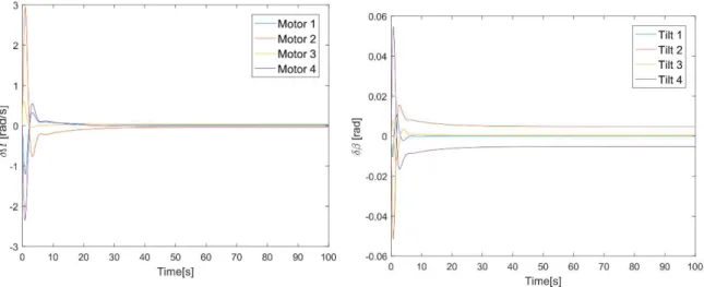
Figure 5.35 - Rotor angular speed (left) variation and tilt angle (right) when the multi-rotor has lateral tilting mechanism for a sinusoidal input on x direction.
Also, once again, the system response on the yE direction is expected to be the same due to the multi-rotor symmetry. Furthermore, the controller is not able to stabilize the response for a sinusoidal input on the zE direction with the same gain matrix.
Later, a circular trajectory reference signal on xE-yE plane is tested considering the
designed controller for the sinusoidal input. On this case, the initial yaw angle is set as zero. The circular reference equations on time domain are presented below:
0 0 0
( ) sin( )
x x x x
r t A t (5.4.2)
0 0 0
( ) sin( )
y y y y
r t A t (5.4.3)
( ) 0
z
r t (5.4.4)
In order to complete a circle, the parameters are set as 0x 0y 0.796rad/s, 0x 2
80
Figure 5.36 - Multi-copter position (left) and velocity (right) for a sinusoidal input signal (purple) on the x and y directions for 3 different configurations: no tilt (blue), 4 longitudinal tilting mechanisms (red) and 4 lateral tilting mechanisms (yellow).