The influence of the stratosphere on the tropospheric zonal wind response to CO<sub>2</sub> doubling

(1)

ACPD

10, 23895–23925, 2010

The stratosphere and CO₂ doubling

Y. B. L. Hinssen et al.

Title Page

Abstract Introduction

Conclusions References

Tables Figures

◭ ◮

Back Close

Full Screen / Esc

Printer-friendly Version

Interactive Discussion

Discussion

P

a

per

|

Dis

cussion

P

a

per

|

Discussion

P

a

per

|

Discussio

n

P

a

per

|

Atmos. Chem. Phys. Discuss., 10, 23895–23925, 2010 www.atmos-chem-phys-discuss.net/10/23895/2010/ doi:10.5194/acpd-10-23895-2010

Atmospheric Chemistry and Physics Discussions

This discussion paper is/has been under review for the journal Atmospheric Chemistry and Physics (ACP). Please refer to the corresponding final paper in ACP if available.

The influence of the stratosphere on the

tropospheric zonal wind response to CO

₂

doubling

Y. B. L. Hinssen1, C. J. Bell2,†, and P. C. Siegmund3

1

Institute for Marine and Atmospheric research Utrecht, Utrecht University, P.O. Box 80000, 3508 TA Utrecht, The Netherlands

2

Department of Meteorology, University of Reading, UK 3

Royal Netherlands Meteorological Institute – KNMI, De Bilt, The Netherlands †

deceased June 2010

Received: 11 August 2010 – Accepted: 22 September 2010 – Published: 12 October 2010

Correspondence to: Y. B. L. Hinssen (y.b.l.hinssen@uu.nl)

(2)

ACPD

10, 23895–23925, 2010

Title Page

Tables Figures

◭ ◮

Back Close

Full Screen / Esc

Discussion

P

a

per

|

Dis

cussion

P

a

per

|

Discussion

P

a

per

|

Discussio

n

P

a

per

|

Abstract

The influence of a CO2doubling on the stratospheric potential vorticity (PV) is

exam-ined in two climate models. Subsequently, the influence of changes in the stratosphere on the tropospheric zonal wind response is investigated, by inverting the stratospheric PV.

5

Radiative effects dominate the stratospheric response to CO2doubling in the

South-ern Hemisphere. These lead to a stratospheric PV increase at the edge of the polar vortex, resulting in an increased westerly influence of the stratosphere on the tropo-spheric midlatitude winds in late winter.

In the Northern Hemisphere, dynamical effects are also important. Both models

10

show a reduced polar PV and an enhanced midlatitude PV in the Northern Hemisphere winter stratosphere. These PV changes are related to an enhanced wave forcing of the winter stratosphere, as measured by an increase in the 100 hPa eddy heat flux, and result in a reduced westerly influence of the stratosphere on the high latitude tropo-spheric winds. In one model, the high latitude PV decreases are, however, restricted 15

to higher altitudes, and the tropospheric response due to the stratospheric changes is dominated by an increased westerly influence in the midlatitudes, related to the in-crease in midlatitude PV in the lower stratosphere.

The tropospheric response in zonal wind due to the stratospheric PV changes is of

the order of 0.5 to 1 m s−1. The total tropospheric response has a somewhat diff

er-20

ent spatial structure, but is of similar magnitude. This indicates that the stratospheric

influence is of importance in modifying the tropospheric zonal wind response to CO2

doubling.

1 Introduction

Numerous studies have examined model simulations of climate change due to increas-25

(3)

ACPD

10, 23895–23925, 2010

Title Page

Tables Figures

◭ ◮

Back Close

Full Screen / Esc

Discussion

P

a

per

|

Dis

cussion

P

a

per

|

Discussion

P

a

per

|

Discussio

n

P

a

per

|

a cooling of the stratosphere are observed in these simulations (e.g., Gillett et al., 2003; Sigmond et al., 2004; Bell et al., 2010). The response in the zonal wind is, however, sensitive to the changes in the horizontal temperature gradient, which shows more variability among models. Cooling in the polar lower stratosphere and warming in the tropical upper troposphere enhances the horizontal temperature gradient near 5

the midlatitude tropopause. Through the thermal wind relationship, this is related to increased westerly winds in the midlatitudes, in the tropopause region, but with a pos-sible downward influence toward the surface. There are indeed model studies that predict an increase in the Arctic Oscillation (AO) index, which is a measure for the tro-pospheric flow at midlatitudes, for increasing greenhouse gas concentrations (Shindell 10

et al., 1999; Gillett et al., 2002; Moritz et al., 2002). However, Baldwin et al. (2007) note that most climate models with a well-represented stratosphere indicate that the meridional overturning circulation in the stratosphere, the Brewer-Dobson circulation, will accelerate under climate change. This would lead to adiabatic warming and higher temperatures in the Arctic lower stratosphere, resulting in weaker westerly winds in 15

the Northern Hemisphere extratropics. Although the exact future response of the AO index is still uncertain, it is likely that stratospheric processes play a role in forming the tropospheric response to climate change.

Sigmond et al. (2004) performed simulations with a global climate model in which

the carbon dioxide (CO₂) concentration was separately doubled in the stratosphere,

20

the troposphere, and the entire atmosphere. They found that the CO2 doubling in the

entire atmosphere leads to an increase of the tropospheric midlatitude westerlies in the Northern Hemisphere winter, and that this increase in the troposphere is mainly due to

the CO2 doubling in the stratosphere. There are two ways by which stratospheric

cli-mate change due to increased CO2can have an effect on the troposphere, namely the

25

effect of stratospheric CO₂increase on the troposphere, and the effect of stratospheric

climate changes, due to tropospheric CO2increase, on the troposphere. Only the

for-mer effect was investigated by Sigmond et al. (2004). However, they also find that

(4)

ACPD

10, 23895–23925, 2010

Title Page

Tables Figures

◭ ◮

Back Close

Full Screen / Esc

Discussion

P

a

per

|

Dis

cussion

P

a

per

|

Discussion

P

a

per

|

Discussio

n

P

a

per

|

in the stratosphere and warming of the polar lower stratosphere in northern winter. It

is not yet known how this troposphere-induced stratospheric change affects the

tro-posphere. Or, more general, it is still a question what the effect is of stratospheric

climate change, indirectly due to CO2 increase in the troposphere and directly due to

CO₂ increase in the stratosphere, on the troposphere. This question is considered in

5

the present study. More specifically, we investigate the effect of stratospheric climate

change due to CO2increase in the entire atmosphere on the tropospheric wind, by

ap-plying piecewise potential vorticity (PV) inversion on the stratospheric PV in a reference

climatology and the stratospheric PV in a doubled CO2climatology.

This work is based on simulations with the middle-atmosphere version of the 10

ECHAM4 climate model as performed by Sigmond et al. (2004) and simulations with the Unified Model (UM), which is based on the Hadley Centre Atmosphere Model (HadAM3) coupled to a thermodynamic slab ocean model (Gillett et al., 2003). These models will be referred to as the “ECHAM model” and the “UM model”, respectively. For

both models, results from a control run and a run with doubled carbon dioxide (CO2)

15

concentrations are used. The studies of Sigmond et al. (2004) and Gillett et al. (2003)

describe the effect of CO₂ doubling in terms of temperature and wind changes. Bell

et al. (2010) further show that the doubled CO2response in the UM model is robust, as

a similar structure of the response, but with larger amplitude, is found under

quadru-pled CO₂ concentrations. Here we focus on changes in the stratospheric PV that are

20

related to CO2 doubling, and investigate to what extent these stratospheric changes

influence the tropospheric zonal mean zonal wind response.

Piecewise PV inversion (Davis, 1992) is used on a monthly basis to examine to what extent the zonal mean influence of the stratosphere on the tropospheric winds changes due to an increase in greenhouse gases. PV inversion makes use of the rela-25

(5)

ACPD

10, 23895–23925, 2010

Title Page

Tables Figures

◭ ◮

Back Close

Full Screen / Esc

Discussion

P

a

per

|

Dis

cussion

P

a

per

|

Discussion

P

a

per

|

Discussio

n

P

a

per

|

A change in the stratospheric PV due to an increase in CO₂might therefore affect the

tropospheric wind.

Section 2 presents an overview of the data used and a short description of the PV

inversion method. The influence of a CO₂ doubling on the stratospheric PV is

pre-sented in Sect. 3, while the influence of the stratosphere on the tropospheric zonal 5

wind response is studied in Sect. 4. Finally, some conclusions are given in Sect. 5.

2 Data and inversion method

The climatological PV is determined from the monthly mean temperature and zonal mean wind on 30 pressure levels between 1000 hPa and 0.01 hPa for the UM model,

where a 25-yr control run (pre-industrial CO₂ concentration of 289 ppmv) and a 25-yr

10

doubled CO2run are considered (Gillett et al., 2003). A zonal mean reconstruction of

pre-industrial ozone concentrations was prescribed, and the CO2concentrations were

kept constant within a run. The monthly mean data of the zonal wind and the temper-ature are interpolated from isobaric to isentropic levels with the method described by Edouard et al. (1997). Zonal averaging and averaging over the 25 years is performed 15

to obtain a climatological dataset of the zonal mean zonal wind and pressure on isen-tropic levels. In order to make optimal use of the data, a stretched grid in the vertical

direction is employed. The zonal mean isentropic potential vorticityZθ (Hoskins et al.,

1985) is then calculated from:

Zθ=

ζ_θ+f

σ (1)

20

Hereζθis the zonal mean isentropic relative vorticity,f is the Coriolis parameter andσ

is the isentropic density:

ζθ=−

1 a

∂u

∂φ+

utanφ

a (2)

σ=−1 g

∂p

(6)

ACPD

10, 23895–23925, 2010

Title Page

Tables Figures

◭ ◮

Back Close

Full Screen / Esc

Discussion

P

a

per

|

Dis

cussion

P

a

per

|

Discussion

P

a

per

|

Discussio

n

P

a

per

|

Hereuis the zonal mean zonal wind,θis the potential temperature, ais the radius of

the Earth, φis the latitude, p is the pressure and g is the gravitational acceleration.

This gives a climatological dataset of zonal mean PV, zonal wind and pressure on

isentropic levels. The domain of this dataset ranges from 90◦ to 10◦ north and south

(the tropical band is excluded, since the PV can occasionally be negative between the 5

equator and 10◦N and the PV inversion equation described below is not solvable then),

with a horizontal resolution of 2.5◦, and from the lower troposphere to about 1250 K in

the vertical, with a resolution varying from about 2 K in the troposphere to 10 K in the upper layers. The lower boundary for each latitude is defined as the lowest isentropic level for which data is available along the full latitude circle (meaning that the pressure 10

is below 1000 hPa at all longitudes along this latitude circle). We will refer to this lower boundary as the “surface”, but it should be noted that this does not correspond to the actual surface of the Earth, but is located in the lower or middle troposphere.

Similarly, the climatological PV is determined from the monthly mean temperature and zonal mean wind on 33 pressure levels between 1000 hPa and 0.01 hPa for the 15

ECHAM model, where the last 20 years of both the control run (CO2concentration of

353 ppmv, note that this concentration is higher than in the UM model) and the doubled

CO2 run are considered (Sigmond et al., 2004). As stated in Sigmond et al. (2004),

the ozone distribution is prescribed. The horizontal resolution of the ECHAM model is

about 2.8◦ (T42 horizontal resolution), and the data is interpolated to the same

isen-20

tropic levels as the UM model data.

The European Centre for Medium-Range Weather Forecasts (ECMWF) ERA-interim reanalysis data on 37 pressure levels between 1000 hPa and 1 hPa, and a horizontal

resolution of 1.5◦ is used for comparison with the model results. The monthly mean

data (at 12:00 UTC) of the zonal wind and the temperature for the period 1989 to 2008 25

are again interpolated from isobaric to isentropic levels. Zonal averaging and

averag-ing over the 20 years is performed to obtain a climatological dataset of u and p on

(7)

ACPD

10, 23895–23925, 2010

Title Page

Tables Figures

◭ ◮

Back Close

Full Screen / Esc

Discussion

P

a

per

|

Dis

cussion

P

a

per

|

Discussion

P

a

per

|

Discussio

n

P

a

per

|

The relation between the potential vorticity and the zonal wind is given by the PV in-version equation, which is derived from the definition of the isentropic potential vorticity given in Eq. (1) and the conditions of hydrostatic balance and gradient wind balance between the zonal mean zonal wind, temperature and pressure. The PV inversion equation reads (see also Hinssen et al., 2010b):

5

Z_θ g

∂ ∂θ

ρθfloc

∂u ∂θ

+∂

2 u ∂r2+

tanφ

a ∂u

∂r −

u

a2_cos2_φ=σ ∂Z_θ

∂r −

∂f

∂r (4)

with

floc=f(r)+

2tanφ

a u;r=a

π

2−φ

;f(r)=2Ωsinφ=2Ωcosr

a

(5)

Here,r is the distance from the pole measured along the surface of the Earth,ρis the

density (derived from the equation of state) andΩis the rotation rate of the Earth.

10

The PV inversion equation, Eq. (4), can be seen as the formulation of thermal wind balance in terms of potential vorticity. It describes the flow pattern that is associated with a specific pattern of the potential vorticity in a balanced axi-symmetric vortex cen-tred at the pole.

The boundary condition at the pole (r=0) is simply thatu=0, because the vortex is

15

assumed to be axi-symmetric and centred at the pole. At the outer boundary, at 10◦, we

prescribe the wind according to the circulation theorem (Hoskins et al., 1985, p. 897). At the upper boundary we impose the ERA-interim wind or the modeled wind. Since we only consider inversion of the stratospheric PV distribution, zero thermal wind is imposed at the lower boundary:

20

∂u

∂θ =0 (6)

(8)

ACPD

10, 23895–23925, 2010

Title Page

Tables Figures

◭ ◮

Back Close

Full Screen / Esc

Discussion

P

a

per

|

Dis

cussion

P

a

per

|

Discussion

P

a

per

|

Discussio

n

P

a

per

|

Zero thermal wind is, however, believed to be a reasonable boundary condition for the inversion of the stratospheric part of the PV. PV inversion is performed on the monthly PV values between 400 K and 1250 K, by solving Eq. (4) by successive relaxation.

On the basis of the PV inversion equation, the zonal mean PV and the isentropic density are split into a reference state and an anomaly as follows:

5

Z_θ≡Z_θ,_ref+Z_θ′;σ≡σ_ref+σ′ (7)

with

Zθ,ref= f σref

(8)

and

σref= R

σcos(φ)d φ R

cos(φ)d φ (9)

10

In other words, the reference isentropic densityσrefis the area-weighted average ofσ

over the domain in question. In our case we choose the area poleward of 10◦.

There-fore,σrefdepends only onθ. The reference PV is associated with the solutionu=0 and

σ=σref, indicating that the PV anomaly represents that part of the PV field that induces

a wind field, according to the PV inversion equation. With this definition two sepa-15

rate PV anomalies centred over the pole are distinguished: one at the tropopause and the other in the polar night stratosphere at potential temperatures above about 400 K (Hinssen et al., 2010b). In this study, we examine the influence of the stratospheric polar cap PV anomaly between 400 K and 1250 K on the tropospheric winds, since the

PV anomaly in this altitude range is most affected by CO2 doubling. The total PV is

20

used for the inversion, but the PV anomaly will be discussed in relation to the resulting wind field, since only variations in the PV anomaly are associated with variations in the wind field.

(9)

ACPD

10, 23895–23925, 2010

Title Page

Tables Figures

◭ ◮

Back Close

Full Screen / Esc

Discussion

P

a

per

|

Dis

cussion

P

a

per

|

Discussion

P

a

per

|

Discussio

n

P

a

per

|

stratosphere (100 hPa) is therefore often used as a measure of the wave forcing from the troposphere to the stratosphere (see also Waugh et al., 1999; Polvani and Waugh,

2004; Charlton et al., 2007). The monthly heat flux [v∗T∗] (a star represents a deviation

from the zonal mean quantity and the brackets indicate zonal averaging) is determined

from the monthly mean meridional wind (v) and temperature on pressure levels for

5

every year, for the models as well as for the ERA-interim data. In the next section, it is shown that the heat flux calculated from the monthly mean data gives a reasonable estimate of the seasonal cycle of the heat flux calculated from daily data. The

area-weighted average heat flux at 100 hPa is determined between 40◦ and 80◦ for both

hemispheres, since most wave activity enters the stratosphere in this latitude band. 10

The climatological flux values are determined by averaging over all years (20 years for the ERA-interim data and the ECHAM model, 25 years for the UM model).

3 Stratospheric PV changes

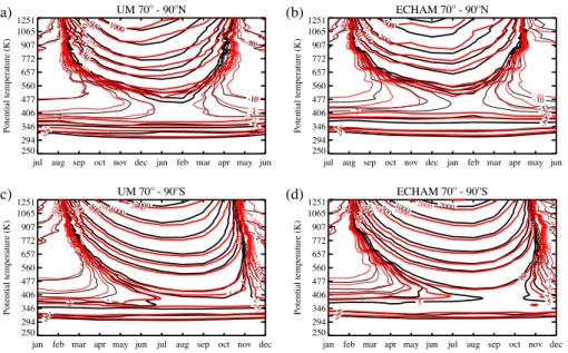
Figure 1 presents the polarcap PV anomaly, defined as the area-weighted average

isentropic PV anomaly between 70◦and 90◦, for the control runs (in black) and for the

15

doubled CO2runs (red), for both hemispheres. The polar PV anomaly is studied since

the zonal wind field is related to horizontal gradients in PV (the first term on the right hand side of Eq. (4) involves the horizontal PV gradient), so that changes in the polar

PV can affect the midlatitude winds. Comparison of the ERA-interim data to the model

data (not shown) indicates that the model results are realistic, in amplitude as well as 20

in seasonal cycle. Both models show a similar polarcap PV response to CO2doubling.

The Northern Hemisphere (NH) polar stratospheric PV increases somewhat in autumn

and spring due to CO₂doubling, while it decreases in winter. An increase in Southern

Hemisphere (SH) polar stratospheric PV is found from autumn through spring. These PV changes are consistent with the results of Butchart et al. (2000), who find enhanced 25

(10)

ACPD

10, 23895–23925, 2010

Title Page

Tables Figures

◭ ◮

Back Close

Full Screen / Esc

Discussion

P

a

per

|

Dis

cussion

P

a

per

|

Discussion

P

a

per

|

Discussio

n

P

a

per

|

The stratospheric polarcap PV at 600 K is shown in Fig. 2a and b, for the UM model and ECHAM model, respectively. At 600 K the midwinter PV response is largest in the UM model. This is also true at higher levels in autumn and spring, while at higher levels the NH midwinter PV changes are somewhat larger in the ECHAM model than in the UM model (Fig. 1).

5

The midlatitude PV anomaly (area-weighted average PV anomaly between 35◦ and

55◦) at 600 K is given in Fig. 2c (UM model) and d (ECHAM model). The NH polarcap

PV anomaly decreases in winter due to CO₂ doubling, while the NH midlatitude PV

anomaly increases (the amplitude of the seasonal cycle decreases in both cases),

indicating increased wave breaking, mixing PV offthe pole (McIntyre and Palmer, 1983,

10

1984). In the SH, the polarcap PV anomaly increases, and a slight decrease in the midlatitude PV is found throughout most of the year, with an increase in winter in the ECHAM model.

The stratospheric PV distribution is determined by radiative effects and wave effects.

Since the ozone concentrations are kept fixed in the models, the PV differences

be-15

tween the control run and the doubled CO2 run are not related to ozone variations.

The change in CO₂ has a radiative effect. A higher stratospheric CO₂ concentration

will lead to an enhanced cooling to space (Fels et al., 1980; Butchart et al., 2000; Shin-dell et al., 2001), and an accompanying increase in stratospheric PV. This is indeed seen in the SH (Figs. 1c and d and 2a and b), and in NH autumn and spring, but not in 20

NH winter.

CO2 doubling can also influence the wave forcing. Eichelberger and Hartmann

(2005), for example, show that an increase in the meridional temperature gradient (due to tropical upper tropospheric warming or polar lower stratospheric cooling) could lead to enhanced baroclinicity in the midlatitudes and enhanced baroclinic wave generation. 25

(11)

ACPD

10, 23895–23925, 2010

Title Page

Tables Figures

◭ ◮

Back Close

Full Screen / Esc

Discussion

P

a

per

|

Dis

cussion

P

a

per

|

Discussion

P

a

per

|

Discussio

n

P

a

per

|

To examine the extent to which the wave forcing can explain the PV response, the

area-weighted averaged 100 hPa monthly eddy heat flux between 40◦and 80◦is shown

in Fig. 3. Additionally, the ERA-interim 100 hPa heat flux is given in Fig. 4. The heat flux derived from the monthly mean data is lower than the monthly averages of the heat flux derived from daily data, but the seasonal cycle is similar. This indicates that the 5

monthly mean data is suitable to obtain an estimate of the seasonal cycle of the heat flux. The NH winter heat flux is somewhat higher for the ECHAM model than for the UM model. Interestingly, this is consistent with the ECHAM polarcap PV being somewhat

lower than the UM polarcap PV. CO2doubling hardly affects the SH heat flux in the UM

model, and leads to a slight decrease in the SH flux in autumn and spring in the ECHAM 10

model. The NH heat flux, on the other hand, increases in both models, especially in winter. The largest increase is found in December and January in the UM model, and in January and February in the ECHAM model. An increase in the NH upward flux of wave activity from the troposphere due to an increase in greenhouse gas concentrations is also found by, for example, Butchart et al. (2000), Schnadt et al. (2002) and Shepherd 15

(2008). Haklander et al. (2008) studied changes in the NH upward wave flux in the same ECHAM model runs in more detail, and found an increase of about 12% in the

January-February mean 100 hPa heat flux due to CO2 doubling. They state that this

can mainly be attributed to changes in stationary wave-1, related to an increase in the meridional temperature gradient, and suggest that at least part of the increase is 20

due to more stationary wave-1 generation at midlatitudes in the troposphere. Sigmond

et al. (2004) show that tropospheric CO2 doubling alone results in a warming of the

lower polar stratosphere in the NH winter. This warming is likely related to the wave forcing (through an increase in the Brewer-Dobson circulation), suggesting that the

heat flux increase in the NH is related to the CO2doubling in the troposphere. Changes

25

initially made to the troposphere (increase in CO₂) could thus affect the stratospheric

(12)

ACPD

10, 23895–23925, 2010

Title Page

Tables Figures

◭ ◮

Back Close

Full Screen / Esc

Discussion

P

a

per

|

Dis

cussion

P

a

per

|

Discussion

P

a

per

|

Discussio

n

P

a

per

|

A stronger winter wave forcing is related to lower polarcap PV anomaly values and higher midlatitude PV anomaly values (Hinssen et al., 2010a), similar to what is found

for a CO2 doubling in the NH (Fig. 2). The increase in midlatitude winter stratospheric

PV in the SH ECHAM model is likely related to the polar cooling and the accompany-ing increase in polar PV, extendaccompany-ing further equatorward than in the control run, thereby 5

also affecting the midlatitude PV. If this effect plays a role, it is expected to do so in late

winter, when the vortex attains its maximum size at the 600 K level. For the ECHAM model, the decrease in midlatitude PV in autumn and spring could be related to the decrease in wave forcing (Fig. 3b), but this decrease in wave forcing is absent in the UM model, indicating that other processes must play a role as well. Other processes 10

may incorporate changes in the propagation and absorption of waves within the strato-sphere. Several studies have shown that waves tend to propagate more toward the equator for stronger westerly winds in the lower stratosphere (Hartmann et al., 2000; Shindell et al., 2001; Perlwitz and Harnik, 2003; Kushner and Polvani, 2004; Sigmond and Scinocca, 2010). Planetary wave refraction is influenced by wind shear. Waves 15

propagating upward from the troposphere are refracted equatorward by the increased vertical wind shear in the lower stratosphere when the vortex is strong (Shindell et al., 2001). This provides a positive feedback, where a stronger vortex is less disturbed

by waves. A strengthening of the SH vortex due to CO2 doubling might thus lead to

more equatorward refraction of waves, an increase in the polarcap PV anomaly and 20

a decrease in the PV anomaly at lower latitudes, since less polar PV is transported off

the pole.

4 Stratospheric influence on the troposphere

Figures 1 and 2 displayed that a CO2doubling affects the stratospheric PV distribution.

To investigate the impact on the tropospheric circulation, PV inversion is applied to the 25

(13)

ACPD

10, 23895–23925, 2010

Title Page

Tables Figures

◭ ◮

Back Close

Full Screen / Esc

Discussion

P

a

per

|

Dis

cussion

P

a

per

|

Discussion

P

a

per

|

Discussio

n

P

a

per

|

in the upper stratosphere in autumn, reaching the lower stratosphere in winter (Fig. 1). Since it is mainly the lower stratosphere that influences the tropospheric winds, the late winter season is examined: February in the NH and August in the SH.

Since we consider climate change experiments, difficulties arise with interpreting the

wind response in isentropic coordinates. Globally averaged, a tropospheric warming 5

response of about 3 K is found, indicating a shift of the atmosphere relative to the po-tential temperature axis. A certain isentropic level in the troposphere will therefore be

closer to the surface for the doubled CO₂ run than for the control run. This means

that the wind response in isentropic coordinates mainly shows the tropospheric verti-cal wind shear, and not the change in winds due to climate change. Therefore it was 10

decided to interpolate the results back to pressure levels, to facilitate a fair compari-son of the wind response in the model runs and in the inversion results. Due to the interpolations and due to the way we define the lower boundary on isentropic levels (see Sect. 2), no results are available on the lowermost pressure levels. This, however, still allows us to examine the influence of the stratosphere on the middle troposphere, 15

which is suitable for the purpose of the present study.

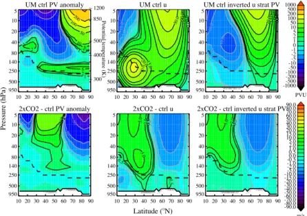
Figure 5 shows the NH February mean PV anomaly and zonal mean zonal wind field for the UM control run (top row, left and middle column) and the response to

CO2doubling (lower row). The approximate variation of the potential temperature with

pressure is indicated to the right of the upper left panel, where it should be noted that 20

the potential temperature strongly varies with latitude in the troposphere, at 500 hPa from about 280 K at the pole to 320 K in the tropics. The tropopause has a potential

temperature of about 300 K at the pole and 380 K at 10◦in winter, so the PV anomaly

above 400 K is indeed a stratospheric PV anomaly.

In the UM model, CO2 doubling results in a clear decrease in the PV anomaly

25

(14)

ACPD

10, 23895–23925, 2010

Title Page

Tables Figures

◭ ◮

Back Close

Full Screen / Esc

Discussion

P

a

per

|

Dis

cussion

P

a

per

|

Discussion

P

a

per

|

Discussio

n

P

a

per

|

inversion of the stratospheric PV above 400 K is shown in the right column of Fig. 5.

The stratospheric PV changes induce stratospheric wind changes, but also affect the

high latitude tropospheric winds (lower right panel in Fig. 5). The tropospheric wind

response related to the stratospheric PV changes is small (of the order of 0.5 m s−1),

but of the same order of magnitude as the total response in model zonal wind (lower 5

middle panel in Fig. 5). This indicates that the influence of the stratosphere is relevant for the tropospheric response, and that it results in a weaker westerly wind in the high latitude troposphere in the NH winter.

The results for the ECHAM model are presented in Fig. 6. The models agree on the

large scale response to CO2doubling. Both show a decrease in the polar stratospheric

10

PV, a decrease in the high latitude winds and an equatorward shift of the stratospheric polar jet. However, for the ECHAM model, the decrease in westerly winds in the strato-spheric inversions is restricted to the higher latitude stratosphere (lower right panel in

Fig. 6), while an increased westerly influence (of 0.5 to 1 m s−1) of the stratosphere on

the midlatitude tropospheric winds is found. Decreased PV anomaly values are indeed 15

restricted to somewhat higher latitudes and levels in the ECHAM model than in the UM model, while an increase in the mid- to high latitude PV anomaly is found in the lower stratosphere in the ECHAM model (compare the lower left panels of Figs. 5 and 6). These figures illustrate that a slight shift in the location of a PV anomaly (in altitude or latitude) can change the tropospheric response to stratospheric PV changes.

20

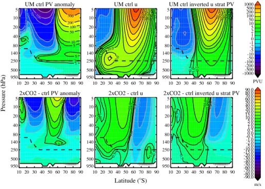
The SH August mean PV anomaly, wind field and inverted wind field from the strato-spheric PV are shown in Fig. 7 and 8 for the UM model and the ECHAM model,

re-spectively. Similar to Fig. 5, results are presented for the control run and the difference

between the doubled CO2 run and the control run. In the SH, both models show an

increase in the stratospheric PV anomaly around 55◦, while the low latitude and polar

25

PV anomaly values decrease. In both models the stratospheric PV differences have

(15)

ACPD

10, 23895–23925, 2010

Title Page

Tables Figures

◭ ◮

Back Close

Full Screen / Esc

Discussion

P

a

per

|

Dis

cussion

P

a

per

|

Discussion

P

a

per

|

Discussio

n

P

a

per

|

to the NH, an equatorward shift of the polar jet is also seen in the SH response. It should be noted that the PV anomalies shown in Figs. 5 to 8 are the isentropic PV values interpolated to pressure coordinates. In general the same features are observed in both coordinate systems, but an exception is the polar stratospheric PV anomaly in

the SH, which shows a decrease due to CO2 doubling on pressure levels in August

5

(Figs. 7 and 8), while an increase was observed on isentropic levels (Fig. 2a and b). This is related to a decrease in pressure on isentropic levels over the south pole due

to CO2doubling, while CO2doubling hardly affects the pressure over the north pole (in

February at 600 K). The stratospheric polar PV response in the NH is therefore similar on pressure levels and on isentropic levels.

10

In the previous section, the interpretation of the PV response to CO₂ doubling was

given on isentropic levels, since we consider the isentropic PV. It should however be kept in mind that the interpretation of a response to climate change depends on the coordinate system that is used.

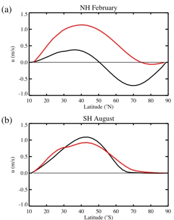
The tropospheric response related to changes in the stratospheric PV is summarized 15

in Fig. 9, which shows the wind response in the middle troposphere, at 400 hPa, for February in the NH (Fig. 9a) and for August in the SH (Fig. 9b). In the UM model, there

is an easterly response on the tropospheric winds north of 50◦N, while the response

is westerly at low northern latitudes. The ECHAM model gives a westerly response

south of 70◦N and hardly any response at the high northern latitudes. In the SH, both

20

models give a similar westerly response equatorward of about 65◦S, maximizing at

1 m s−1around 40◦S.

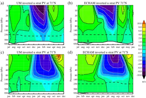
The previous results were for the late winter season. Figure 10 indicates how the wind response, obtained from inverting the stratospheric PV, changes throughout the

year, as a function of pressure, at 71◦.

25

In the UM model, the NH tropospheric wind response to the stratospheric PV changes is small throughout the year, with a slightly decreased westerly influence in late winter and a slightly increased westerly influence in summer. For the NH

(16)

ACPD

10, 23895–23925, 2010

Title Page

Tables Figures

◭ ◮

Back Close

Full Screen / Esc

Discussion

P

a

per

|

Dis

cussion

P

a

per

|

Discussion

P

a

per

|

Discussio

n

P

a

per

|

stratosphere on the high latitude tropospheric winds from summer to early winter and in early spring, while a decreased westerly influence is found in late winter.

A slight decrease in the westerly influence is found in the winter season in the SH as

well. The SH response to CO2doubling is an increased westerly influence of the

strato-sphere on the midlatitude tropospheric winds of the order of 0.5 to 1 m s−1throughout

5

the year (not shown), but at the high latitudes this increased westerly influence is re-stricted to the summer and autumn seasons (Fig. 10c and d).

For comparison, Fig. 11 shows the total wind response in the model runs, again at

71◦. The figures presented in this section show that the tropospheric wind response

due to changes in the stratospheric PV is small, of the order of 0.5 to 1 m s−1, but also

10

indicate that the total wind response in the model is of the same order of magnitude. The stratospheric influence is therefore not negligible. The tropospheric response in the models is sometimes of opposite sign as the response to stratospheric PV changes, indicating that tropospheric processes can modify and mask the stratospheric influ-ence.

15

5 Conclusions

We examined the influence of a CO₂ doubling on the zonal mean stratospheric PV

distribution for the UM model (based on the Hadley Centre Atmosphere Model cou-pled to a thermodynamic slab ocean model) and the middle-atmosphere version of the ECHAM4 climate model. Subsequently, we investigated the tropospheric wind re-20

sponse to changes in the stratospheric PV, by inverting the stratospheric PV.

An increase in greenhouse gases enhances the stratospheric emission of longwave radiation and the cooling to space. Based on these radiative arguments, an increase in the stratospheric PV is expected. This is indeed found in the SH winter, but not in the NH, indicating that other processes are of importance as well. Inspection of the 25

100 hPa eddy heat flux, used as a measure of the wave forcing from the troposphere

to the stratosphere, shows an increased winter flux in the NH due to CO2 doubling.

(17)

in-ACPD

10, 23895–23925, 2010

Title Page

Tables Figures

◭ ◮

Back Close

Full Screen / Esc

Discussion

P

a

per

|

Dis

cussion

P

a

per

|

Discussion

P

a

per

|

Discussio

n

P

a

per

|

creased heat flux is associated with a reduced polarcap PV anomaly and an enhanced midlatitude PV anomaly. In autumn and spring the change in heat flux is small and the

NH polar PV slightly increases, likely related to the cooling effect of the increased CO2

concentrations. In the SH, a CO2doubling hardly affects the 100 hPa heat flux, and the

radiative effect dominates, leading to an increase in the polar PV on isentropic levels.

5

The influence of the stratospheric PV on the tropospheric wind depends on the PV in

the lower stratosphere. Due to CO2doubling, the SH lower stratospheric PV increases

in late winter. An increased westerly influence of the stratosphere on the tropospheric midlatitude winds is therefore found in August, in both models. The largest PV in-creases are found in midlatitudes, at the edge of the vortex. The horizontal gradient in 10

PV thus increases in the midlatitudes, leading to increased westerlies, but the horizon-tal PV gradient decreases at high latitudes, leading to somewhat decreased westerlies

there, mainly in the stratosphere. In the NH, CO2 doubling is associated with a

de-crease in the stratospheric PV in late winter, resulting in a reduced westerly influence of the stratospheric PV on the high latitude tropospheric winds. In the ECHAM model, 15

the decrease in stratospheric PV is, however, restricted to higher altitudes than in the UM model, and an increased westerly influence is found in the low to midlatitudes, related to the increase in midlatitude PV in the lower stratosphere.

The tropospheric response in zonal wind due to stratospheric PV changes is of the

order of 0.5 to 1 m s−1. The tropospheric wind response obtained from the

strato-20

spheric inversions differs in structure from the total tropospheric wind response, but is

of similar magnitude, indicating that changes in the stratosphere can certainly modify

the tropospheric wind response to CO₂doubling.

The present study shows that although radiative effects of greenhouse gases are

important in determining the stratospheric PV distribution, it can not simply be assumed 25

that the stratospheric PV increases with increasing greenhouse gas concentrations,

since the wave forcing of the stratosphere might also change due to increases in CO2.

The results presented here indicate that, in the NH, the wave effect might dominate over

(18)

ACPD

10, 23895–23925, 2010

Title Page

Tables Figures

◭ ◮

Back Close

Full Screen / Esc

Discussion

P

a

per

|

Dis

cussion

P

a

per

|

Discussion

P

a

per

|

Discussio

n

P

a

per

|

influence of the stratosphere on the tropospheric response to climate change depends very sensitive on the radiatively and dynamically induced PV changes in the lower stratosphere. This is consistent with the studies of Sigmond et al. (2008) and Sigmond and Scinocca (2010), who found that the state of the lower stratosphere influences the tropospheric response to climate change, and that a low model top, in the middle 5

stratosphere, is sufficient to capture the stratospheric influence.

Acknowledgements. The ECMWF ERA-interim data used in this study have been provided

by ECMWF. The ECHAM model data were made available by Alwin Haklander at KNMI, and Michael Sigmond at the University of Toronto. We thank Theo Opsteegh and Aarnout van Delden for useful discussions.

10

References

Baldwin, M. P., Dameris, M., and Shepherd, T. G.: How will the stratosphere affect climate

change?, Science, 316, 1576–1577, 2007. 23897

Bell, C. J., Gray, L. J., and Kettleborough, J.: Changes in Northern Hemisphere stratospheric

variability under increased CO₂ concentrations, Q. J. Roy. Meteor. Soc., 136, 1181–1190,

15

2010. 23897, 23898

Black, R. X.: Stratospheric forcing of surface climate in the Arctic Oscillation, J. Climate, 15, 268–277, 2002. 23898

Black, R. X. and McDaniel, B. A.: Diagnostic case studies of the Northern Annular Mode, J. Climate, 17, 3990–4004, 2004. 23898

20

Butchart, N. and Scaife, A. A.: Removal of chlorofluorocarbons by increased mass exchange between the stratosphere and troposphere in a changing climate, Nature, 410, 799–802, 2001. 23904

Butchart, N., Austin, J., Knight, J. R., Scaife, A. A., and Gallani, M. L.: The response of the stratospheric climate to projected changes in the concentrations of well-mixed greenhouse 25

gases from 1992 to 2051, J. Climate, 13, 2142–2159, 2000. 23903, 23904, 23905

(19)

ACPD

10, 23895–23925, 2010

Title Page

Tables Figures

◭ ◮

Back Close

Full Screen / Esc

Discussion

P

a

per

|

Dis

cussion

P

a

per

|

Discussion

P

a

per

|

Discussio

n

P

a

per

|

Davis, C. A.: Piecewise potential vorticity inversion, J. Atmos. Sci., 49, 1397–1411, 1992. 23898 Edouard, S., Vautard, R., and Brunet, G.: On the maintenance of potential vorticity in isentropic

coordinates, Q. J. Roy. Meteor. Soc., 123, 2069–2094, 1997. 23899

Eichelberger, S. J. and Hartmann, D. L.: Changes in the strength of the Brewer-Dobson cir-culation in a simple AGCM, Geophys. Res. Lett., 32, L15807, doi:10.1029/2005GL022924, 5

2005. 23904

Fels, S. B., Mahlman, J. D., Schwarzkopf, M. D., and Sinclair, R. W.: Stratospheric sensitivity to perturbations in ozone and carbon dioxide: radiative and dynamical response, J. Atmos. Sci., 37, 2265–2297, 1980. 23904

Gillett, N. P., Allen, M. R., McDonald, R. E., Senior, C. A., Shindell, D. T., and Schmidt, G. A.: 10

How linear is the Arctic Oscillation response to greenhouse gases?, J. Geophys. Res., 107(D3), 4022, doi:10.1029/2001JD000589, 2002. 23897

Gillett, N. P., Allen, M. R., and Williams, K. D.: Modelling the atmospheric response to doubled

CO₂ and depleted stratospheric ozone using a stratosphere-resolving coupled GCM, Q. J.

Roy. Meteor. Soc., 129, 947–966, doi:10.1256/qj.02.102, 2003. 23897, 23898, 23899 15

Haklander, A. J., Siegmund, P. C., Sigmond, M., and Kelder, H. M.: How does the

northern-winter wave driving of the Brewer-Dobson circulation increase in an enhanced-CO₂climate

simulation?, Geophys. Res. Lett., 35, L07702, doi:10.1029/2007GL033054, 2008. 23905 Hartley, D. E., Villarin, J. T., Black, R. X., and Davis, C. A.: A new perspective on the dynamical

link between the stratosphere and troposphere, Nature, 391, 471–474, 1998. 23898 20

Hartmann, D. L., Wallace, J. M., Limpasuvan, V., Thompson, D. W. J., and Holton, J. R.: Can ozone depletion and global warming interact to produce rapid climate change?, P. Natl. Acad. Sci. USA, 97, 1412–1417, 2000. 23906

Hinssen, Y., van Delden, A., and Opsteegh, T.: The seasonal cycle of the potential vorticity distribution in the stratosphere, Q. J. Roy. Meteor. Soc., submitted, 2010a. 23906

25

Hinssen, Y., van Delden, A., Opsteegh, T., and de Geus, W.: Stratospheric impact on tropo-spheric winds deduced from potential vorticity inversion in relation to the Arctic Oscillation, Q. J. Roy. Meteor. Soc., 136, 20–29, doi:10.1002/qj.542, 2010b. 23898, 23901, 23902 Hoskins, B. J., McIntyre, M. E., and Robertson, A. W.: On the use and significance of isentropic

potential vorticity maps, Q. J. Roy. Meteor. Soc., 111, 877–946, 1985. 23898, 23899, 23901 30

Kleinschmidt, E.: ¨Uber Aufbau und Entstehung von Zyklonen, Meteorol. Rundsch., 3, 1–6,

1950. 23898

(20)

ACPD

10, 23895–23925, 2010

Title Page

Tables Figures

◭ ◮

Back Close

Full Screen / Esc

Discussion

P

a

per

|

Dis

cussion

P

a

per

|

Discussion

P

a

per

|

Discussio

n

P

a

per

|

AGCM: the role of eddies, J. Climate, 17, 629–639, 2004. 23906

McIntyre, M. E. and Palmer, T. N.: Breaking planetary waves in the stratosphere, Nature, 305, 593–600, 1983. 23904

McIntyre, M. E. and Palmer, T. N.: The “surf zone” in the stratosphere, J. Atmos. Terr. Phys., 46, 825–849, 1984. 23904

5

Moritz, R. E., Bitz, C. M., and Steig, E. J.: Dynamics of recent climate change in the Arctic, Science, 297, 1497–1502, 2002. 23897

Perlwitz, J. and Harnik, N.: Observational evidence of a stratospheric influence on the tropo-sphere by planetary wave reflection, J. Climate, 16, 3011–3026, 2003. 23906

Polvani, L. M. and Waugh, D. W.: Upward wave activity flux as a precursor to extreme strato-10

spheric events and subsequent anomalous surface weather regimes, J. Climate, 17, 3548– 3554, 2004. 23903

Schnadt, C., Dameris, M., Ponater, M., Hein, R., Grewe, V., and Steil, B.: Interaction of at-mospheric chemistry and climate and its impact on stratospheric ozone, Clim. Dynam., 18, 501–517, 2002. 23905

15

Shepherd, T. G.: Dynamics, stratospheric ozone, and climate change, Atmos. Ocean, 46, 117– 138, doi:10.3137/ao.460106, 2008. 23905

Shindell, D. T., Miller, R. L., Schmidt, G. A., and Pandolfo, L.: Simulation of recent northern winter climate trends by greenhouse-gas forcing, Nature, 399, 452–455, 1999. 23897 Shindell, D. T., Schmidt, G. A., Miller, R. L., and Rind, D.: Northern Hemisphere winter climate 20

response to greenhouse gas, ozone, solar, and volcanic forcing, J. Geophys. Res., 106, 7193–7210, 2001. 23904, 23906

Sigmond, M. and Scinocca, J. F.: The influence of the basic state on the

north-ern hemisphere circulation response to climate change, J. Climate, 23, 1434–1446, doi:10.1175/2009JCLI3167.1, 2010. 23906, 23912

25

Sigmond, M., Siegmund, P. C., Manzini, E., and Kelder, H.: A simulation of the separate climate

effects of middle-atmospheric and tropospheric CO₂ doubling, J. Climate, 17, 2352–2367,

2004. 23897, 23898, 23900, 23905

Sigmond, M., Scinocca, J. F., and Kushner, P. J.: Impact of the stratosphere on tropospheric climate change, Geophys. Res. Lett., 35, L12706, doi:10.1029/2008GL033573, 2008. 23912 30

(21)

ACPD

10, 23895–23925, 2010

Title Page Abstract Introduction Conclusions References Tables Figures ◭ ◮ ◭ ◮ Back Close

Full Screen / Esc

Printer-friendly Version Interactive Discussion Discussion P a per | Dis cussion P a per | Discussion P a per | Discussio n P a per |

jul aug sep oct nov dec jan feb mar apr may jun 250 294 346 406 477 560 657 772 907 1065 1251

Potential temperature (K)

UM 70O

- 90O

N -50 -50 -10 -10 -5 -5 -2 -2 -2 2 2 2 2 5 5 5 5 10 50 100200 500 1000 -50 -50 -1 0 -10 -5 -5 -2 -2 2 2 2 2 5 5 5 5 10 10 50100 20 0 500 1000

jul aug sep oct nov dec jan feb mar apr may jun 250 294 346 406 477 560 657 772 907 1065 1251

ECHAM 70O

- 90O

N -5 0 -10 -10 -5 -5 -2 -2 -2 2 2 2 2 5 5 5 5 10 10 5

0 100 200 500 -50 -10 -10 -5 -5 -2 -2 2 2 2 2 5 5 5 5 1050 100200 500

jan feb mar apr may jun jul aug sep oct nov dec 250 294 346 406 477 560 657 772 907 1065 1251

UM 70O_{- 90}O_S

-100-50 -50 -10 -1 0 -5 -5 -2 -2 2 2 2 2 5 5 5 5 10 50 5 0

100 200 500 ₁₀₀₀ 2000

-100-50 -100

-5 0 -10 -1 0 -5 -5 -2 -2 2 2 2 2 5 5 5 5 10 10 50 100 200

500 1000 2000

jan feb mar apr may jun jul aug sep oct nov dec 250 294 346 406 477 560 657 772 907 1065 1251

ECHAM 70O_{- 90}O_S -50 -50 -10 -5 -5 -2 -2 2 2 2 5 5 5 5 10 10 50 50 100 200 500 1000 2000

-50 -50 -1 0 -1 0 -5 -5 -2 -2 2 2 2 5 5 5 5 10 10 50 50 100 10 0 200 500 1000 2000 (a) (b) (c) (d)

Fig. 1. Monthly climatological polarcap PV anomaly (area-weighted average between 70◦and

90◦, in PVU, 1 PVU=10−6K m2kg−1s−1) for the control run (black) and the doubled CO₂ run

(red), for(a) the NH UM model,(b)the NH ECHAM model, (c)minus the SH UM model and

(d)minus the SH ECHAM model, as a function of time (months) and potential temperature (K).

Contours at±2, 5, 10, 50, 100, 200, 500, 1000, 2000, 3000 PVU, positive values represented

(22)

ACPD

10, 23895–23925, 2010

Title Page

Tables Figures

◭ ◮

Back Close

Full Screen / Esc

Discussion

P

a

per

|

Dis

cussion

P

a

per

|

Discussion

P

a

per

|

Discussio

n

P

a

per

|

UM 70O_{- 90}O

jul aug sep oct nov dec jan feb mar apr may jun

-50 0 50 100 150

PV anomaly (PVU)

ECHAM 70O_{- 90}O

-50 0 50 100 150

PV anomaly (PVU)

UM 35O_{- 55}O

-20 -15 -10 -5 0

PV anomaly (PVU)

ECHAM 35O_{- 55}O

-20 -15 -10 -5 0

PV anomaly (PVU)

(a) (b)

(c) (d)

Fig. 2. Monthly climatological 600 K polarcap PV anomaly (PVU) for (a) the UM model and

(b)the ECHAM model, and 600 K midlatitude PV anomaly (area-weighted average between

35◦ and 55◦, in PVU) for (c) the UM model and (d) the ECHAM model, for the control run

(black lines) and the doubled CO₂run (red lines) for the NH (solid) and minus the SH (dashed).

Months noted on thex-axis are for the NH, and the SH values are shifted by 6 months compared

(23)

ACPD

10, 23895–23925, 2010

Title Page

Tables Figures

◭ ◮

Back Close

Full Screen / Esc

Discussion

P

a

per

|

Dis

cussion

P

a

per

|

Discussion

P

a

per

|

Discussio

n

P

a

per

|

UM

0 2 4 6 8 10 12

[v*T*] (m K s-1)

ECHAM

0 2 4 6 8 10 12

[v*T*] (m K s-1)

(a) (b)

Fig. 3. Monthly climatological heat flux [v∗T∗] at 100 hPa (area-weighted average between 40◦

and 80◦, in m K s−1) for the control run (black lines) and for the doubled CO₂run (red lines), for

the NH (solid) and minus SH (dashed), for(a) the UM model and (b)the ECHAM model, as

a function of time (months). Months noted on thex-axis are for the NH, and the SH values are

(24)

ACPD

10, 23895–23925, 2010

Title Page

Tables Figures

◭ ◮

Back Close

Full Screen / Esc

Discussion

P

a

per

|

Dis

cussion

P

a

per

|

Discussion

P

a

per

|

Discussio

n

P

a

per

|

jul

aug sep

oct nov dec

jan

feb mar apr may jun

0

5

10

15 [vT] (m K s-1)

Fig. 4. ERA-interim climatological 100 hPa heat flux (area-weighted average between 40◦and

80◦, in m K s−1), derived from monthly mean data ([v∗T∗], with an overbar representing the time mean, black) and monthly means of the heat flux derived from daily data ([v∗_T∗_{], red), for the}

NH (solid) and minus the SH (dashed). Months noted on thex-axis are for the NH, and the SH

(25)

ACPD

10, 23895–23925, 2010

Full Screen / Esc

10 20 30 40 50 60 70 80 90 950 500 250 140 80 40 20 10 5

UM ctrl PV anomaly

-2000 -1000 -500-100-50-200

-50 -10 -10 -5 -5 -2 -2 -1 -1 -1 1 1 1 2 2 2 5 5 10 50 100 200 -1000-500 -200 -100-50 -10-5 -2 -10 1 2 5 10 50 100 200 500 1000 PVU -2000

-1000 -500-100-50-200

-50 -10 -10 -5 -5 -2 -2 -1 -1 -1 1 1 1 2 2 2 5 5 10 50 100 200 ~ 300 ~ 400 ~ 500 ~ 850 ~ 1200

Potential temperature (K

)

10 20 30 40 50 60 70 80 90 950 500 250 140 80 40 20 10 5

UM ctrl u

-100.0

-90.0 -80.0-60.0-70.0 -50.0-30.0-40.0 -15.0 -10 .0 -10.0 -5.0 -5.0 -2.0 -2.0 -1. 0 -1.0 -0.5 -0.5 0.0 0.0 0.5 0.5 1.0 1.0 2. 0 2.0 5.0 5.0 10. 0 1 0 .0 15.0 15. 0 20.0 20. 0 30.0 30.0 -90.0 -80.0 -70.0 -60.0 -50.0 -40.0 -30.0 -20.0 -15.0 -10.0-5.0 -2.0 -1.0 -0.50.0 0.5 1.0 2.0 5.0 10.0 15.0 20.0 30.0 40.0 50.0 60.0 70.0 80.0 90.0 m/s -100.0 -90.0 -80.0-60.0-70.0 -50.0-30.0-40.0 -15.0 -10 .0 -10.0 -5.0 -5.0 -2.0 -2.0 -1. 0 -1.0 -0.5 -0.5 0.0 0.0 0.5 0.5 1.0 1.0 2. 0 2.0 5.0 5.0 10. 0 1 0 .0 15.0 15. 0 20.0 20. 0 30.0 30.0

10 20 30 40 50 60 70 80 90 950 500 250 140 80 40 20 10 5

UM ctrl inverted u strat PV

-100 .0 -90.0 -80.0-70.0-60.0 -50.0-40.0-30.0 -15.0 -10.0 -10.0 -10.0 -5.0 -5.0 -2.0 -2.0 -1.0 -1.0-0.5 0.0 0.5 1 .0 2 .0 5 .0 1 0.0 15.0 2 0.0 -100 .0 -90.0 -80.0-70.0-60.0 -50.0-40.0-30.0 -15.0 -10.0 -10.0 -10.0 -5.0 -5.0 -2.0 -2.0 -1.0 -1.0-0.5 0.0 0.5 1 .0 2 .0 5 .0 1 0.0 15.0 2 0.0

10 20 30 40 50 60 70 80 90 950 500 250 140 80 40 20 10 5

2xCO2 - ctrl PV anomaly

-2000 -1000 -500-100-200

-50 -50 -1₀ -10 -5 -5 -2 -2 -1 -1 -1 125 10 -2000 -1000 -500-100-200

-50 -50 -1₀ -10 -5 -5 -2 -2 -1 -1 -1 125 10

10 20 30 40 50 60 70 80 90 950 500 250 140 80 40 20 10 5

2xCO2 - ctrl u

-100.0

-90.0 -80.0-60.0-70.0 -50.0-30.0-40.0 -15.0-10.0 -5 .0 -5.0 -2.0 -2.0 -1.0 -1.0 _-1.0 -0.5 -0.5 0. 0 0.0 0.0 0 .5 0.5 0. 5 1.0 2.0 5.0 5.0 -100.0 -90.0 -80.0-60.0-70.0 -50.0-30.0-40.0 -15.0-10.0 -5 .0 -5.0 -2.0 -2.0 -1.0 -1.0 _-1.0 -0.5 -0.5 0. 0 0.0 0.0 0 .5 0.5 0. 5 1.0 2.0 5.0 5.0

10 20 30 40 50 60 70 80 90 950 500 250 140 80 40 20 10 5

2xCO2 - ctrl inverted u strat PV

-100.0 -90.0 -80.0-70.0-60.0 -50.0-40.0-30.0 -15.0-10.0 -5.0 -5.0 -2.0 -2.0 -1.0 -1.0 -0. 5 -0. 5 0.0 0.5 1.0 2.0 5.0 -100.0 -90.0 -80.0-70.0-60.0 -50.0-40.0-30.0 -15.0-10.0 -5.0 -5.0 -2.0 -2.0 -1.0 -1.0 -0. 5 -0. 5 0.0 0.5 1.0 2.0 5.0 Pressure (hPa)

Latitude (O

N)

Fig. 5.February mean, zonal mean monthly PV anomaly (in PVU, left column), UM zonal wind

(in m s−1, middle column) and wind obtained from inverting the stratospheric PV between 400 K

and 1250 K (in m s−1, right column), for the UM control run (top row), and the difference between

the UM doubled CO₂ run minus the UM control run (bottom row), for the NH as a function of

pressure (hPa) and latitude (◦N). The position of the control run tropopause (as measured

by the 2 PVU isopleth) is indicated by the thick dashed line, while the thick solid line near the bottom of each figure represents the lower boundary of the inversion domain (interpolated back to pressure coordinates). The approximate values of the potential temperature (K) at certain pressure levels is indicated to the right of the upper left panel. Contours for the PV anomaly are as in Fig. 1 with the zero and±1 contour added, contours for the wind fields are at±0.5, 1, 2,

5, 10, 15, 20 and then every 10 m s−1. Negative values are represented by grey lines and the

(26)

ACPD

10, 23895–23925, 2010

Full Screen / Esc

10 20 30 40 50 60 70 80 90 950 500 250 140 80 40 20 10 5

ECHAM ctrl PV anomaly

-2 000 -1000 -500-200-100 -50 -10 -10 -10 -5 -5 -5 -2 -2 -2 -1 -1 -1 -1 1 1 1 1 2 2 2 5 5 5 10 10 50 100 200 -1000-500 -200 -100-50 -10-5 -2 -10 1 2 5 10 50 100 200 500 1000 PVU -2 000 -1000 -500-200-100 -50 -10 -10 -10 -5 -5 -5 -2 -2 -2 -1 -1 -1 -1 1 1 1 1 2 2 2 5 5 5 10 10 50 100 200

10 20 30 40 50 60 70 80 90 950 500 250 140 80 40 20 10 5

ECHAM ctrl u

-100.0 -90.0 -80.0 -70.0 -60. 0 -50.0 -40.0 -30.0 -15.0-10.0 -5 .0 -5.0 -2.0 -2.0 -1.0 -1.0 -0.5 -0.5 0.0 0.0 0.5 0.5 1.0 1.0 2.0 2.0 5.0 10.0 10. 0 15.0 20.0 20.0 3 0 .0 40.0 -90.0 -80.0 -70.0 -60.0 -50.0 -40.0 -30.0 -20.0 -15.0 -10.0-5.0 -2.0 -1.0 -0.50.0 0.5 1.0 2.0 5.0 10.0 15.0 20.0 30.0 40.0 50.0 60.0 70.0 80.0 90.0 m/s -100.0 -90.0 -80.0 -70.0 -60. 0 -50.0 -40.0 -30.0 -15.0-10.0 -5 .0 -5.0 -2.0 -2.0 -1.0 -1.0 -0.5 -0.5 0.0 0.0 0.5 0.5 1.0 1.0 2.0 2.0 5.0 10.0 10. 0 15.0 20.0 20.0 3 0 .0 40.0

10 20 30 40 50 60 70 80 90 950 500 250 140 80 40 20 10 5

ECHAM ctrl inverted u strat PV

-100.0 -90.0 -80.0 -70. 0 -60.0 -50.0 -40. 0 -30.0 -15.0-10.0 -5.0 -5.0 -2.0 -2.0 -1.0 -1.0 -0. 5 -0.50. 0 0.5 0_.5 1.0 2 .0 5.0 10. 0 15.0 -100.0 -90.0 -80.0 -70. 0 -60.0 -50.0 -40. 0 -30.0 -15.0-10.0 -5.0 -5.0 -2.0 -2.0 -1.0 -1.0 -0. 5 -0.50. 0 0.5 0_.5 1.0 2 .0 5.0 10. 0 15.0

10 20 30 40 50 60 70 80 90 950 500 250 140 80 40 20 10 5

-2000 -1000 -500-200-100 -50 -50 -1 0 -10 -5 -5 -2 -2 -1 -1 -1 12 5 10 -2000 -1000 -500-200-100 -50 -50 -1 0 -10 -5 -5 -2 -2 -1 -1 -1 12 5 10

10 20 30 40 50 60 70 80 90 950 500 250 140 80 40 20 10 5

2xCO2 - ctrl u

-100.0 -90.0 -80.0 -70.0 -60.0 -50.0 -40.0 -30.0 -15.0-10. 0 -5 .0 -5.0 -2.0 -2.0 -1 .0 -1.0 -1.0 -0.5 -0.5 -0.5 0. 0 0.0 0.5 0.5 1. 0 2.0 5.0 -100.0 -90.0 -80.0 -70.0 -60.0 -50.0 -40.0 -30.0 -15.0-10. 0 -5 .0 -5.0 -2.0 -2.0 -1 .0 -1.0 -1.0 -0.5 -0.5 -0.5 0. 0 0.0 0.5 0.5 1. 0 2.0 5.0

10 20 30 40 50 60 70 80 90 950 500 250 140 80 40 20 10 5

-100.0 -90.0 -80.0 -70.0 -60.0 -50.0 -40.0 -30.0

-15.0-10. 0 -5.0 -5.0 -2.0 -2.0 -1.0 -1.0 -0.5 -0.5 0. 0 0.0 0. 5 0. 5 1.0 2.0 5.0 -100.0 -90.0 -80.0 -70.0 -60.0 -50.0 -40.0 -30.0

-15.0-10. 0 -5.0 -5.0 -2.0 -2.0 -1.0 -1.0 -0.5 -0.5 0. 0 0.0 0. 5 0. 5 1.0 2.0 5.0 Pressure (hPa)

Latitude (O_N)

(27)

ACPD

10, 23895–23925, 2010

Full Screen / Esc

10 20 30 40 50 60 70 80 90 950 500 250 140 80 40 20 10 5

UM ctrl PV anomaly

-2000 -1000-500-100-200 -1 00 -50 -50 -10 -10 -10 -5 -5 -2 -2 -1 -1 1 1 2 5 5 10 50 100 200 500 -1000-500 -200 -100-50 -10-5 -2 -10 1 2 5 10 50 100 200 500 1000 PVU -2000

-1000-500-100-200 -1 00 -50 -50 -10 -10 -10 -5 -5 -2 -2 -1 -1 1 1 2 5 5 10 50 100 200 500

10 20 30 40 50 60 70 80 90 950 500 250 140 80 40 20 10 5

UM ctrl u

-100.0 -90.0 -80.0-60.0-70.0 -50.0-30.0-40.0 -15.0 -10 .0 -10.0 -5.0 -5.0 -2.0 -2.0 -1.0 -1.0 -0.5 -0.5 0.0 0.0 0.5 0.5 1.0 1.0 2.0 2.0 5.0 5.0 10.0 10_.0 1 5.0 15.0 20.0 20.0 30.0 30.0 40. 0 50.0 60.0 70.0

-90.0 -80.0 -70.0 -60.0 -50.0 -40.0 -30.0 -20.0 -15.0 -10.0-5.0 -2.0 -1.0 -0.50.0 0.5 1.0 2.0 5.0 10.0 15.0 20.0 30.0 40.0 50.0 60.0 70.0 80.0 90.0 m/s -100.0 -90.0 -80.0-60.0-70.0 -50.0-30.0-40.0 -15.0 -10 .0 -10.0 -5.0 -5.0 -2.0 -2.0 -1.0 -1.0 -0.5 -0.5 0.0 0.0 0.5 0.5 1.0 1.0 2.0 2.0 5.0 5.0 10.0 10_.0 1 5.0 15.0 20.0 20.0 30.0 30.0 40. 0 50.0 60.0 70.0

10 20 30 40 50 60 70 80 90 950 500 250 140 80 40 20 10 5

UM ctrl inverted u strat PV

-100.0 -90.0 -80.0-60.0-70.0 -50.0-30.0-40.0 -15.0 -10.0 -10.0 -5.0 -5.0 -2.0 -2.0 -1.0 -1.0 -0.5 -0.5 0.0 0.0 0. 5 0.5 1 .0 1 .0 2. 0 2.0 5. 0 10.0 15.0 20 .0 30 .0 40.0 50.0 60.0

10 20 30 40 50 60 70 80 90 950 500 250 140 80 40 20 10 5

-2000 -1000-500-100-50-200 -1 0 -10 -5 -5 -2 -2 -1 -1 -1 1 1 2 ₂ 2

5 ₅₀₁₀5

-2000 -1000-500-100-50-200 -1 0 -10 -5 -5 -2 -2 -1 -1 -1 1 1 2 ₂ 2

5 ₅₀₁₀5

10 20 30 40 50 60 70 80 90 950 500 250 140 80 40 20 10 5

2xCO2 - ctrl u

-100.0 -90.0 -80.0-60.0-70.0 -50.0-30.0-40.0 -15.0-10.0 -5.0 -5.0 -2.0 -2.0 -1. 0 -1.0 -0.5 -0.5 0.0 0.0 0.5 0.5 0 .5 1 .0 1.0 1.0 2.0 2.0 5.0 10.0 -100.0 -90.0 -80.0-60.0-70.0 -50.0-30.0-40.0 -15.0-10.0 -5.0 -5.0 -2.0 -2.0 -1. 0 -1.0 -0.5 -0.5 0.0 0.0 0.5 0.5 0 .5 1 .0 1.0 1.0 2.0 2.0 5.0 10.0

10 20 30 40 50 60 70 80 90 950 500 250 140 80 40 20 10 5

-100.0 -90.0 -80.0-60.0-70.0 -50.0-30.0-40.0 -15.0-10.0 -5.0 -5.0 -2.0 -2.0 -1.0 -1.0 -0.5 -0.5 0.0 0.0 0.5 0. 5 0 .5 1 .0 1.0 2.0 5 .0 10.0 -100.0 -90.0 -80.0-60.0-70.0 -50.0-30.0-40.0 -15.0-10.0 -5.0 -5.0 -2.0 -2.0 -1.0 -1.0 -0.5 -0.5 0.0 0.0 0.5 0. 5 0 .5 1 .0 1.0 2.0 5 .0 10.0 Pressure (hPa)

Latitude (O_S)