Nature's choice? a study of the displacement of incumbents in elections

(1)

FUNDAÇÃO GETULIO VARGAS

ESCOLA DE PÓS-GRADUAÇÃO EM

ECONOMIA

Nathan Joseph Canen

Nature’s Choice? A Study of the Displacement of

Incumbents in Elections.

(2)

Nathan Joseph Canen

Nature’s Choice? A Study of the Displacement of

Incumbents in Elections.

Dissertação submetida a Escola de Pós-Graduação em Economia como requesito parcial para a obtenção do grau de Mestre em Economia.

Área de Concentração: Economia Política

Orientador: Cecilia Machado

(3)

(4)

(5)

Agradecimentos

Aos meus pais, Ana e Alberto, e à minha irmã, Doris, por tudo. A todos os meus familiares, que me permitiram chegar até aqui.

À Fundação Getulio Vargas, e a todos os funcionários, colegas e professores. Deixo esse agradecimento para dar testemunho à sua ajuda durante todos os anos da graduação e do mestrado. Em especial,

À Professora Cecilia pela dedicação na orientação desse trabalho, À banca, pelo seu tempo e pelos ótimos comentários,

Ao Professor Octavio Amorim Neto, por todos os ensinamentos,

Ao Professor Victor Filipe pelas aulas exemplares e pela oportunidade de ser monitor, Ao CNPq pelo apoio financeiro durante o Mestrado.

Aos meus amigos,

(6)

Resumo

Como choques econômicos afetam eleições em democracias? Usando dados eleitorais do Congresso dos Estados Unidos, eu testo se choques adversos podem afetar desigualmente partidos incumbentes e oponentes. Esse efeito é identiﬁcado, entre vários procedimen-tos, por uma regressão em descontinuidade. Eu considero possibilidades teóricas para esse efeito, quando cidadãos não conseguem observar perfeitamente se a falta de bens públicos é devido a um choque adverso, ou a consumo privado do político. Quando o choque é observável, não há efeito; enquanto se não fosse, haveria. As evidências empíricas são consistentes com a teoria.

(7)

Abstract

How do economic shocks affect the behaviour of elections in democracies? Using U.S. Congress electoral data, I test whether sudden shocks affect unequally incumbent par-ties and opponents. This is identified through, among other procedures, a regression discontinuity design. I consider possible theoretical channels for this effect, where cit-izens cannot perfectly observe whether their lack of public goods is due to an adverse shock, or due to private consumption by a politician. I find that, with observable shocks close to the election, there is no effect. Empirical evidence is consistent with the theory.

(8)

1 Introduction

Following the 2007-08 financial crisis, and most recently the Euro zone economic woes, a number of countries have turned into opposition governments. From France, the UK to Spain, Italy and others, leaders during the arrival of a deep recession have been replaced by the opposition. Meanwhile, in the United States, a large debate has ensued: is the ongoing economic scenario the current president’s fault, or has he just inherited a tough situation?

Current events have brought out an intriguing question: could politicians, independently of their own capabilities, be penalised by the electorate for events out of their control? Con-sider the following scenario. An incumbent is faced with a severely adverse economic shocks, which causes higher unemployment rates and a subsequent loss of support. It is true that, a good administrator might be able to mitigate those effects, but suppose additionally that he has a set budget, and not enough time to navigate precisely through those times. Could that be enough to displace him? Would something outside of his control, that doesn’t depend upon his work, education, corruptibility and other “preference” variables be to blame?

Another possible scenario is that of a less productive official, in the sense that he is less able to provide public goods vis-`a-vis his own consumption, is in power. While in power, he receives a positive shock, which might mean a sudden increase in tax returns, income, endowments or production. Hence, he might provide more public goods and be reelected, even though he is less productive than a possible opponent.

The incumbency effect is a name for the advantage that an incumbent (an elected official) holds in a reelection dispute. Informational deficiencies, the agency costs of government among other reasons have all been studied, and this effect encompasses the advantage of being in power: either because the politician is good - and then holds an advantage over the (worse) competitors, or because he is favoured by the media, donations, information or the economic conditions he might face (both positive or negative). In this work, I show the importance of the circumstances outside the politician’s control: how economic shocks, which can affect the economic climate he has to work with, if unobservable can lead to advantages or disadvantages in upcoming elections, and how that changes when circumstances are perfectly observable.

(10)

In this paper, I present a theoretical model that highlights the tradeoff between an official’s private consumption (imperfectly observed by society) and public goods provision with an external state of nature condition is presented.

In adverse conditions, politicians can no longer provide a level of public goods sufficient for “approval” by the population. When there is incomplete information, the people (voters) cannot observe whether that is due to an adverse scenario or due to embezzlement, they can choose to replace him. The idea is close to a typical moral hazard problem: it is efficient to remove an incumbent when the observed result is low. That, in turn, creates incentives for the politicians to provide the best for the citizens when the times are better.

If private information became available, results would indicate a situation as in Ferraz and Finan (2008) and that the incumbents would be punished for private consumption during their reelection. It is a problem of identification by the voters. With complete information, or with public observation, there should be no effect of economic shocks. If there was complete information all along, there would be no effect.

The intuition for the theoretical model is quite simple: ex-ante equal politicians (rent-seeking) have to be chosen every period in an election, and they choose public goods provision and their own consumption, which are substitutable. However, since their consumption and economic conditions are not perfectly observable, it is difficult for the agents to understand if they are being harmed by something which is the leader’s fault or not. If individual consumption is low enough, the citizens might be more inclined to substitute the incumbent; and receive the expected value from the replacement.

Empirically, the model is tested with a variety of specifications, particularly via a regres-sion discontinuity design using U.S. Congress election data. Knowing that there is a clear cutoff with a margin of victory at 0, we proceed with an analysis reminiscent of Lee (2008) and using recent contributions by Imbens and Kalyanaraman (2012) and Imbens and Lemieux (2008). The testing implication is the existence of asymmetry in economic shocks among the (re)election of incumbents and opposition. The economic shock enters as an explanatory variable, interacting with a dummy for the incumbent. This means that in the presence of an economic condition affecting reelection, the incumbent could be rewarded/punished more than his opponent. If there is some causal effect of those shocks on reelection, we would be able to find it from this iteraction term.

(11)

studied. This is the aim of this study from the empirical standpoint.

I follow Bruckner and Ciccone (2011) Ciccone (2013), Miguel et al. (2004) and use vari-ation in rainfall and other climatic changes which are expected to be correlated to economic conditions as proxies to this variation. Changes in climate are argued to be important for these shocks: the loss of actual and expected income by citizens leads to lower consumption. To receive the same utility, public goods provision must be higher; but that can only happen if there is lower private consumption by the incumbent. A variety of robustness tests are conducted.

I find that in most specifications observable shocks have little effect on the outcomes, which is supported by the theory. This is robust to a variety of estimation procedures. For politicians in close elections, there seems to be due to fluctuations of economic situations outside of the politician’s control, but further work is needed. Furthermore, the results of other empirical works are found to support the theoretical model, which predicts lower public goods provisions in worse scenarios when there is private information, and higher embezzlement and sub-optimal increases in public goods with positive circumstances.

(12)

2 Literature Review

The effect of economic shocks on political outcomes is a developing literature. On one side, it has so far focused on transitions from dictatorships to democracy, and on how it affects transitions from different types of government: dictatorships to democratic ones, for example. On another, some studies have focused on the effects of unexpected revenue on the types of politicians selected, and their actions in office.

A first work in this field was pioneered by Miguel et al. (2004). They studied how changes in economic conditions, instrumented by rainfall variations, could be responsible for civil wars. Bruckner and Ciccone (2011) studied the effects of economic shocks, defined as sudden changes in rainfall as well, on transitions from dictatorships to democracy in sub-saharan Africa. Using a country-level panel data approach, they find that these shocks are statistically significant in explaining a number of political outcomes, such as democracy (using the Polity IV index).

The channel through which they attribute most of these results is the channel of the opportunity cost, explored before by Acemoglu and Robinson (2001). The idea is that, during recessions, there is a lower opportunity cost to “revolt” and displace the dictator.

This paper focuses on replacement in democracies. In democracies, there is an appropri-ate timing for the choice to remove the official (in elections, and not when there is a revolt to do so). The manner in which the (dis)approval is shown is by votes for the incumbent (party) in an election, and not through civil war or rebellions. This means that my work adapts some of their ideas for a democratic setting.

A second research path has been using economic shocks as sudden rises in governmental revenue. The idea is then to test how these shocks affect political and economic outcomes. Brückner et al. (2012), Caselli and Tesei (2011), Brollo et al. (2013), Caselli and Michaels (2013) and Ferraz and Monteiro (2012) explore the rise in revenue due to sudden rises in income derivated from oil. They are looking at different outcomes, such as the amount of public jobs, expenditures in healthcare and politicians’ characteristics (as his education). Caselli and Michaels (2013), Ferraz and Monteiro (2012) and Brollo et al. (2013) focus on the revenue windfalls from Brazil’s recent offshore oil boom. Therefore, they focus also on a democracy and on outcomes from these windfalls.

(13)

character-istics, which lead to political selection for office. My work will investigate similar concerns of economic shocks (though not directly revenue) on political outcomes, but shutting the heterogeneity channel.

Meanwhile, Ferraz and Monteiro (2012) uses fixed geographic rules on the distribution of royalties to explore how these additional resources are spent by incumbents. Empirically, they find that there is an increase in public jobs, but no impact on health or education outcomes for the population (public goods). The sudden increases in revenue available to incumbents, can be understood as leading to to a loosening of their budget restriction and further private consumption (embezzlement).

Caselli and Tesei (2011) discuss a model on resource windfalls in democracies and autoc-racies. The model presented there, draws attention to spending on self-preservation, bullying and consumption by the incumbent. Their finding of no effect in democracies focuses mostly on a country-level and cross-country comparisons. This, however, is different than my focus inside a country (U.S.), and their model draws attention to “bullying and self-preservation” by the incumbent, instead of the channels by which he can be displaced.

In fact, I believe my work contributes by showing a channel by which their results work. As Brollo et al. (2013), there is an increase in political competition, the increase in corruption indices, the quality of the candidates and a decrease (to what should be) the provision of public goods such as healthcare and education. I present theoretical and empirical evidence that the channel by which these might take place is through the perpetuation of an incum-bent in the case of a beneficial shock. On the other hand, in adverse scenarios, a possibly competent worker might be replaced. Ferraz and Monteiro (2012) state that voting and in-stitutions seem to be important to avoid the most negative outcomes of resource booms. It is true also in my findings, even though I am focusing on economic revenue and incumbency at a party level. Elections serve as the mechanism through which citizens can show approval of the incumbent, but also provide incentives for future return. Without strong commitment through electoral rules, there would be no incentive for provision of public goods.

In terms of my outcome of interest, I wish to understand whether there is asymmetry of these shocks to the incumbent. Many works have tried to measure this incumbency effect, using methodologies as simultaneous equations (Cox and Katz (1996)) and regression discontinuity designs (Lee (2008)).

(14)

Healy et al. (2010) describe what happens when an exogenous event (even to government and government revenue) can affect voters’ choices. They study how wins (or losses) by the home football team of a district, close to election, affect votes on the incumbent. They show that there is a positive effect , which seems to come from psychological factors. However, the economic shocks I consider can affect the conditions in which they make decisions. A fall in revenue makes the provision of enough public goods for the population more challenging and that, in turn, affects the chances of reelection. Naturally, both effects can coexist: shocks can be asymmetric to the incumbent by both economic and non-economic factors. Yet, if we take the relationship of climatic variable and economic outcomes to zero, it is expected that we still have significant results, as Healy et al. (2010).

As will be described later on, the empirical findings of some of the previous literature fit well with the model presented next; while some of our empirical findings bring new interpretations.

(15)

3 Methodology

The research question is whether these shocks affect incumbents and opponents asymmetri-cally. A first step is to check whether they affect reelection outcomes at all, independently of treatment status1_{. Hence, the first regression is to simply test the shock against the votes}

in the reelection. That comes down to, simply:

vi,t+1 =α+γsi,t+εi,t+1 (1)

wherevi,t+1is the proportion of votes of the reference party int+1, andsi,tis the measure

of shock.

Of course, this would be checking whether there would be impact on both incumbents and opponents, regardless of status. Perhaps a more appropriate regression for the study of the question would be:

vi,t+1 =α+βDi,t+γsi,t+δDi,t×si,t+εi,t+1 (2)

where Di,t = 1[vi,t≥1/2] is an indicator of whether i won the previous election in that

district. The equation above models whether there is asymmetry of the effect of a shock between those who are in office (D = 1) and those who are not. This is an effect for the entire population: among all elections in the sample, in spite of the competition being a close election or a large one.

The sign ofδwill give the idea of asymmetry: if it insignificant, incumbents are not being punished (differently) than those who are not (who have an effect of onlyγ).

Recalling that this is an effect for all elections, perhaps the effect (if it exists) could be different in districts which had closer elections than in ones with larger margins of victory.

For example,the effect of shocks when the previous election was close would be different then when the incumbent party came to office with widespread support. In close elections2_,

the ideology of the district might be reasonably balanced between the alternatives. This would mean that outside effect, such as economic factors or perception, could behave differ-ently then when ideology is more important. Meanwhile, when the previous winner had a large margin of victory, perhaps ideology in that district would be more important, leaving different impacts for other variables.

For those reasons, the next specification attempted changes the dummy variable for incumbent status (D), for the variable of margin of victory (exactly the one that assigns

1

I call treatment status the designation of whether one party won or lost the previous election in that district

(16)

whether D= 1 or D= 0):

vi,t+1 =α+β(M Vt) +γsi,t+δ(M Vt)×si,t+εi,t+1 (3)

where M Vt is the margin of victory for the reference party in the previous election (it

can be negative).

This allows the effect to be different depending on the previous margin of victory. Indeed, notice that ∂v

∂s =γ+δM Vt, which is a function of the margin of victory.

Yet, this model also considers all elections. As this discussed, it might be that this not of the most interest.

Furthermore, it might be that the winners of elections with large differences in votes are very different from the losers. They might be more politically able, or different in unobservable characteristics. This would mean that the effect being captured is not only that of the shock: it is also of how the incumbent deals with it. A method which deals with the above concerns is the regression discontinuity design, which is the main specification to be used. It is described in detail in the following sections.

3.1 Why not only an OLS?

Couldn’t an ordinary least squares regression, with a variable for elected/not-elected and a dummy variable for incumbent be enough to identify what is being sought?

Causality cannot be inferred from an OLS estimate because there are choices and un-explained components in my regression, which make the direction of the effects unclear: as Lee (2008) states, incumbents could potentially be more experienced, more politically able, better administrators, which would make them naturally be chosen. Meanwhile, their op-ponents might be “scared” of contesting an incumbent in a so called safe-seat, as argued by Cox and Katz (1996) or simply less productive.

It is true that, if our economic shocks are exogenous, then they could be enough to identify an interesting effect:

(17)

3.2 The RDD

Econometric theory for the regression discontinuity design largely started with Hahn et al. (2001), though the design in itself had been known long before that. The idea of the regres-sion discontinuity design, is that there is a certain known discontinuity which separates the treatment from the control group. In other words, the probability of treatment of a subject changes discontinuously with regards to a function of some underlying variables.

Yet, the idea is to approximate a natural experiment, which randomises the assignment of a subject to treatment or to control. For those near to the cutoff, if they cannot precisely sort or know on which side of this “experiment” they are on, it will be as if we are randomising their status. This means that any effect due to this assignment, could be interpreted as causal.

Naturally, there cannot be full sorting: those near the cutoff cannot sort precisely to whether they will be treated or not. Furthermore, the conditional expectation of the other variables (that do not affect the discontinuity) must be continuous. Indeed, the only effect we wish to extract is due to the discontinuity on the observable. If there was something similar on another variable, it would be unclear whether the final effect is due to the jump in treatment or due to the jump in the second.

Lee (2008) provided clearer and testable implications of the design. Under some condi-tions, there is no need to assume that assignment to treatment is randomised: some sorting is allowed, as long as individuals cannot precisely sort around the threshold. If the cumu-lative density function of the observables around the cutoff is continuously differentiable3

and the potential outcomes function is continuous from the right, then an interesting and appropriate average treatement effect can be recovered.

As Imbens and Lemieux (2008) describe, this average treatment effect which is identified is for a subpopulation. In fact, it is the subpopulation with covariates close to the cutoff. Hence, the effect for those close to the threshold is being checked, which makes the extrap-olation of the causal effect hard to explain. Since in this work, the concern is with the replacement of politicians due to an adverse shock; in particular those that are close to the cutoff, then this is the interpretation I seek. If, however, other effects were desired, then it seems this design would not be returning me the causal effect of interest.

3_{i.e. Conditional on the unobservable, for every event in the space of realisations of the unobservable}

(18)

3.3 Identification and Application

Coming back to the original model and research question, I want to primarily test whether adverse shocks affect the probability of reelection. Consider the following model:

vi,t+1 =τ f(vi,t |X) +βDi,t+δDi,t×si,t+si,tγ +X`i,tϕ+εi,t+1 (4)

f(vi,t |X) continuous

E[εi,t+1 |X, vi,t] = 0

Di,t = 1[vi,t≥1/2]

where vi is the vote share of candidate i, Xi,t is a set of controls that reflect determined

characteristics at the vote time, Di,t+1 is the identification of treatment (ie. reelection).

Simply, it is an indicator of 1 if the individual’s vote share in that election in that region was higher than 50%. si,t represents the shock variable. As will described later on, this is

tested with more than one functional form.

With this model, the incumbency effect (β) is what comes outside of δ. Is there some asymmetry of a “state of nature” on the incumbent, which is not faced by others? If there were,δ 6= 0, and it would be captured by the model.

Notice that under the identification hypotheses of the design, the economic shock on the incumbent will be captured by δ. Under the consistency theorems, it will be the average treatment effect discussed previously.

Near the discontinuity, the candidates are essentially equal and unsortable between treat-ment and control. This means that additional covariates would only make the estimation more precise.

A theoretical explanation can be thought of as follows. Imagine a polarized society, with voters sorted by an ideology dimension. There is a group of ideologic voters, split between the two candidates. At the same time, there is at least 1 voter who chooses his election based on economic (or pragmatic) reasons. He will be the one who decides the election (median voter). It is his action which will be identified in the regression discontinuity design.

(19)

This last argument follows from the consideration that, when well specified, controls in regression discontinuity models only add precision to the estimates (the case ofγ here). Now, if we have the estimates for β from previous work broken into two statistically significant components, it becomes clearer that it must have been due solely to the inclusion of this new variable (since the others are adding only precision).

The existence of economic shocks, in the model, is shown by variables in level (γ) and in interaction (δ). If shocks were not important, then γ =δ = 0. There would be no effect either to the opponent, or to the elected official. If there was only asymmetry, i.e. only the incumbent is favoured/harmed, without any result to the 2nd place, then only δ6= 0.

Finally, it is important to restate how f(.) is chosen. A variety of continuous functions, usually high order polynomials, are used to approximate the distribution of the previous vote share’s (vi,t). As discussed, the continuity off(.) is a necessary condition for identification of

the effect we wish,δ. If there is something else than the treatmentDi,twhich is discontinuous

at the cutoff, it will be clearly difficult to guarantee that it is the discontinuity of D which is yielding the result.

(20)

4 Data

Political data from U.S. Congress elections from 1942-2004 are used in this study, as in Lee (2008) and Caughey and Sekhon (2011). The former uses the time frame of 1946-1996, which is also tested in a few regressions for robustness. The variable of votes is the proportion of votes to the Democratic Party’s Candidate (vt+1), in percentage points. The running variable

is the Democratic Margin of Victory: (that is, the proportion of votes in percentage points to the Democratic party int minus that of the strongest opponent). If it is larger than zero, than the Democratic party is incumbent in period t. The votes are from electoral disputes, which occur every 2 years in Congress districts. Congress districts are an aggregation of counties in a U.S. state, representing a proportion of votes. There is a total of 435 Congress seats available, and all of those are voted upon in each election. However, the districts are not the same throughout all of the time period, since redistricting (i.e. redrawing of the district lines) occurs every 10 years with the new Census.

Other variables in the dataset include the state and Congress seat in dispute, the party and candidate who won, the margin of victory and a number of additional variables about the candidate, including how many times he had been elected previously and of the district where the election occurred. The database is adapted from Caughey and Sekhon (2011), which in itself is an extended version of Lee’s data.

Data from the U.S. is used as it consists of mainly two party elections, there is a long time frame for data, there are no breaks in the electoral system; the incumbency effect in the U.S. has been consolidated and largely studied.

Data on the climate variables used is monthly averages of rainfall in mm, which come from the National Climatic Data Center of the National Oceanic and Atmospheric Administration of the U.S. government. Data on state and county indices of rainfall are available for the majority of states (except for Alaska and Hawaii, naturally) since 1895.

The climatic data are aggregated at the state level. Precision at the district level is extremely difficult, as there are not enough observations. First of all, districts are very different in terms of the size, going from a full and large geographic state (as Alaska) to extremely small . Furthermore, there is redistricting every 10 years, the variables of rainfall would have to be tracked and put so that they follow the changes. Finally, it becomes increasingly more complicated by the geographical spread of some districts: some are much larger, others much smaller, while in both instances there should be severe heterogeneity of the dissipation of variations in climate. 4

4_{Bruckner and Ciccone (2011) discuss that there might be a correlation of areas with stations that measure}

(21)

By using the state level data, I am able to standardise this approach for all states during all periods of elections. Furthermore, I am able to use monthly observations for much longer periods of time than what I would have in other cases. Finally, they are averages from measured rainfall all across the state and compiled by the NOAA specialists and the U.S. government with a clear methodology and subject to periodical reviews. For inference robustness, I will be clustering the estimates at the state level, since that is the largest level and allows correlations among occurrences in all districts within states.

The procedure to treat the data removes the states for which there is missing data on climate (Alaska, Hawaii) and uses the set of Congress data from 1942-2004. The political variables used are the margin of Democratic votes in a district in a given election, the percentage of Democratic votes in that same election and in the next election in the same district and covariates from that district.

The unit of analysis is a party incumbency effect, and not an individual incumbency effect. That happens as we are checking for Democratic party advantages in the following elections, and not the advantage of an individual politician i in two elections. If there is displacement, we are identifying how the incumbent party (and hence politician) is removed, though the individual himself might choose to run in another district or take other personal career decisions.

The party level data is considered, as commonly in this literature, as Democratic votes/ margin versus the second ones. All observations (subject to the data treatment above) are included in the regressions, including those where there is a 100% margin of victory (i.e. no opposition). Since the regression discontinuity design is a local estimate, these do not impact the results.5 _{The two parties in almost all of the sample are Democratic vs.}

Republican elections, though if there was an election in which it would be Republican vs. a third party/Independent, it would not be present.

4.1 Economic Shocks

After understanding the identification proposed, the natural question which follows is: “how are the economic shocks defined for empirical purposes?”

They are defined in two manners. Let zt be the random variable with expected value

given the covariates E(z | X) and standard deviation σ, whose realisation is what we will study. There are two types analysed: rainfall variations and of a measure of drought. The projects to attempt to triangulate the value of rainfall in a certain small area. Those data sets have a 0.5 degree by 0.5 degree in latitude observations, which could lead to an attempt to approximate the occurred rainfall in a much smaller area. An extension to this work would be to use this type of precision.

5

(22)

variable in the equation below will be defined as (i) an indicator function of an extreme realisation of z, (ii) a demeaned continuous function of z.

In the first case, the indicator will be given by si,t = 1 if the random variable zt is 1.5

standard deviation away from its mean, and 0 elsewhere.

Notice that this means that a negative shock is defined as 1 (i.e. extreme rain or drought, as it is away from the average for that location). Therefore, δ < 0 would mean that a negative shockdecreases the chance of reelection for the incumbent. The negative coefficient would mean that, when there is a negative shock (si,t = 1), the incumbent has its proportion

of votes decreased in t+ 1.

In the second definition, si,t = zt−z, which simply means it is its own value minus its¯

average. However, this imposes a certain monotonicity upon the results. Hence, another definition is also used, that of si,t =|zt−z¯|

The use of these shocks as nature’s shocks follows the literature by Bruckner and Ci-ccone (2011) CiCi-ccone (2013), Miguel et al. (2004). Although here identification is not by instrumental variables, we still need a direction of causality: a “shock” has to occur and then impact the performance of the candidate. If we were to consider, for example, variations in unemployment, this causal link would be unclear: were actions by the politician in t−1

responsible for the status of unemployment int, which then impacts his performance? It is difficult to argue against the exogeneity of climatic effects and this is what is being relied upon. These extreme realisations of rainfall, such as 2 or 3 standard deviations above the historical mean, do not depend upon the politician’s actions or upon other endogenous choices. Notwithstanding, they do affect the environment of his choices: rainfall adds onto transport costs, has effects on mobility and on buildings and constructions and so forth.

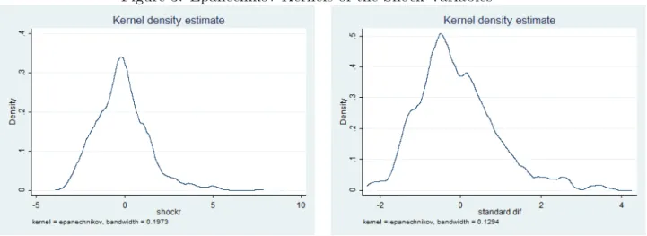
Kernels for the shock variables are available in the appendix. The rain variables are de-meaned (zi,t−z¯i, graph on the left) and standardised (on the right) and show an approximate

(23)

5 Implementation and Results

5.1 Checking the validity of the RDD assumptions

Given the data set as described previously, here are a set of comparisons between control and treated groups. In the appendix are the graphs of the covariates.

The first step for internal validity of the estimate is to check whether the running variable (the number of votes, which assigns treatment or control to the subject), is continuous. If it is, then the only discontinuity being provided by the running variable is that of allocating seemingly parties (in the number of votes) different treatments.

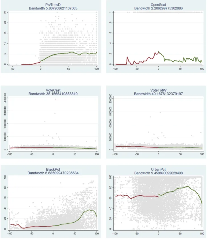
I perform the McCrary test, following from McCrary (2008). It tests whether there is discontinuity in the density of the running variable around the cutoff. In this case, whether the margin of victory’s (proportion of votes by that party minus the proportion of votes of the closest opponent) density is continuous. The test is conducted on the main 1942-2004 sample, and the smaller 1946-1996 one, and are also presented in the appendix (A.3). In both cases, I do not reject continuity of the running variable (Democratic margin of victory). The next step is to check whether there are other sources of discontinuities. To be able to identify δ, β, we must have that the only source of discontinuity is that of the discontinuous change of control to treatment, when the margin of victory running variable crosses the threshold of 0.

To do so, I test whether other variables (covariates) which could explain votes for the incumbent show discontinuities. The tests are shown in Appendix A.3. The main graphs are shown in Figure 4.6 _{The covariates include the proportion of urban and black people}

in the population of the district, previous experience of the incumbent party, among others. Others covariates have the same results, but are omitted. It is also shown that the effects of a win in t−1 seem to have no effect on the results at t, as shown by the approximately

logistic and continuous approximation of Previous Democratic Win (DWinPrv) on current Democratic Win (DemWin), in Figure 5. The same continuous effect is shown to happen in terms of Democratic Donations (DDonaPct) and Democratic Spending in that campaign (DSpndPct). Some of these are the same as in Lee (2008), but as this databse is extended it includes further covariates.

However, there is a clear discontinuity when we use the quantity of votes in the next election (t + 1) in that Congressional district (DPctNxt) with the cutoff of having won the election in (t), see figure 5 (top right-hand corner). This discontinuity is statistically significant at 10%, 5% and 1% significance levels.

6_{Regressions to test whether there is discontinuity were conducted, and the estimate for the discontinuity}

(24)

Hence, it seems that the hypotheses stated for the appropriate use of the regression discontinuity design are satisfied.

5.2 Results

All Tables are found in Appendix A.5.

The timing of shocks considered is the average for September before the reelection. This means that si,t is defined from the rainfall of the month before the reelection. This choice

considers a few factors: the shock must be not only exogenous, but should affect the district in an unavoidable manner. If enough time is given for the shock, it can be smoothed by the politician’s actions, further revenue can be transferred from federal and state resources, among many other characteristics which would distort the test which is conducted. All of this would allow for politician types (more politically able, for example) to differentiate among themselves; and the replacement would not come from the shock only. In the Robustness section, different timings are checked and the results are then discussed.

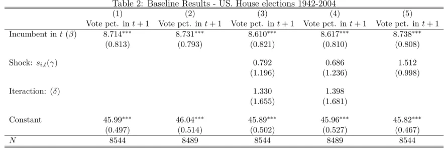
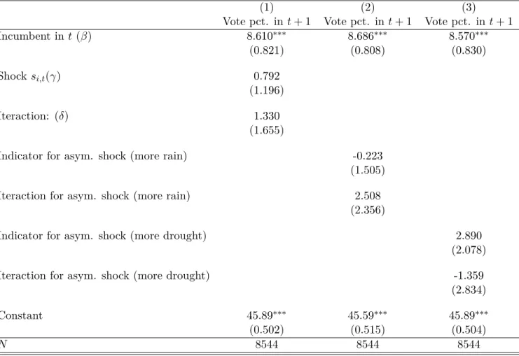
Table 1 shows the initial specifications. As expected, it seems that there is no effect of the shock upon reelections at large.

Table 2 contains the baseline results. In columns (1) and (3), the full database of 1942-2004 elections are used. In columns (2) and (4), the smaller database of 1946-1996 is used to check for any qualitative differences to the work of Lee (2008). Columns (1)-(2) show the basic incumbency regression of a RDD design, while (3)-(4) show the results of the main regression and identification of this work: equation (4).7

The results show that there is not a statistically significant effect of shocks on the incum-bent. Extreme events, i.e. negative shocks which affect revenue and economic conditions in the district, but which are observable, have lead to harm to the incumbent (since ˆδ < 0), while not to the opponent.

A realisation of a negative shock (extreme event) does not alter the incumbent’s vote. Meanwhile, it does not affect the opponent (statistically insigificant estimate). This means that there is no heterogeneity of economic shocks upon who is incumbent and who isn’t. In particular, if there was one, it would be understood as a deciding factor for many close elections.

7

Recall that the identiﬁcation is based upon equation (4).

(25)

A next step in the investigation would be to see how extreme an event must a shock be to affect the election. As discussed, it would seem that small changes in rainfall would do little to change the outcome of an election: their marginal impact would be too small, even if we disregard any measurement error.

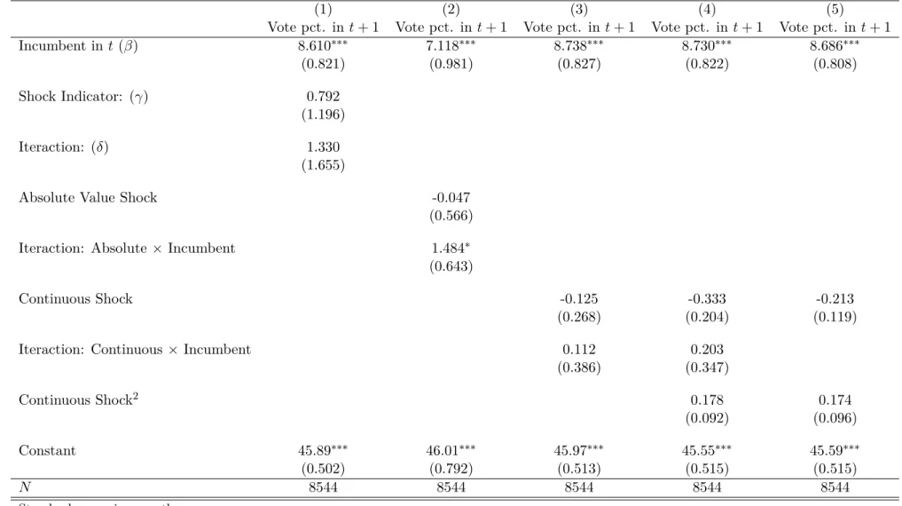
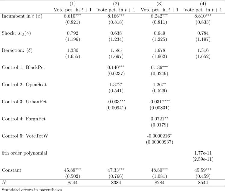
Table 3, which compares the two “shock” variables (continuous version versus indicator function for extreme vents). When a continuous variable is used, the magnitude of the effects are of a much smaller order. Column (1) is the baseline result. In column (2) of Table 2, it can be seen that the effect (γ+δ) is now smaller, and still insignificant.

As for the continous case, the test for γ+δ cannot reject that the effect is equal to zero. In essence, a small deviation of rainfall (for example, 1m.m. more in the September of the (re)election does not affect the outcomes) if you impose that rain is more damaging than drought. The positive result in one specification provides a different result than expected. It would mean the incumbent actually benefits from adverse scenarios outside his control. This does not seem to be in line with economic theory, perhaps relying on psychological explanations (such as sympathy). This is left as a discussion for future research.

An intuition can be thought as follows. When the variable is continuous, it was always unlikely that smaller changes from the historical mean could have that same effect. In reality, we would only expect that large deviations from the mean should significantly impact percentage of votes (this is captured in the baseline). Meanwhile, the continuous version incorporates both the (probably) negligible effects of small changes from the mean, with the large ones from extreme events.

This interpretation follows from δ being the marginal effect on the incumbent from changes in the variables. The final column in that table shows that small changes in rainfall, by itself, do not alter electoral results. This seems to be in line with what is expected.

A further consideration could be that what is defined as shock: extreme events in rainfall (proxying effects on the underlying economic scenario) could be asymmetric. Droughts and extreme occurrences of rainfall could possibly be asymmetric. Table 4 discusses asymmetric rain shocks (i.e. indicator now only for either 1 s.d. above the historical mean, or below, but not both). This means that we check whether extreme drought is a shock asymetrically different than extreme rainfall.

Column (1) is the baseline. Column (2) reproduces the baseline with asymmetrics for positive shocks (3) both in level (γ) and in the iteraction term forδ. Column (3) does it for negative asymmetry.

(26)

6 Results Discussions

Having Tables 1-3 in particular in mind, it is important to understand what these results seem to be pointing to.

There doesn’t seem to be a statistically significant effect of these shocks upon the votes obtained in the following election (and hence, upon reelection), and that seems to be robust to specification, controls and estimation procedure This indicates that there is no asymmetry in how exogenous, albeit observable circumstances affect elections: the incumbent seems to be favoured by a given “incumbency effect” - for example due to media exposure, but can theoretically also due to activities outside of his direct control, which might affect the economy. However, if these outside of the control factors are observable, the citizens would simply acknowledge them (as the shock is close enough that his reaction can’t be evaluated). In the theoretical model which will be shown, this is understandable: an observable shock is already incorporated by the voters. The empirical findings of Table 1 seem to point towards this direction. If it was not observable, the one in office not only has more resources, but has more information and can decide his moves. Since the politician can choose public goods provision in the model, he mayactpreemptively or incorporate any expectations of the elections to come upon his choices in office. This asymmetric choice and movement from the incumbent cannot be done by opponents, who simply campaign (i.e. cannot endogenously affect expectations by the citizens).

Larger shocks mean that, for more realisations of rainfall (ǫ in the model), the politician crosses the cutoff of it being better for him to be replaced/reelected. Recall that his decision of whether to provide public goods depends upon (ǫ) and how much that affects his own consumption. In Table 2, we see that when we use a continuous form of this shock, the magnitude is smaller. Finally, Table 3 points towards (no) asymmetry of the nature of the shocks themselves.

(27)

7 Robustness

In the appendix A.5, robustness tests are conducted forβ andδ. Tables 5 to 7 estimate them in many ways (with higher order polynomials, bandwidth optimality) and with a variety of specifications. There are no qualitative (and mostly no quantitative) differences in how they are estimated.

As discussed previously, a series of checks of whether the regression discontinuity design’s hypotheses are valid were conducted. Its results are in Appendix A.3.

In what follows, there is a discussion of how the effect varies over time (1 month before the election, with a three month average and yearly average before it). Furthermore, for robustness, shocks from after the elections are seen to not affect δ.

7.1 Variations of the effect over time

Having discussed the main econometric concerns of this estimation, as well as the robustness of the previous procedures and results, an interesting economic question can still be adressed with the data: is this significant effect which has been found, time invariant?

In other words, if this shock were to happen further away from the election, would it still have the same result? For this question, 3 month averages and yearly averages of the rainfall were calculated and estimated in the same equation as 4. This means that, instead of the shocks being those of the month before the election, they are from time frames longer than that. The results follow in Table 8.

What can be seen is that the effect seems to change over time, although not statistically. The three month average is not significant. The effect dissipates in a short period of time. From the changes in the values of the estimates, the month used is quite important.

Yearly effects follow the same idea. This means that, for a long enough time frame, unexpected shocks are not explanatory. In fact, they might be used by the incumbent and the opponent to gain votes. This follows the intuitive idea that, with a large enough time frame, more able politicians can reverse negative effects, and able opposition can explore any reaction. Some of the channels could follow Brollo et al. (2013), and that there would be political selection and better types benefit. Within the framework analysed, it would mean that the politician can reoptimise, smooth the shock and still provide the public goods for reelection.

(28)

7.2 Further tests

Table 9 presents estimates using other robustness measures. A variable called uniform is generated from randomly drawn numbers from a uniform distribution. This is used to test whether the explanations come quite simply from a sequence of shocks. This does not appear to be the case.

Another robustness conducted is to check whether shocks which happen after the elections can explain in part the effect. The idea behind this test is to check whether there could be a common factor on both shocks and votes, which explains both. In terms of the timing, it would be expected that January (if exogenous) occurrences would not affect what happened in November. Hence, by substituting January averages, of the year following the reelection as shocks, we would be checking whether they can indeed be argued as exogenous (i.e. there are no expectations which are incorporated in October or November) and whether there is a common variable to both (i.e. no time-invariant variable to both is explaining the effect). Table 9 shows that, indeed, shocks after the elections are insignificant (the joint effect γ +δ is statistically 0, with p−value > 0.1)8_{. Thus, there seems to be evidence that the}

(29)

8 Theoretical Framework

The model follows the tradition of Barro (1973) and Ferejohn (1986), who were the first to apply models of incentives to politics. In what follows, I extend the model of political agency in Persson and Tabellini (2000).9 _{The intuition is the same: an official seeks reelection, and}

the way to do so is to provide public goods. He does not gain utility from providing it, except that it gains approval by the population, which might choose to keep him in office. Voting and reelection functions as

In this model, there are many citizens, whose preferences are defined over consumption bundles and public goods, and are ex-ante identical. For these reasons, they can be inter-preted as a representive citizen. At each period, they receive an endowment w. They are free to bring their future endowment to any period, without any cost. Their intertemporal discount rate is β ∈ (0,1). Their utility function is given by U(c, g) : R2 → R, separable

in consumption and public goods, meaning U(c, g) = u(c) +h(g), and satisfies the stan-dard assumptions: both u, h are increasing, twice continuously differentiable, and satisfy u′_{(0) =}_h′_{(0) =}_∞_and _{u(c) =}_{h(g) =} _{−∞ ∀}_{c, g <}_0.

The consumer has a minimum amount of public goods that he must consume/can opt to have, ¯g, which generates utility h(¯g). This can always be achieved by the consumer if there is displacement: it is an outside option of public goods.10 _{Further assume that ¯}_{g < τ ω,}

meaning it is feasible.

There areN ≥2 politicians. They are rent-seeking, and obtain utility only from their own consumption and are ex-ante identical. Their utility function satisfies the same assumptions as above, with it being represented byv(χ). Furthermore, assumev(0) = 0, and to guarantee positive consumption,v(χ) = −∞, χ <0. Their discount rate isρ∈(0,1). There is a tax on

the consumers’ endowments to finance public goods and their private consumption. However, they cannot bring future expected revenue to t= 1, since they might not be in power then. In that sense, there is a problem of commitment which is hereby represented by separate restrictions for each period.

Public goods can be provided at a one-to-one production from the consumption goods. Tax rates are fixed, but revenue can be interpreted as stochastic (see below).

What is decribed here uses some of the evidence on the tradeoff between public goods and embezzlement, which has been described previously. The good behaviour assumed for the preferences allows the focus to be drawn on the inherent difficulties of the consumers’

9

Besley (2007) provides an overview of these models.

10_{Interpret this as the minimum of public goods which must be oﬀered so that he elects to vote or to live}

there. We can think ofh(g) =−M, M ∈R++ andh′(g) =−∞ ∀g <¯gsuﬃciently large. This assumption,

(30)

decisions under incomplete information.

There are two periods: t= 1,2. In the beginning of time, there is an incumbent (randomly chosen from the set of politicians). At the end of period 1, he will face a randomly chosen opponent from that same group.

In each period, although the citizens know their own endowment and how much they are taxed, there is uncertainty about overall (state) revenue. This is represented as an additive shock, in each period, ǫ - iid., with a positive density defined on (−τ ω,∞). There is no

impact upon the consumer’s choice, since he receives his endowment and is taxed by known amounts.

However, the overall revenue in which the politician chooses his consumption and public goods is affected. This shock is in monetary terms of each period: i.e., it has a value of 1 in t = 1 and p in t = 2, where p is the price of consumption goods in period 2, with the price in period 1 having been normalised to 1. One way to understand this is that the politician’s function of public goods provision is stochastic, with f(x) = x+ε11 _{There is a linear tax}

rate on endowment, τ. For simplicity, this tax rate cannot be readjusted.12

The timing is as follows: The consumers then go on to choose their consumption bundles. However, since they choose relative to a budget set including future endowments, they must choose in an intertemporal manner. Simulateneously, the politician chooses his own con-sumption and the provision of public goods, given the stochastic realisation of the revenue, which only he knows. Knowing the amount of public goods and, hence, their own utility, the citizens choose whether to replace the politician or not.

If he is replaced, consumers must pay a fixed costκ >0 at the goods’ price int= 1. This can be interpreted as the fixed costs of organising new elections, dissolving the government and of the work that has to be put in when a new official is chosen (new workers, changes in organizational structure and so forth). When there is displacement, the consumers pay κ off their consumer goods and get their outside option of public goods ¯g. In Appendix A.2., this is shown to be equivalent as imagining that the citizen moves to a neighbouring city: he consumes the public goods elsewhere, and faces a cost of relocation.

If there is displacement, in the following period, the consumers receive the public goods offered by the new replacement. The displaced politician receives χ2 = 0. If he remains,

consumers and the incumbent trivially choose their consumption and public goods on offer. The calculation to decide whether there is replacement is at the end of the first period: 11

This can also be thought of as a stochastic cost of monitoring the payment of taxes, the diﬃculty of accounting for all payments and so forth. Another way to see this is as if there is uncertainty about the measure of consumers in each period.

12_{This can be thought of as a congressional diﬃculty, a freeze in the budget or some other diﬃculty in}

(31)

public goods fort = 1 as well as consumption for each agent has been realised. However, he must compare what he has received to what he would have wanted. One opts for replacement if his utility with substitution is larger than what he received under the incumbent.

The consumer’s problem in the first period is, given τ, ω, and expecting g1, g2 under

beliefs µof what he expects χ1 has been, having observedg1.:

max

c1,c2 E

µ_{_U_(c

1, g1) +βU(c2, g2)} (5)

s.t.

c1+pc2 ≤ (ω+pω)(1−τ)

ci ≥ 0

where U(ci, gi) = u(ci) +h(gi)

The budget set is valid for every realisation of the shocks: those do not affect the con-sumer’s decision directly, since they know how much they can spend. The uncertainty is about overall revenue available in the economy. Notice that the decisions in periodt= 2 are trivial: having consumed c1 and chosing whether to keep the incumbent, t = 2 only yields

the consumption of c2 which follows from the equality of the budget set.

In other words, having realised the consumption c1, he will then consume c2 = 1/p((ω+

pω)(1−τ)−c1). In t= 2, he has already received g1 and receivesg2, which are not chosen

by him and, hence, do not affect his choices of c1, c2.

The politician’s problem is, given τ, ω and the revenue realised:

max

χ1,χ2,g1,g2v(χ1) +ρE

ǫ_{_v(χ

2)} (6)

s.t.

χ1 +g1 ≤ τ ω+ǫ1

χ2 ≤ I[reelected](τ ω+ǫ2−g2)

χt ≥ 0, gt ≥0, t= 1,2

Notice the decision to replace depends only on what happens in periodt = 1. The voters observe the provision of public goods and what is their utility, and then decide whether it is worth keeping the incumbent. For technical reasons, this is a good simplification, as well as it seems intuitive with regards to typical voters’ decisions.

(32)

consumption {c1, c2, χ1, χ2, g1, g2}, beliefs µ and a choice of replacement or not, such that:

• Given µ and the choice of replacement, (c1, c2, χ1, χ2, g1, g2) solve the Politician’s and

the Consumer’s problems.

• Given (c1, c2, χ1, χ2, g1, g2) and µ; the choice of replacement is such that there is

re-placement if and only if u(c1−κ) +h(¯g)> u(c1) +h(g1)

• µ is the belief a consumer has about χ1, given his observation of g1. It is consistent

and is updated through Bayes’ rule whenever possible. The Case with Observable Shocks:

Before pressing ahead, let us consider the case of complete information. Namely, that ǫ is observed by both the citizens and the incumbent.

Notice that in the case when ǫ is observed by all, there should be no replacement. The citizens can simply offer a fixed contractχ∗

1(ǫ) = ¯χ1−ǫ1, which has a fixed value ¯χsuch that

the official is not displaced, and compensates for shocks; as in Persson and Tabellini (2000). This means that, if it observable, the citizens will simply change the utility of the politician. In other words, they keep the reservation utility, u(c1 −κ) +h(¯g) and the politician is

kept in office. As will be seen further ahead, in Lemma 3, this leads to an important value of public goods which would always be provided in this case (although not when there is incomplete information). The intuition behind this case is that, since the state of nature can be observed, I can instead make a state-contingent contract, beneficial to the incumbent and to the population.13

For the rest of this model, the case in which ǫ is observable only by the politician is focused.

The Case with Unobservable Shocks:

Lemma 1. There will be replacement in a PBE iff u(c1−κ) +h(¯g)> u(c1) +h(g1).

Proof. See appendix.

The selection of this type of equilibrium regards the design of the model: a dynamic model, with uncertainty. Although there is no uncertainty regarding a “politician type”, which would require beliefs on this by the citizens; as Fudenberg and Tirole (1991) discusses, we can think of any incomplete information model as one of uncertainty on types: it is nature’s move, here, which generatesǫ1, ǫ2 and the non-observation of χmeans citizens must

infer what they are. This decision rule focuses on

13_{Assume that he is patient enough (i.e. (8), in p.40 is valid), so that he opts to consume in the next}

(33)

Corollary 1. There is no replacement if g1 ≥g¯.

Recall that period 2 is of little interest: decisions of g2 do not affect future choices,

choices of c2 and χ2 simply follow from the budget sets andthere is no futher choices of

keeping/replacing the politician. 14

The corollary means that it is always sufficient for the incumbent to provide ¯g. In fact, with a good enough realisation ofǫ1, it will be relatively less costly for him to remain. In fact,

this choice of public good provision depends crucially on the economic shock: if there are not enough funds for ¯g, he cannot “guarantee” his permanence. Naturally, in equilibrium, he will never provide above that critical value. However, notice that a provision of less than ¯

g does not mean he will be replaced.

In fact, as we will see below, there can be values in the set (0,g) where he remains.¯ Lemma 2. For κ >0small enough, there exists ag1 ∈(0,g)¯ that satisfies u(c1−κ)+h(¯g)>

u(c1) +h(g1).

When there is a fixed cost of replacement, the incumbent can afford to give a little less public goods than what is wished for. This small decrease (g1 < ¯g) is such that it is still

smaller than the cost associated with replacing him. Intuitively, it means that the citizens would accept less than desired policies as it would be too costly to change it: providing incentives, in this case, would hurt the citizens more than allowing a deviation.

Since we know that the functions are continuous, it means that there is an optimal value of g, called ˜g which is the minimum the politician must provide the population so that he remains. It suffices to simply think of diminishing g away from ¯g as long as it does not pass the inherent cost due to κ. If you continue to lower g, you will reach and pass a minimum value which equals the costs and, then, he will be replaced.

Lemma 3. For each consumption choice, in particular for the optimal ones, there exists a ˜

g1 such that u(c1−κ) +h(¯g) = u(c1) +h( ˜g1)

Now ˜g1 is called as the value of g1 which results in the equality of the decision rule for

the optimal consumption choices by the (representative) citizen.

14_{This is another simplifying assumption, for making a stylised model. However, with an inﬁnitely repeated}

(34)

Corollary 2. Given optimal consumption choices, for any g1 <g˜1 there is replacement.15

Lemma 4. In any Perfect Bayesian equilibrium, g2 = 0.

Proposition 8.1. There exists a Perfect Bayesian equilibrium, with an outcome of replace-ment occurring with positive probability.

The model is similar to a classical moral hazard problem. Punishment is dealt to the agent (politician) even if a bad outcome is not due to his effort’s selection (in this case, the budget set does not depend on his choice). The reason for that is to provide incentives: the principal (citizens) are committed to guaranteeing incentives for the provision of public goods. If the politician knew he would not be displaced, or that certainly he would, there would be no incentives to provide g1 >0 in any scenario.

However, the threat of removal guarantees that there might beg1 >0. Out of equilibrium,

when there is a good realisation ofǫ, the incumbent realises that it would be better to remain in t = 2, although not consuming in t = 1 as much. The concavity of v(·) means he would

rather transfer some of the resources for consumption in the future. That can only happen by investing in g, guaranteeing reelection and positive consumption in the next period. If he knew that he would be there in t= 2, why would he use some of the income ing?

Below, some comparative statics and discussions of the model are provided. Proposition 8.2. Comparative Statics

κ : When the fixed cost κ → ∞, there is no replacement. When κ→ 0, there are more realisations of replacement, though it does not mean that it happens always.

When there are higher occurrences of ǫ1:

g : There are no changes to g2 and no changes almost always to g1 (except on one

point, where there is positive change).

c : There are no changes in consumption (c1 and c2).

U :The value function of the consumer is non-decreasing with higher ǫ1.

χ : The private consumption χt rises with higher contemporaneous shocks (ǫt), but does

not change with (ǫj, j 6=t)

(35)

Notice that the results are incredibly similar to those by Caselli and Michaels (2013). In fact, public goods provision might rise in positive economic circumstances16_{, but less}

than what is socially best (a one-to-one rise which is the marginal rate of transformation). In fact, once there is reasonable certainty of reelection, there is little incentive to provide further public goods in the model. Meanwhile, in their work they state: “Our finding that oil windfalls translate into little improvement in the provision of public goods or the population’s living standards raises an important question: where are the oil revenues going? The natural inference is embezzlement”. This is exactly what happens in the model.

This model is able to address Caselli and Michaels (2013)’s findings, as well as those of Brollo et al. (2013) that find that an increase in transfers leads to more corruption (in the model, a relaxation of the politician’s budget set when he is not replaced leads to an increase in their private consumption due tov′_(.)_>_{0). Naturally, it seems that an apparently simple} model is rich enough to explain quite a lot of empirical evidence.

Proposition 8.3. (Adapted Average Treatment Effect) Let δˆbe defined as how changes in ǫ1 affect reelection.17

Then there exists a region in which δ >ˆ 0. Proof. See appendix A.1.

Proposition 8.4. (Comparison with no Uncertainty Benchmark) Consider the case in which there is no uncertainty (i.e. ǫt= 018 ∀t). Hence, δˆ= 0. For ρ sufficiently high, there is no

replacement of politicians in equilibirum. In all other cases, there is always replacement. Proof. See appendix A.1.

All of the dynamics in the model come simply from the misinformation the citizens face: why is the amount of public goods as such?, and is it that low because the politician is consuming too much?. In proposition 8.4, when remove the uncertainty, we are left with two trivial cases: either the politician does not want to be reelected (small ρ) or always want to do so (high ρ). Without uncertainty, it is completely in the politician’s control what can happen or not - instead of the previous decision which relies on the realization of ǫ so that he then chooses what to do, even if he is worse off (i.e. might have wanted to be reelected, but given ǫ1, chooses not to).

16_{Just on the cusp of it being advantageous to the politician to make that eﬀort to be elected, see proof}

of 8.1 in the Appendix A.1.

17_{Since all individuals are ex-ante equal, this variable Votes is discrete and assumes value of 1 if}_g _≥_g;_˜

and 0 otherwise.

(36)

Recall that this is not the same as the case in which there is uncertainty, but complete information. With complete information, citizens can simply provide a contract which neu-tralizes the effect of the shock. Here, it becomes simply a choice for the politician depending on his primitives.

The model does not need the heterogeneity of the politicians, as in Brollo et al. (2013). With heterogeneity, the citizens would have to anticipate both the type of the politician and the economic scenario. By shutting down the heterogeneity channel, the model is able to focus on the effects of ǫ, through the incentives problem, on reelection. Here, again, only the out of equilibrium events of anticipating whether it is the state of the economy or the politician’s choices which have led to poor provision of public goods is the only anticipation by the citizens. In Proposition 8.3, we see that it is enough to generate replacement.

(37)

9 Conclusion

In this work, I proposed a theoretical model which showed that politicians may be displaced from office due to adverse and unobservable economic scenarios. The model relied on the misinformation by the citizens, who cannot observe whether the public goods provision is low due to embezzlement or due to a worsening of circumstances. Hence, the removal of the incumbent works as a device to ensure their effort - since they wish to be reelected - off the equilibrium. Yet, depending upon the realisation of the state of nature, the situation might be such that they are uncapable of providing the minimum that is needed to remain in power. If, however, the shock was observable, then it should have no effect upon the chance of reelection.

The empirical approach shows evidence that this effect may happen. Using a regression discontinuity design on U.S. House Elections and taking extreme natural events as affecting the economic environment faced by the population, empirical evidence points that observable extreme events have little effect upon political outcomes, though that may vary with the time in which shocks are considered.

In a developing country, it is likely that these variables impact more electoral results. Less consolidated electoral institutions, weaker punishments for corruption and a less informed electorate could all push the results from the RDD and from the model to a stronger result. Furthermore, more precise data on shocks as well as attempts to measure more unobservable (before the elections) shocks would be possible research paths to work on.

(38)

References

Acemoglu, D. and J. A. Robinson (2001). A theory of political transitions. American Economic Review 91(4), 938–963. 12

Barro, R. J. (1973). The control of politicians: an economic model. Public choice 14(1), 19–42. 14, 29

Besley, T. (2007). Principled Agents?: The Political Economy of Good Government. Oxford University Press. 29

Besley, T. and A. Case (1995). Incumbent behavior: Vote-seeking, tax-setting, and yardstick competition. The American Economic Review, 25–45. 44

Brückner, M., A. Ciccone, and A. Tesei (2012). Oil price shocks, income, and democracy. The Review of Economics and Statistics 94(2), 389–399. 12

Brollo, F., T. Nannicini, R. Perotti, and G. Tabellini (2013). The political resource curse. American Economic Review, forthcoming. 12, 13, 27, 35, 36

Brollo, F. and U. Troiano (2012). What happens when a woman wins a close election? evidence from brazil. Working Paper, 1–37. 19

Bruckner, M. and A. Ciccone (2011). Rain and the democratic window of opportunity. Econometrica 79(3), 923–947. 11, 12, 20, 22

Caselli, F. and G. Michaels (2013). Do oil windfalls improve living standards? evidence from brazil. American Economic Journal: Applied Economics. 12, 35

Caselli, F. and A. Tesei (2011). Resource windfalls, political regimes, and political stability. CEP Discussion Papers dp1091, Centre for Economic Performance, LSE. 12, 13

Caughey, D. and J. Sekhon (2011). Elections and the regression-discontinuity design: Lessons from close u.s. house races, 1942-2008. Political Analysis 19(4), 385–408. 20

Ciccone, A. (2013). Economic shocks and civil conflict: A comment. American Economic Journal: Applied Economics. 11, 22

Cox, G. W. and J. N. Katz (1996). Why did the incumbency advantage in u.s. house elections grow? American Journal of Political Science 40(2), pp. 478–497. 9, 13, 16