E
NVIRONMENTAL
P
ROTECTION
A
ND
E
CONOMIC
G
ROWTH
V
LADIMIRK
ÜHLT
ELESR
ONALDOA. A
RRAESAgosto
de 2009
T
T
e
e
x
x
t
t
o
o
s
s
p
p
a
a
r
r
a
a
D
TEXTO PARA DISCUSSÃO 194 • AGOSTO DE 2009 • 1
Os artigos dos Textos para Discussão da Escola de Economia de São Paulo da Fundação Getulio
Vargas são de inteira responsabilidade dos autores e não refletem necessariamente a opinião da
FGV-EESP. É permitida a reprodução total ou parcial dos artigos, desde que creditada a fonte.
Escola de Economia de São Paulo da Fundação Getulio Vargas FGV-EESP
Environmental Protection and Economic Growth
Vladimir K¨uhl Teles
Getulio Vargas Foundation
Sao Paulo School of Economics
∗[email protected]
Ronaldo A. Arraes
Federal University of Ceara
Department of Applied Economics
†[email protected]
August 19, 2009
Abstract
This paper explores the link between environmental policy and economic growth by employing an extension of the AK Growth Model. We include a state equation for renewable natural resources. We assume that the change in envi-ronmental regulations induces costs and that economic agents also derive some utility from capital stock accumulationvis-`a-visthe environment. Using the Hopf bifurcation theorem, we show that cyclical environmental policy strategies are optimal, providing theoretical support for the Environmental Kuznets Curve.
Key-Words:AK Growth Model, Environmental Kuznets Curve, Hopf Bifur-cation Theorem, Limit Cycles.
JEL Class:C61, C62, D62.
∗Getulio Vragas Foundation, Sao Paulo School of Economics (EESP-FGV), Rua Itapeva, 474, 12o.
andar, 01332-000, Sao Paulo-SP, Brazil
†Universidade Federal do Ceara, Curso de P´os-Graduac¸˜ao em Economia (CAEN-UFC), Av. da
1
Introduction
The empirical evidence of Grossman and Krueger (1995, 1996), which suggests a re-lationship between per capita GNP and the emission of pollutants in the form of an inverted U, has generated great interest regarding the relationship between economic growth and environmental protection. This inverted U has been dubbed the environ-mental Kuznets curve (EKC). The issue raised by such a stylized fact is: does eco-nomic growth in itself ensure the automatic protection of the environment?
The above question has been answered positively by those who argue that a growth policy is always the best course of action. In this sense, Jorgenson and Wilcoxen (1990) have provided estimates for environmental regulation fees associated with the accumulation of capital and growth. They then verified that, during the 1974-1985 pe-riod, these costs reduced average annual growth in the U.S. by 0.2 percentage points. These results corroborate those obtained by Hazilla and Kopp (1990). At the same time, Schmalensee (1994) and Jaffe et al. (1995) have also suggested that these costs have been underestimated, since environmental regulation costs can have negative ef-fects on production rates, investment, and productivity.
The above assertions have been refuted by several studies (e.g. El Serafy and Good-land (1996), and Clark (1996)) that argue economic growth behaves indiscriminately with regard to environmental protection. The authors of these studies have insisted on the need for direct governmental intervention by taxing the use of natural resources in order to protect the environment. In support of this hypothesis, Margulis (1992) uses data from Mexico to show empirically that pollution causes serious damage to labor productivity, while Pearce and Warford (1993) have produced a detailed accounting of productivity losses from pollution in many countries.
In this paper, we investigate the EKC using an AK growth model. Some papers have included pollution in various AK models1 (e.g. Michel and Rotillon, 1995,
Mo-htadi, 1996, Smulders and Gradus, 1996, Xepapadeas, 1997, Rubio and Aznar, 2000, Reis, 2001, and Chev´e, 2002), but here we include government environmental regu-lation and the costs associated with changing that reguregu-lation. Our extensions offer a greater likelihood of understanding the empirical facts, and in particular the pollution-income relationship that underlies the EKC. In other words, we develop an AK model that predicts relevant EKC behavior.
Many papers have described the reasons for EKC using growth models (e.g. John and Pecchenino, 1994; Selden and Song, 1995; Stokey, 1996; Beltratti, 1996; Jaeger, 1998; Jones and Manuelli, 2001; Andreoni and Levinson, 2001 and Levinson, 2002). Our model, however, yields very different predictions. While most of the existing mod-els corroborate the idea that economic growth itself ensures the automatic protection of the environment, we identify a very long-term cycle between environment and income that mirrors an EKC initially, but follows an explosively different path thereafter.
1
We note from this discussion that the environmental Kuznets curve is frequently used to suggest that there is no need to tax the use of natural resources, since the growth process itself should automatically generate environmental protection. Therefore, the aim of this study is to suggest an alternative interpretation for the Kuznets curve by formalizing a growth model in which the source of the relation between growth and the environment in the inverted U format is given by the environmental regulation system itself. Under this framework, the environmental Kuznets curve is obtained from the cyclical relation that exists between environmental regulation and the long-run accumulation of capital resulting from the existence of regulatory policy adjustment costs and the insertion of a utility gain hypothesis in capital stock accumulation vis-`a-visthe environment.
In this context, we seek to make the model more realistic by relaxing the hypothesis according to which variables such as the accumulation of capital and institutional en-vironmental protection norms adjust themselves instantaneously over time. Relaxing this hypothesis abandons the theoretical simplification that makes the traditional model analytically convenient, and also offers a reasonable explanation for the environmental Kuznets curve.
The analysis developed here is divided into two parts. The first part is comprised of an extension of the AK model that takes into account the environment and the reg-ulating agent. In this regard, the relation between capital stock and the environment remains linear over time. The second part of the analysis involves the insertion of regu-latory policy adjustment costs, which results in a cyclical relation between growth and the environment, thus leading to behavior similar to the empirical findings regarding the environmental Kuznets curve.
2
Incorporating the Environment into the AK Growth
Model
The first model includes the state equation for the environment within the AK model, and assumes an overall formulation of environmental dynamics that is given by:
˙
˙
K =AK−C−R−δK (2) whereK˙ is the physical capital stock variation, Ais the productivity of the econ-omy’s various factors (where production is an AK function),C is consumption over time t, and δ is the depreciation rate. All the variables are expressed in per capita terms.
At the same time, defining the following relations,
k = (K/E) (3)
c= (C/E) (4) and
r = (R/E) (5) equations (1) and (2) may be synthesized as follows:
˙
k=k[A−δ−βr−φ+ϕk]−c−r (6) Lastly, considering that the utility of the agents depends on the relationships be-tween consumption and the environment, and bebe-tween the rate of regulation and the environment, we derive the following intertemporal optimization problem for the so-cial planner:
max
∞
R
0
e−ρt
u(c, r)dt
s.t. k˙ =k[A−δ−βr−φ+ϕk]−c−r
(7)
where ρ > 0 is the temporal discount rate. This equation is a simple dynamics optimization model with two control variables,randc, and a state variable,k.
The current Hamiltonian value is given by,
H =u(c, r) +λ[k(A−βr−φ+ϕk)−c−r] (8) whereλis the co-state variable. The first order conditions are:
ur =λ(βk+ 1) (9)
uc =λ (10) and
˙
˙
λ λ =η
˙ r r − ˙ k k βk
(βk+ 1) (12)
whereη=rurr
ur is the elasticity of the marginal utility with respect to the regulation
rate - environment ratio, which we assume to be constant. Thus, equating (12) and (11), and using (6), we arrive at:
˙
r r =
ρ− βk1+1(A−δ−φ+ϕk+βc)−ϕk
η (13)
at the same time, rewriting (6) we have:
˙
k
k = [A−δ−βr−φ+ϕk]− c k −
r
k (14)
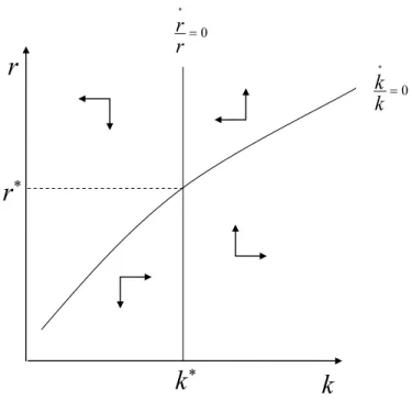
Thus, equations (13) and (14) describe the optimal trajectory of r and k. These trajectories are illustrated in Figure 1. The ( ˙r/r) = 0 function is vertical in space
k−r, since:
dr dk ¯ ¯ ¯ ¯ ¯r˙
r=0
= 0 (15)
At the same time, the shape of the( ˙k/k) = 0function in spacek−ris given by:
dr dk ¯ ¯ ¯ ¯ ¯k˙
k=0
= A−δ−φ+ 2ϕk+β(c+ϕk
2)
(1 +βk)2 (16)
This will be positive if the natural recomposition of the environment, φ, and the capital depreciation are small enough. This is an expected result given that the optimal environmental regulation tax will increase with the value of capital stock only if the natural environment cannot repair itself.
The phase diagram that illustrates the dynamics of the economy is presented in Figure 1. In that sense, ifk > k∗
, the optimal path is obtained through an increase inr, and ifk < k∗
,rmust decline in order to achieve the optimal dynamics. Accordingly, tax regulation should be used in order to maintaink at the constantk∗
level. At same time, ifris above thek/k˙ = 0isocline, given a value ofk, the capital stock will fall. And ifris below the isocline,kwill increase.
The phase diagram in Figure 1 implies an unstable solution path in a counterclock-wise spiral. So, whenkis growing,ris falling and the environment is being depleted. But, later,r may begin to rise and the growth in k falls. This trajectory is similar to that depicted in the EKC.
3
Adjustment Costs of Regulation and the
Environmen-tal Kuznets Curve
Although the analysis outlined in section 2 provides us with important hypotheses for our analysis, we can also develop the model by incorporating adjustment costs for environmental regulation policies in order to analyze the consequences on the the environmental Kuznets curve’s dynamics. This is an important advance once we better describe the choice of regulation policies given an optimal path. Also, as is made clear by the evidence presented in Grossman and Krueger (1995), it is probable that those countries that have reached the ”end” of the environmental Kuznets curve will once again manifest environmental misuse trends as per capita income increases. In other words, the relation between the environment and growth seems to display cyclical behavior in the long run.
In an attempt to provide an explanation for these facts, we suggest that there are adjustment costs in terms of both capital stocks and environmental regulation policies. In this context, relaxing the hypothesis stating that variables like the accumulation of capital and institutional environmental protection rules are instantaneously adjusted over time makes the model more realistic. It accomplishes this by abandoning a certain theoretical simplification in order to make the traditional model more analytically con-venient. Thus, the insertion of a cyclical relation between the accumulation of capital and the environment is obtained by applying the Hopf Bifurcation Theorem, following the methodology proposed by Feichtinger et al. (1994).
Therefore, we consider that the utility function of the social planner is given by
u(c, r) +v(k)−z(Φ), where u(c, r) is the function that determines how the utility varies in relation to consumption and environmental regulation. The main part of the social planner’s utility function, which is the basis for the explanation of non-linearity in the relationship between growth and the environment, is the second part, where the non-linearities are included. The functionz(Φ)symbolizes the social planner’s disu-tility and the changes in environmental regulations. There are plenty of reasons to believe that there is some rigidity in environmental regulations and that it is difficult to implement environmental tax reforms that are associated with political and eco-nomic costs (Smulders, 2004). In addition, and as explained by Wirl (1999, p.23), it is
”[o]bvious [that] scrubbers, filters, catalytic converters and other abatement devices are costly investments that take time. These costs account for the fact that the reduc-tion of pollureduc-tion, waste disposal, etc. is costly and sluggish”. Therefore, we account for the assumption that there are costs in implementing environmental regulations. At the same time, the functionv(k)seeks to include capital externalities in the problem, following Feichtinger et al. (1994).
max
∞
R
0 e
−ρt
[u(c, r) +v(k)−z(Φ)]dt s.a. k˙ =k[A−βr−φ+ϕk]−c−r
˙
r= Φ lim
t→∞e −ρt
λkk = 0 lim t→∞e
−ρt
λrr = 0
(17)
This way, the current Hamiltonian value for problem (17) is given by:
H =u(c, r) +v(k)−z(Φ) +λk[k(A−βr−φ+ϕk)−c−r] +λrΦ (18) Thus, the first order conditions are:
uc =λk (19)
zΦ =λr (20)
˙
λk =ρλk−vk−λk[A−βr−φ+ 2ϕk] (21)
˙
λr =ρλr−ur+λk(βk+ 1) (22) To simplify, we consider the utility function as being additively separable, and given byu(c, r) =ζc+ξr, the functionv(k) =v0k, and an adjustment that is costly
and quadratic, in accordance the suggestion of Wirl (2000), expressed as z(Φ) = 1/2γΦ2.
The hypothesis of an additive utility function was used to simplify our analysis. This hypothesis means that substitutability among goods does not depend on the quan-tity of that good consumed by society, and that at least one of the intertemporal substi-tution elasticities is assumed to be constant. That leads to a rigorous restriction regard-ing the social planner’s behavior. Nevertheless, the hypothesis is commonly used in the literature for simplification purposes, as in Long and Plosser (1983). In addition, conclusive evidence that annuls this hypothesis does not stand, as that additivity has been detected by Selvanathan (1987), Clements et al. (1997) and Fleissig and Whitney (2007).
Thus, by substituting (19) and (20) into (21) and (22), and by applying the specifi-cations of the functions suggested here, the canonic equations are given by:
˙
k =k[A−βr−φ+ϕk]−c−r (23)
˙
r= λr
γ (24)
˙
˙
λr =ρλr−ξ+λk(βk+ 1) (26) Therefore, the steady-state solutions obtained from the transversality conditions, and from (23) to (26), are given by:
r∗ = ³ξ −ζ ζβ ´2
(−ϕ) +³ξ−ζ
ζβ
´
(A−φ)−c
³ξ
−ζ
ζ + 1
´ (27)
k∗
=
Ã
ξ−ζ ζβ
!
(28)
λ∗
r = 0 (29)
λ∗
k =ζ (30)
Thus, in order to apply the Hopf Bifurcation Theorem, we must obtain the Jacobian of (23) through (26), whose evolution around the steady-state (27) through (30) is given by: J =
X −(βk∗
+ 1) 0 0
0 0 0 1γ
−(λ∗
kα(ϕ)) λ
∗
kβ ρ−X 0
λ∗
kβ 0 (βk
∗
+ 1) ρ
(31)
whereX = [2k∗
−βr∗
+A−φ+ 2ϕk∗
].
Also, according to Dockner and Feichtinger (1991), the eigenvalues of a Jacobian of type (25) are given by,
3
1θ42 =ρ/2±
r
(ρ/2)2−Y/2±(1/2)qY2−4 det (J) (32)
whereY is the sum of the determinants,
¯ ¯ ¯ ¯ ¯ X 0
−(λ∗
kα(ϕ)) ρ−X
¯ ¯ ¯ ¯ ¯ + ¯ ¯ ¯ ¯ ¯
0 1/γ
0 ρ ¯ ¯ ¯ ¯ ¯ + 2 ¯ ¯ ¯ ¯ ¯
−(βk∗
+ 1) 0
λ∗
kβ 0
¯ ¯ ¯ ¯ ¯ (33)
However, this Jacobian has a pair of eigenvalues that are purely imaginary if, and only if, the conditions
Y2+ 2ρ2Y = 4 det (J) (34)
and
For our model, the Constant,Y, and the determinant,det(J), are given by,
Y =X(ρ−X) (36)
det (J) = 1
γ
h
(2X−ρ)λ∗
kβ(βk
∗
+ 1)−(βk∗
+ 1)2(2λ∗
k(ϕ))
i
(37)
By applying the bifurcation conditions of (34) through (36) and (37), and by choos-ingγ as a bifurcation parameter, it is then possible to find the critical valueγcrit given by:
γcrit =
h
(2X−ρ)λ∗
kβ(βk
∗
+ 1)−(βk∗
+ 1)2(2λ∗
k(ϕ))
i
X(ρ−X)
2
³X(ρ−X)
2 +ρ2
´ (38)
Note that the steady-state values for(k, r, λk, λr)do not depend on the parameter
γ. Given these results, it is possible to formulate proposition 3, as follows:
Proposition 1 Considering the optimal control problem (17) and the equilibrium
prob-lem (27)-(30), Hopf ’s bifurcation, usingγ as a bifurcation parameter (whose critical value is determined by (38)), and assuming the validity of (34) and (35), leads to a limit in cycles.
Proof: Given the choice of the other parameters of the model, and considering the
validity of conditions (34) and (35), the critical value may be calculated from (38). In such a case, the Jacobian arising around equilibrium assumes a purely imaginary pair of eigenvalues, with a non-null crossing velocity, such that it may be concluded that there are periodical solutions for bothγ > γcrit andγ < γcrit.
Our proposition establishes that the inclusion of regulatory policy adjustment costs in the AK growth model with environment, which was developed in section 2, gener-ates cyclical behavior involving a tension between the environment and the accumula-tion of capital stock. This theoretical formulaaccumula-tion provides a plausible explanaaccumula-tion for the stylized facts presented by Grossman and Krueger (1995, 1996).
The basic link between this result and the environmental Kuznets curve is the non-linear relationship between pollution and economic growth. At the beginning of the development, regulatory institutions are not well established, and economic growth is therefore accompanied by increasing pollution. When the regulatory institutions receive the opportunity to tax pollution emissions, they do so more than proportionally because they know that there are costs to changing the regulatory tax. Thus, economic growth will be accompanied by a decrease in pollution.
We did not obtain any evidence for the cycles’ stability. This is consistent with Wirl (1999), who demonstrated that the use of two state variables instead of one can increase complexity in the sense of optimum policies for environmental regulation leading to system instability. In other words, a rational strategy for an environmental policy does not necessarily imply stability (i.e., the sustainability of the environment). Lastly, the theoretical suggestion offered by this model becomes relevant because it provides a formal answer to the statement that growth itself generates environmental protection mechanisms, thus justifying the need to protect the environment. We note that this model suggests the attention given to the environmental regulation problem ends up levelling off the environmental cycle, and that the environment is thus affected to a lesser degree. This result is fundamental since there is evidence that most natural resources are not renewable, making the role of environmental protection all the more crucial.
4
Final Considerations
After the empirical evidence produced by Grossman and Krueger (1995,1996) showed that the relationship between per capita income and the concentrations of certain pol-lutants assumes an inverted-U shape, the economic literature has offered a vast array of theoretical alternatives for this fact, triggering an intense debate regarding environ-mental policies that might be adopted to address the issue.
Given this debate, our study sought to investigate the aforementioned relationship by suggesting a model for the environmental Kuznets curve. Our theoretical work is based on an expansion of the traditional AK growth model. Under our frame-work, the environmental Kuznets curve is obtained from a cyclical relation that exists between environmental regulation and the long-term accumulation of capital, which is due to the existence of regulatory policy adjustment costs and the statement of the hy-pothesis that there is a utility gain to capital stock formationvis-`a-visthe environment. In this context, we have sought to make the model more realistic by relaxing the hy-pothesis that variables like the accumulation of capital and institutional environmental protection regulations adjust instantaneously. The relaxation of this assumption aban-dons a theoretical simplification that was originally adopted to make the traditional model more analytically convenient and to offer a reasonable explanation for the envi-ronmental Kuznets curve.
traditional AK model with inclusion of the environment and a regulating agent. This is a simple introduction to the main model.
The second part of the analysis considers the inclusion of regulatory policy adjust-ment costs, and posits a cyclical relation between the environadjust-ment and growth. The resulting system behaves similarly to the empirical findings observed for the environ-mental Kuznets curve.
The results obtained here not only provide an explanation for the empirical ev-idence of a non-linear relationship between the environment and growth, but also show that this relationship may be the consequence of policies that reflect the com-plex choices associated with the adjustment costs of environmental regulation. In par-ticular, our results suggest that the optimum policy strategy may be unstable, where environmental sustainability is not optimum. This further suggests that the evidence from the Kuznets environmental curve does not contradict this prediction.
Thus, one of the conclusions of this study is the crucial emphasis on the fact that the environmental Kuznets curve, by itself, does not mean that economic growth leads automatically to environmental development. Rather, the environmental Kuznets curve is the result of a very long-term cyclical process between growth and the environment.
References
[1] ANDREONI, J. and A. LEVINSON (2001), ”The simple analytics of the envi-ronmental Kuznets curve”,Journal of Public Economics80: 269-286.
[2] BELTRATTI, A. (1996), Sustainability of Growth: Reflections on Economic Models(Kluwer Academic, Dordrecht Publishers).
[3] CHEV ´E, M. (2000), ”Irreversibility of pollution accumulation”, Environmental and Resource Economics16: 93-104.
[4] CLARK, C. W. (1996), ”Operational Environmental Policies”,Environment and Development Economics1: 110-113.
[5] CLEMENTS, K., YANG, W., ZHENG, S., (1997). Is utility additive? The case of alcohol.Applied Economics29, 1163-1167.
[6] DOCKNER, E. and FEICHTINGER, G. (1991), ”On the Optimality of Limit Cycles in Dynamic Economic Systems”,Journal of Economics53: 31-50.
[7] EL SERAFY, S. and GOODLAND, R. (1996) ”The Importance of Accurately Measuring Growth”Environment and Development Economics, 1, 116-9.
[9] FLEISSIG, A. and WHITNEY, G. (2007) Testing additive separability. Eco-nomics Letters96 p. 215-220.
[10] GROSSMAN, G. and KRUEGER, A. (1995) ”Economic Growth and the Envi-ronment”.The Quarterly Journal of Economics, v.110, n.2, May, p.353-377.
[11] GROSSMAN, G. and KRUEGER, A. (1996) ”The Inverted-U: What Does it Mean”Environment and Development Economics1, 119-122.
[12] HAZILLA, M. and KOPP, R. J. (1990) ”Social Cost of Environmental Quality Regulations: A General Equilibrium Analysis” Journal of Political Economy, 98, p. 853-73.
[13] JAEGER,W. (1998), ”Growth and environmental resources: A theoretical basis for the U-shaped environmental path”, mimeo, Williams College.
[14] JAFFE, A. B., et. al. (1995) ”Environmental Regulation and The Competitivive-ness of U.S. Manufacturing: What Does the Evidence Tell Us?”Journal of Eco-nomic Literature, 33, 132-63.
[15] JOHN, A. and R. PECCHENINO (1994), ”An overlaping generations model of growth and the environment”,The Economic Journal104: 1393-1410.
[16] JONES, L. and R. E. MANUELLI (2001), ”Endogenous policy choice: The case of pollution and growth”,Review of Economic Dynamics4: 369-405.
[17] LEVINSON, A. (2002), ”The ups and downs of the environmental Kuznets curve”, in: J. List and A. de Zeeuw, eds., Recent Advances in Environmental Economics(Edgar Elgar, Cheltenham).
[18] LONG, J.B., PLOSSER, C., 1983. Real business cycles. Journal of Political Economy91 (1), 39-69.
[19] MARGULIS, S. (1992) ”Back-of-the-Envelope Estimates of Environmental Damage Costs in Mexico” Policy Research Working Papers, The World Bank, Washington, January 1992.
[20] MICHEL P. and G. ROTILLON (1995), ”Disutility of pollution and endogeneous growth”,Environmental and Resource Economics6: 279-300.
[21] MOHTADI, H. (1996), ”Environment, growth, and optimal policy design”, Jour-nal of Public Economics63: 119-140.
[22] PEARCE, D.W. and WARFORD, J.J. (1993) A World Without End: Economics, Environment, and Sustainable Development, Oxford: Oxford University Press.
[24] RUBIO, S.J. and J. ASNAR (2000), ”Sustainable growth and environmental poli-cies”,Fondazione Eni Enrico Mattei Discussion Paper25.2000.
[25] SCHMALENSEE, R. (1994) ”The Costs of Environmental Protection” in M. KOTOWSKI (Ed.), Balancing Economic Growth and Environmental Goals, p. 55-75.
[26] SELDEN, T.M. and D. SONG (1995), ”Neoclassical growth, the J curve for abatement, and the inverted U curve for pollution”, Journal of Environmental Economics and Management29: 162-168.
[27] SELVANATHAN, S., 1987. A Monte Carlo test of preference independence. Eco-nomics Letters25, 259-261.
[28] SMULDERS, S. (2004) Economic growth, liberalization and the environment.
Encyclopedia of Energy, Cutler Cleveland (ed) Elsevier
[29] SMULDERS, S. and R. GRADUS (1996), ”Pollution abatement and longterm growth”,European Journal of Political Economy12: 505-532.
[30] STOKEY, N. (1998) ”Are There Limits to Growth?”International Economic Re-view, v.39, n.1, p.1-31.
[31] WIRL, F. (1999) Complex dynamic environmental policies.Resource and Energy Economics. 21, 19-41.
[32] WIRL, F. (2000) ”Optimal Accumulation of Pollution: Existence of Limit Cycles for The Social and The Competitive Equilibrium”Journal of Economic Dynamics and Control, 24, p.297-306.
[33] XEPAPADEAS, A. (1997), ”Economic development and environmental pollu-tion: Traps and growth”, Structural Change and Economic Dynamics 8: 327-350.
Figure 1:
* *
0
*
=
r
r
0
*
=