EVIDENCE OF THE ENVIRONMENTAL KUZNETS CURVE: IMPLICATIONS OF INDUSTRIAL TRADE DATA

ISSN: 1553-345X

©2013 Science Publication

doi:10.3844/ajessp.2013.130.141 Published Online 9 (2) 2013 (http://www.thescipub.com/ajes.toc)

Corresponding Author: Jamalludin Sulaiman, School of Social Sciences, University Sains Malaysia, Penang, Malaysia

EVIDENCE OF THE ENVIRONMENTAL KUZNETS

CURVE: IMPLICATIONS OF INDUSTRIAL TRADE DATA

Jamalludin Sulaiman, Azlinda Azman and Behnaz Saboori

School of Social Sciences, University Sains Malaysia, Penang, Malaysia

Received 2013-02-08, Revised 2013-02-21; Accepted 2013-05-10

ABSTRACT

This study examines the dynamic relationship between CO2 emissions and economic growth in Malaysia for the period of 1980-2004. The evidence of the Environmental Kuznets Curve (EKC) is tested by including energy consumption, dirty export from Malaysia to China and dirty import from China to Malaysia based on the two and three-digit ISIC data which reflect pollution-intensive manufacturing. Using dirty industries for the period of 1980-2004, the existence of Pollution Haven Hypothesis (PHH) was tested by employing ARDL approach of cointegration and the Fully Modified Ordinary Least Squares (FMOLS). Six out of eight dirty industries are found to show statistically significant inverted U-shaped relationship between CO2 emissions and economic growth, thus the EKC. Export from industries such as textile, wearing apparel and leather, manufacture of fabricated metal products and electrical machinery significantly increase CO2 emissions in Malaysia. Most of the import coefficients are significant and positively related to CO2 emissions, which is in contrast to the PHH. This strongly rejects the PHH for CO2 emissions in Malaysia-China trade. There is no evidence that domestic production of pollution-intensive goods in Malaysia is being replaced by imports from China. Based on the analysis, Malaysia-China bilateral trade increases CO2 emissions in Malaysia. There is therefore urgent need that electricity generation in Malaysia is from clean and sustainable sources. There have been efforts by the Malaysian government towards achieving this objective through its many related policies introduced since the beginning of this new millennium.

Keywords: CO2 Emissions, Energy Consumption, Malaysia-China Industrial Trade

1. INTRODUCTION

Growth and development is not without consequences, either socially, politically and especially environmentally, given the world’s limited and unevenly distributed resources. With globalization and trade made easier, growth and development can also lead to environmental problems in the economies of the trading partners. Environmental degradation often times can also lead to possible long-term debilitating consequences to the society, if not adequately and quickly addressed.

Malaysia, a relatively small country in South East Asia with about 28 million population, is probably the second leading economy after Singapore in the region. It has experienced remarkable economic growth over the past three decades made possible by effective economic structural transformation and an open trade regime

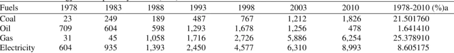
Table 1. Total energy consumption by sectors (ktoe)

Fuels 1978 1983 1988 1993 1998 2003 2010 1978-2010 (%)a

Coal 23 249 189 487 767 1,212 1,826 21.501760

Oil 709 604 598 1,293 1,678 1,256 478 1.641410

Gas 31 45 1,058 1,716 2,726 5,886 6,254 25.378910

Electricity 604 935 1,393 2,450 4,577 6,310 8,993 8.605175

Reference: Malaysia Energy Information Hub (MEIH) (http://meih.st.gov.my/). a Average annual growth rate

Malaysia experienced a significant increase in its CO2 emissions from 1460 million tons (Mt) in 1970 to 6499 Mt in 2007 World Bank, online database (www.worldbank.org). Table 1 shows that over period 1978-2010 the coutry’s dependency on oil has decreased while there is still a significant growth in coal, coke, gas and electricity consumption.

Malaysia’s main trade partners are the United States (US), Japan, Singapore and China. The percentages of export to and imports from the US, Japan and Singapore have declined in recent years, while the trade between China and Malaysia has increased considerably during past two decades.

Since the emergence of China as a major exporter of manufactured goods in 1990s, intra-regional trade among East Asian region countries has also expanded. China is the largest source of imports and the second largest export destination for Malaysia. Importantly, almost half of the bilateral trade between these two countries is in Electrical and Electronics (E and E) industries.

Bilateral trade with China in the E&E industries has risen to 47% of total Malaysian imports and 51% of total exports in 2010 (Department of Statistics Malaysia, External Trade Sta-tistics System. Electrical and electronics goods corres-ponding to the SITC, Revision 4 classification numbers 75, 76, 77 and 813). Evidence has shown that China is Malaysia’s most polluted trade partner. In the five-year period, from 2002 to 2007, China’s CO2 emissions doubled and it is now believed that China is the world’s biggest emitter of CO2 emissions. Evidently, there is an obvious need for a study to determine the environmental impacts of the Malaysia-China trade.

Unlike previous studies, this study goes beyond the existing literatures in three ways. First, previous studies examined the relationship between CO2 emissions, economic growth, energy consumption and foreign trade used trade openness as a proxy for foreign trade. Given the possible aggregation bias, this study uses detailed data on dirty trade flows between Malaysia and China. Second, this study employs a time series technique, as cross-sectional panel data analysis could be misleading because individual countries do not possess the same pollution path that is assumed in panel data analysis; and

third, one of the main interests of this research is whether Pollution Haven Hypothesis (PHH) influences the EKC functional form. PHH as will be explained later is the consequence of trade between trading partner countries with relatively lax environmental laws.

The proposed EKC model used energy consumption, dirty imports from China to Malaysia and dirty exports from Malaysia to China based on two and three-digit ISIC data reflecting pollution intensive manufacturing. The long-run effects of the mentioned variables on CO2 emissions for the period of 1980-2004 was investigated, using ARDL bounds testing approach of cointegration developed by Pesaran and Shin (1999) and Pesaran et al. (2001) and Fully Modified Ordinary Least Squares (FMOLS) proposed by Phillips and Hansen (1990).

A number of studies have examined the relationship between environmental degradation and economic growth (Grossman and Krueger, 1991; Panayotou, 1993; Selden and Song, 1994; Shafik, 1994). Central to these studies is the Environmental Kuznets Curve (EKC) hypothesis suggesting an inverted U-shaped relationship between economic growth and environmental degradation.

A main criticism of The EKC in its basic form is that it does not include trade variables (Cole, 2004), although literatures on the environmental impacts of trade are abound (Copeland and Taylor, 1994; Antweiler et al., 2001; Cole and Elliott, 2003). Grossman and Krueger (1991) decomposed the possible environmental effects of trade into three groups-scale, technique and composition effects.

A number of studies have concentrated on the relationship between the environmental pollutants and economic growth using the EKC hypothesis. Many related studies are available in Stern (2004) and Dinda (2004). More recent examples are those of Dinda and Coondoo (2006); Managi and Jena (2008); Fodha and Zaghdoud (2010); Narayan and Narayan (2010); He and Richard (2010). There are some studies that incorporate other determinants of pollution to the EKC model such as energy consumption (Ang, 2007; Soytas et al., 2007; Ozturk and Acaravci, 2010), urbanization (Zhang and Cheng, 2009; Hossain, 2011) and foreign trade (Halicioglu, 2009; Jalil and Mahmud, 2009; Nasir and Rehman, 2011) (A common concern in these studies is poor representation of trade in the analysis, as they employed openness ratio as a proxy for foreign trade).

Another group of studies focuses on the relationship between trade liberalization and pollution emissions (Anderson and Blackhurst, 1992; Esty, 1994; Chichilnisky, 1994; Copeland and Taylor, 1994; Cole, 2000; Copeland, 2005). ecifically, trade among countries with different environmental regulations makes those with stringent environmental regulation cleaner than those with fewer regulations.

A main critique on the previous studies using EKC is for not considering the movement of goods between countries that embody pollution (PHH), most significantly is an article by Suri and Chapman (1998). Cole (2004) concludes that if the PHH is correct, then excluding exports and imports of dirty industries may produce bias and inconsistent estimates of EKC and the related turning point. Stern (2004), in a critical review, establishes empirical analyses in order to relate EKC and international trade. Suri and Chapman (1998) included the ratio of manufacturing exports and imports to domestic manufacturing production as independent variables in their model, to test the existence of EKC for energy consumption.

Friedl and Getzner (2003) included import/GDP ratio in the model. Cole (2004) included trade openness, ratio of GDP in manufacturing and dirty trade flows to the model to test the EKC for ten air and water pollutants for selected OECD countries. Kearsley and Riddel (2010) extends Cole (2004) study by using disaggregated estimates of import and export shares based on two and three-digit levels for dirty industries in OECD countries. However the evidence on PHH is mixed. While (Mani and Wheeler, 1998; Cole, 2004; Kearsley and Riddel, 2010) find evidence of pollution havens, the relationship between stringency of a country’s environmental regulation and trade in dirty products is rejected by (Jaffe et al., 1995; Janickle et al., 1997).

The rest of the study is structured as follows: section 2 presents the data and model, section 3 explains the methodology, the fourth section discusses the empirical results and the last section concludes the study.

1.1. Data and Model

This study uses annual data from 1980 to 2004. The sample is chosen based on the availability of all data. Per capita CO2 Emissions (E) are measured in metric tons. Real per capita GDP (Y) is in constant 2000 US dollars. Per capita commercial energy consumption (EN) is measured as kg of oil equivalent. i

t

DM is measured as the ratio of imports from China in ISIC sector i to total imports and i

t DX is measured in the same way for exports. Four exports and imports variable corresponding to each of the four 2-digit ISIC sectors for dirty industries (31, manufacture of food, beverages and tobacco; 32, textile, wearing apparel and leather industries; 35, manufacture of chemical, petroleum, coal, rubber and plastic products and 38, manufacture of fabricated metal products, machinery and equipment) and four export and import variables corresponding to the four 3-digit ISIC codes for dirty industries (311, food products; 321, textiles; 382, machinery except electrical and 383, machinery and electrical) (These industries have been chosen based on availability of the reliable data.) were used in the study. The data for real GDP per capita and per capita energy consumption were taken from World Development Indicators (WDI). The per capita CO2 emissions data was taken from U.S. Energy Information Administration (EIA).

i t

DM and i

t

DX have been collected from the World Bank’s Trade, Production and Protection Database 2006.

Halicioglu (2009); Jalil and Mahmud (2009); Ghosh (2010) examined the relationship between CO2 emissions per capita, GDP per capita, per capita energy consumption and foreign trade. The basic model is:

2

t 0 1 t 2 t 3 t 4 t t

ln E = α + α ln Y+ α(ln Y ) + α ln EN + α ln TR + ε

Where:

E = Per capita CO2 emissions Y = represents per capita real income

EN = stands for commercial energy consumption per capita

TR = is openness ratio which is used as a proxy for foreign trade and

εt = is the standard error term (We estimate Equation (1) for four 2-digit and four 3-digit dirty industries)

emissions may offer a biased forecast of future emissions if the PHH is correct. If countries with high environmental regulation are effectively exporting waste, the EKC for these countries will give turning points that are not replicable. Pollution havens will not enjoy the environmental quality improvements as per capita income rises and current estimates of the EKCs will give overly optimistic projections of future emissions for developing countries. According to Cole (2004), omitting i

t DM and

i t

DX may bias coefficient estimates of GDP and GDP2, resulting in a biased estimates of the EKC’s turning point. Although Cole (2004) contribution is significant in that it recognizes that excluding dirty exports and imports from the EKC can bias coefficient estimates of income, he uses aggregated measures of dirty imported and export shares to predict emissions. This may be problematic if the marginal changes in emissions vary across the dirty manufacturing sectors. If this is the case, then EKC estimation based on aggregated trade data may give a false picture of the EKC relationship (Kearsley and Riddel, 2010). In the light of the above discussion, the following EKC model is used for the study:

2

t t t

i i

t t t t

ln E ln Y (ln Y )

ln EN ln DX ln DM

= α + β + δ

+ϕ + φ + γ + ε (1)

Where:

E = Per capita CO2 emissions Y = Represents per capita real GDP

EN = Stands for commercial energy use per capita

i t

DX = The ratio of dirty export to China in dirty manufacturing sector i to total export

i t

DM = The ratio of dirty imports in manufacturing sector i from China to Malaysia to total imports and εt is the standard error term

Based on EKC hypothesis the sign of βis expected to be positive whereas a negative sign is expected for δ. The turning point of per capita real income is Y* = -β1/2δ2. If the variable Y is measured in logs then exp (Y*)will yield the monetary value representing the peak of the EKC. Since a higher level of energy consumption leading to greater economic activity and stimulates CO2 emissions, φis expected to be positive. The relationship between pollution and dirty trade is considered next. If the coefficient of the share of dirty imports γ is negative, then evidence for the PHH is established. PHH refers to the possibility that multinational firms, particularly those with pollution intensive activities, relocate to countries with

lower environmental standards. Specifically developing countries produce pollution-intensive goods for developed countries’ consumption. If the coefficient of the share of dirty export (ϕ) is positive, this would validate the choice of industries indentified as pollution intensive.

2. MATERIALS AND METHODS

Testing for cointegration relationship is very important as it can assure consistent results and a long-run equilibrium relationship between variables. This study employs the Autoregressive Distributed Lag (ARDL) methodology proposed by Pesaran et al. (2001). ARDL for cointegration analysis has a number of attractive advantages over the alternatives (Pesaran and Shin, 1999). The main advantage being that it does not require establishing the order of integration of the variables (unit-root test). The approach is applicable regardless of whether the underlying regressors are I(0), I(1) or fractionally integrated while the other standard cointegration approaches such as (Engle and Granger, 1987; Johansen and Juselius, 1990) require that variables should be integrated at a unique level of integration. So the ARDL approach is free of pre-testing problems associated with the order of integration of variables. The ARDL bounds testing approach is chosen for this study to examine the cointegration relationship among CO2 emissions, economic growth, energy consumption and international trade. The ARDL framework of Equation (1) of the model is as follows:

t 0

n n n

2

1k t k 2k t k 3k t k

k 1 k 0 k 0

n n

i

4k t k 5k t k

k 0 k 0

n

i

6k t k

k 0

2

1 t 1 2 t 1 3 t 1 4 t 1

i i

5 t 1 6 t 1 t

ln E

ln E ln Y ln(Y )

ln EN ln DX

ln DM

ln E ln Y ln(Y ) ln EN

ln DM ln DX

− − −

= = =

− −

= =

− =

− − − −

− −

∆ = λ +

λ ∆ + λ ∆ + λ ∆

+ λ ∆ + λ ∆

+ λ ∆

+ψ + ψ + ψ + ψ

+ψ + ψ + ε

∑

∑

∑

∑

∑

∑

(2)

where, ∆ is the first difference operator, λ0 is drift component and εtwhite noise.

F-statistics are available in Pesaran and Pesaran (1997); Pesaran et al. (2001) (This study adopts the critical values of (2001) for the bounds F-test.). Two sets of critical values for a given significance level are available for with and without a time trend, for I(0) and I(1) known as the Lower Bounds (LCB) and Upper Bounds (UCB) critical values respectively. This then provide a band covering all possible classifications of the variables into I(0) and I(1). If the computed F-statistic is higher than the UCB the null hypothesis of no cointegration is rejected and if it is below the LCB the null hypothesis of no cointegration cannot be rejected and if it lies between the LCB and UCB the result is inconclusive. At this stage of the estimation process the unit root tests are normally carried out on variables entered in to the model (Pesaran and Pesaran, 1997). The lag order of the variables is then selected using Schawrtz-Bayesian Criteria (SBC) and Akaike’s Information Criteria (AIC). SBC selects the smallest possible lag length while AIC selects maximum relevant lag length. Once a cointegration relationship has been established, the Error Correction Model (ECM) can be estimated. A general ECM of Equation (2) is formulated as follows Equation (3):

n n

t 0 1k t-k 2k t -k

k=1 k=1

n n n

2

3k t-k 4k t-k 5k

k=1 k =1 k=1

n

i i

t-k 6k t-k t -1 t

k=1

lnE =λ + λ lnE + λ lnY

+ λ (lnY ) + λ lnEN + λ

lnDX + λ _{lnDM +}θ_{ECM +}ε

∑

∑

∑

∑

∑

∑

(3)

where, θ indicates the speed of the adjustment and shows how quickly the variables return to the long-run equilibrium and ECMt-1 is the residuals that are obtained from the estimated cointegration model of Equation (1).

Given the existence of cointegration relationship between variables, Equation (1) was estimated employing the Fully Modified Ordinary Least Squares (FMOLS), proposed by Phillips and Hansen (1990) (To estimate the coefficients FMOLS is preferred to other method such as Dynamic Ordinary Least Squares (DOLS) in this study because of the following reasons. First, following Pedroni (2001), DOLS needs more assumptions comparing to FMOLS then tends to be less robust. Second, in models with several independent variables and short time observation, DOLS may result loss of degree of freedom as it includes lead and lagged differences of the regressor to the model to control endogeneity). FMOLS is an asymptotically unbiased estimator with fully efficient mixture normally distributed standard errors. The method modifies ordinary least squares to eradicate endogeneity

problem in the regressors that results from the existence of cointegration relationship. Moreover the method eliminates the problems caused by the long-run correlation between the cointegrating equation and stochastic regressors innovations. The FMOLS estimator is asymptotically unbiased and has fully efficient mixture normal asymptotics allowing for standard Wald tests using asymptotic Chi-square statistical inference. Consider the following linear regression model Equation (4):

t 0 t t t

Y = β + β′X +u , t=1, 2,..., n ₍₄₎

where, the k×1 vector of I(1) regressors are not themselves cointegrated. Therefore, Xt has a first-differences stationary process given by Equation (5):

t t

X , t 2,3,..., n

∆ = µ + ν = ₍₅₎

In which µ is a k×1 vector of drift parameters and vt is a k×1 vector of I(0), or stationary variables. It is assumed that ξ =t (u ,t ν′ ′t) is strictly stationary with zero

mean and a finite positive-definite covariance matrix, Σ. The computation of the FMOLS estimation of β is carriedout in two stages. In the first stage Yt is corrected for the long-run interdependence of ut and vt. For this purpose

t

ˆu is the OLS residual vector in Equation (1 and 6):

t t

t ˆu

, t 2,3,..., n ˆ

 

ξ =  = ν

  (6)

where, ν = ∆ − µˆt Xt ˆ for t=2,3,...,n

And 1 n

t t 2

ˆ (n 1)− X

=

µ = −

∑

A consistent estimator of the long-run variance of

t

ξis given by:

ˆ ˆ

11 21

ˆ ˆ

21 22

1 11 k ˆ ˆ ˆ

k 1k k

Ω Ω

Ω Ω

 

× ×

 

′

Ω = Σ + Λ + Λ = 

 

× ×

 

Where:

n t t t 2

1 _{ˆ ˆ}

ˆ

n 1 =

Σ = ξ ξ

−

∑

And:

m

s s 1

ˆ _{w(s, m)}ˆ

=

n s 1

s t t s

t 1 ˆ ˆ

ˆ _n− −

+ =

′ Γ =

∑

And w(s,m) is the lag window with horizon m. Now let:

1 1 1 2

2 1 2 2 ˆ ˆ

ˆ ˆ ˆ

ˆ ˆ

_{∆ ∆} 

∆ = Σ + Λ = 

∆ ∆

   

1

21 22 22 21

ˆ ˆ ˆ ˆ ˆ

Z= ∆ − ∆ Ω Ω− ,

* 1

t t 12 t t

ˆ ˆ ˆ _ˆ

Y =Y− Ω Ω ν− ,

0 D

I k 1 k ( k 1) k

k k

 

×

 

+ × =_{ }

×

   

In the second stage the FMOLS estimator of β is given by:

1 *

*

ˆ _{(W W) (W Y′} − _′ˆ _nDZ)ˆ

β = −

where, * * * *

n

ˆ ˆ ˆ ˆ

Y =(Y , Y ,..., Y ) ,′ W= τ( , X)n and

n (1,1,...,1)′

τ = .

Diagnostic tests such as serial correlation, functional form, normality and heteroscidasticity are performed to ensure the goodness of fit of the models. Pesaran et al. (2001) also suggested testing the stability estimated model through Cumulative Sum (CUSUM) and cumulative sum of squares (CUSUMSQ) to check the stability of the coefficients.

3. RESULTS AND DISCUSSION

The basic model outlined by Equation (2) is estimated for eight pollution-intensive industries that traded between Malaysia and China, using annual data over the period 1980-2004. In the first four models i

t DX

and i

t

DM are dirty export and import shares corresponding to the four 2-digit ISIC level which are coded 31, 32, 35 and 38. The second four models disaggregate dirty export and import shares further to the 3-digit level (311, 321, 382 and 383).

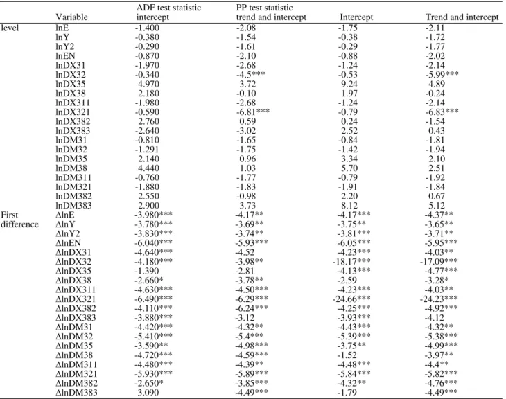
Establishing the order of integration of each variable is a concerning issue especially when working with time series data. The ARDL and FMOLS approaches are both applicable for variables that are I(0) or I(1) or fractionally integrated. The analysis begins by investigating the unit root test of variables using the augmented Dickey and Fuller (1981) ADF and Phillips and Perron (1988) PP tests. In both tests the null hypothesis of the series has a unit root is tested against the alternative of stationarity. According to the results (Table 2), all of the series appear to be integrated of order one

(I(1)), but only a few of them are stationary at levels and at the first difference. The results indicate that, none of the variable is I(2) or beyond. Hence validate the use of bounds testing for cointegration and FMOLS estimator.

After finding the integration order of the variable, F -test was done to confirm long-run or cointegration relationship between the variables. The first step in ARDL cointegration procedure is to obtain the order of lags on the first differenced variables from unrestricted Vector Autoregression (VAR) by means of Akaike Information Criterion (AIC) and Schwarz Bayesian Criterion (SBC) as the F-test is sensitive to the lag imposed on each of the first differenced variables. Therefore we follow Bahmani-Oskooee and Gelan (2006) and use AIC to select the optimum lags on each first-differenced variable. Given the number of variables and sample size in this study, optimal lag selection was done by setting the maximum lag lengths up to 1. Setting 1 as the maximum lag length helps to ensure that the degree of freedom is sufficient for econometric analysis. The F-test was done next after imposing the optimum lags on each of the first differenced variable. Thus, all reported results belong to the optimum models.

From the results of the F-tests in Table 3, it was gathered that the F statistics is greater than its critical value of 4.01 and 5.06 at the 5% and 1% level of significance respectively in seven out of eight industries that are coded 31, 35, 38, 311, 321, 382 and 383. While in industry 32, cointegration is due to the significantly negative coefficient obtained for lagged error-correction term ECMt-1 (Kremers et al., 1992; Pesaran and Pesaran, 1997; Pesaran et al., 2001) generated critical values for

F-test for sample sizes of 500 and 1000 observations. Narayan (2005) calculated critical values for sample sizes ranging from 30 to 80 observations. However, in this study, in all the cases cointegration is supported by the negative and significant coefficient obtained from lagged error-correction term. Furthermore, in some industries which cointegration is also supported by the F-statistic, there is quite large F-test relatively to the critical bound in majority of them. Given the small sample size in this study which is only 25, different critical values won’t change the results of cointegration).

Table 2. Unit root test results

ADF test statistic PP test statistic

Variable intercept trend and intercept Intercept Trend and intercept

level lnE -1.400 -2.08 -1.75 -2.11

lnY -0.380 -1.54 -0.38 -1.72

lnY2 -0.290 -1.61 -0.29 -1.77

lnEN -0.870 -2.10 -0.88 -2.02

lnDX31 -1.970 -2.68 -1.24 -2.14

lnDX32 -0.340 -4.5*** -0.53 -5.99***

lnDX35 4.970 3.72 9.24 4.89

lnDX38 2.180 -0.10 1.97 -0.24

lnDX311 -1.980 -2.68 -1.24 -2.14

lnDX321 -0.590 -6.81*** -0.79 -6.83***

lnDX382 2.760 0.59 0.24 -1.54

lnDX383 -2.640 -3.02 2.52 0.43

lnDM31 -0.810 -1.65 -0.84 -1.81

lnDM32 -1.291 -1.75 -1.42 -1.94

lnDM35 2.140 0.96 3.34 2.10

lnDM38 4.440 1.03 5.70 2.51

lnDM311 -0.760 -1.77 -0.79 -1.92

lnDM321 -1.880 -1.83 -1.91 -1.84

lnDM382 2.550 -0.98 2.20 0.67

lnDM383 2.900 3.73 8.12 5.12

First ∆_{lnE -3.980*** -4.17** -4.17*** -4.37**}

difference ∆lnY -3.780*** -3.69** -3.75** -3.65**

∆_{lnY2 -3.830*** -3.74** -3.81*** -3.71**}

∆lnEN -6.040*** -5.93*** -6.05*** -5.95***

∆_{lnDX31 -4.640*** -4.52 -4.23*** -4.03**}

∆lnDX32 -4.180*** -3.98** -18.17*** -17.09***

∆_{lnDX35 -1.390 -2.81 -4.13*** -4.77***}

∆lnDX38 -2.660* -3.78** -2.59 -3.28*

∆_{lnDX311 -4.630*** -4.50*** -4.23*** -4.03**}

∆lnDX321 -6.490*** -6.29*** -24.66*** -24.23***

∆_{lnDX382 -4.110*** -6.24*** -4.25*** -4.92***}

∆lnDX383 -3.880*** -3.12 -3.93*** -4.12

∆_{lnDM31 -4.420*** -4.32** -4.43*** -4.32**}

∆lnDM32 -5.410*** -5.4*** -5.39*** -5.38***

∆_{lnDM35 -3.590** -4.98*** -3.75** -4.99***}

∆lnDM38 -4.720*** -4.59*** -1.52 -3.97**

∆_{lnDM311 -4.480*** -4.39** -4.48*** -4.4**}

∆lnDM321 -5.930*** -5.89*** -5.84*** -5.82***

∆_{lnDM382 -2.650* -3.85*** -4.32** -4.76***}

∆lnDM383 3.090 -4.49*** -1.79 -4.49***

Note: 1. ***, ** and * are 1%, 5% and 10% of significant levels, respectively. 2. The optimal lag length was selected automatically using the Schwarz information criteria for ADF test and the bandwidth is selected using the Newey-West method for PP test. E indicates per capita carbon dioxide emissions in metric tons per capita, Y indicates per capita real GDP in constant 2000 US$, EN indicates per capita energy consumption in kg of oil equivalent, DX indicate the ratio of dirty export to China to total export and DM is the ratio of dirty imports from China to Malaysia to total imports.

Table 3. Result of ARDL cointegration test

Industry F-test ECTt-1 Result

31 Manufacture of food, beverages and tobacco 5.63*** -0.67(-2.61)** Yes

32 Textile, wearing apparel and leather industries 2.36 -0.54(-2.89)*** Yes

35 Manufacture of chemical, petroleum, coal, rubber and plastic products 5.03** -0.66(-3.54)*** Yes

38 Manufacture of fabricated metal products, machinery and equipment 5.01** -0.35(-2.60)** Yes

311 Food products 5.40*** -0.67(-2.56)** Yes

321 Textiles 4.19** -0.42(-1.93)* Yes

382 Machinery except electrical 6.10*** -0.68(-4.9)*** Yes

383 Machinery, electrical 4.41** -0.55(-2.51)** Yes

Note: 1.The critical values of F-statistics with four explanatory variables are 3.74-5.06, 2.86-4.01 and 2.45-3.52 at 1, 5 and 10% level

of significance, respectively. Pesaran et al. (2001) Table CI (iii) Unrestricted intercept and no trend. 2. The numbers in parentheses

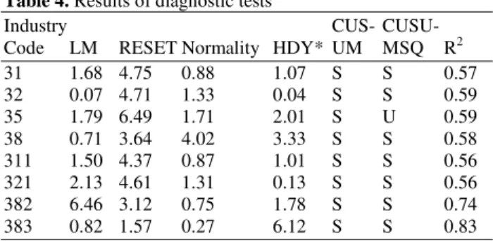
Table 4. Results of diagnostic tests

Industry CUS- CUSU-

Code LM RESET Normality HDY* UM MSQ R2

31 1.68 4.75 0.88 1.07 S S 0.57

32 0.07 4.71 1.33 0.04 S S 0.59

35 1.79 6.49 1.71 2.01 S U 0.59

38 0.71 3.64 4.02 3.33 S S 0.58

311 1.50 4.37 0.87 1.01 S S 0.56

321 2.13 4.61 1.31 0.13 S S 0.56

382 6.46 3.12 0.75 1.78 S S 0.74

383 0.82 1.57 0.27 6.12 S S 0.83

HDY = Heteroscedasticity. “S” signifies stable model and “U” signifies unstable model

Functional misspecifications do not pose any problem since RESET statistics in all cases are less than critical value of 6.63 at 10% level. Third, the estimated models also pass the diagnostic tests of normality which is distributed as x2 with two degree of freedom. Fourth, the diagnostic test statistics do not suggest the presence of any heteroskedasticity in all estimated models. This test is also distributed as x2 with one degree of freedom. Fifth, to determine stability of short-run and long-run coefficient estimates, following Pesaran et al. (2001), the CUSUM and CUSUMSQ tests were applied for the residuals of each optimal model. Stable coefficients are identified by ‘‘S’’ and unstable ones by ‘‘U’’. As can be seen, almost all estimated coefficients in all models are stable. Finally, the size of the adjusted R2 indicates a good fit in most of the models. They are more than 0.5 in all the estimated models.

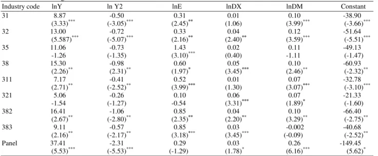
The long-run results are discussed after establishment of the cointegration relationship between variables in the selected industries. Table 5 presents the FMOLS results for Equation (1).

The positive and negative coefficients of InY and (In Y)2 respectively in all cases, suggest an inverted U-shape relationship between per capita CO2 emissions and per capita real GDP, while the coefficients of InY and (In Y)2 are statistically significant at 1% level in industries which are coded 31 and 32; at 5% level in industries which are coded 38, 311, 382 and 383 and insignificant in industries which are coded 35 and 321. The long-run elasticity of carbon dioxide emissions per capita with respect to real GDP per capita is 8.869-0.9902lnY for industry 31, 12.9957-1.4498lnY for industry 32, 15.2965-1.9528lnY for industry 38, 7.1743-0.8128lnY for industry 311, 16.4048-2.1182lnY for industry 382 and 9.1058-1.1436lnY for industry 383. Based on these results the turning points of per capita real income are calculated in logarithms. The turning points of per capita real income turned out to be 8.9567

for industry 31, 8.9638 for industry 32, 7.8331 for industry 38, 8.8266 for industry 311, 7.7447 for industry 382 and 7.9624 for industry 383 compared to the highest value of lnY in our sample which is 8.4027. Furthermore the result for the relationship between CO2 emissions and income supports the EKC hypothesis for the panel of dirty industries which trade between Malaysia and China. The calculated logarithm income level turning points of the EKC for the panel of dirty industries is 8.0915 which is lower than the highest actual value over the sample period (8.4027). This implies that the level of CO2 emissions in Malaysia increases with economic growth, then, reaches its maximum level and decreases following the income level turning point.

Table 5. FMOLS long-run estimates

Industry code lnY ln Y2 lnE lnDX lnDM Constant

31 8.87 -0.50 0.31 0.01 0.10 -38.90

(3.33)*** _(-3.05)*** _(2.45)** _{(1.06) (3.99)}*** _(-3.66)***

32 13.00 -0.72 0.33 0.04 0.12 -51.64

(5.587)*** _(-5.07)*** _(2.16)** _(2.40)** _(3.59)*** _(-5.51)***

35 11.06 -0.73 1.43 0.02 0.11 -49.13

-1.26 (-1.35) (3.10)*** _{(0.40) -1.11 (-1.47)}

38 15.30 -0.98 0.60 0.05 0.10 -60.93

(2.26)** _(2.31)** _(1.97)* _(3.45)*** _(2.46)** _(-2.32)**

311 7.17 -0.41 0.52 0.01 0.07 -32.78

(2.71)** _(-2.52)** _(3.99)*** _{(1.30) (3.07)}*** _(-3.10)***

321 5.06 -0.26 0.10 0.06 0.07 -21.33

-1.54 (-1.27) -0.54 (3.31)*** _(1.89)* _(-1.60)

382 16.41 -1.06 0.85 0.04 0.10 -66.40

(2.67)** (-2.80)** (2.35)** (2.20)** (3.29)** (-2.75)**

383 9.11 -0.57 0.85 0.03 -0.002 -40.68

(2.16)** (-2.17)** (3.18)*** (3.45)*** (-0.09) (-2.52)**

Panel 37.41 -2.31 0.29 0.03 0.26 -149.45

(5.53)*** (-5.53)*** (-1.29) (1.78)* (6.16)*** (5.62)*

Note: 1. The numbers in parentheses report t-statistics. 2. *, ** and *** represent 10%, 5% and 1% level of significance, respectively. 3. A lag length 1 of the Bartlett windows is used for the FMOLS estimator.

The consumption of renewable energy sources has been launched many times by Malaysian government through many policies and programs such as fifth fuel policy 2001, national biofuel policy 2006 and national green technology policy 2009. Malaysia is well endowed with different kind of renewable sources such as biomass, biogas, municipal waste, hydro and solar. However, Malaysia’ tropical climatic condition is more justifiable for the development of solar energy.

Remarkably, none of the import variables in Table 5

are statistically significant with a negative sign while most of them (31, 32, 38, 311, 321 and 382) are significant and positively related to CO2 emissions, which is in contrast to the PHH. This strongly rejects the PHH for CO2 emissions in Malaysia-China trade. This is consistent with the findings of Tobey (1990); Wyckoff and Roop (1994); Jaffe et al. (1995); Janickle et al. (1997); Kahn (2003) and Kearsley and Riddel (2010) who found no evidence of PHH. For the panel of dirty industries as a whole, the coefficient of dirty import is positive and highly significant at the 1% significance level. This is more emphasis on rejection of the PHH in this study.

4. CONCLUSION

This study has examined the dynamic relationship between Carbon Dioxide (CO2) emissions, economic growth and energy consumption in Malaysia for the period 1980-2004. Square of economic growth has been included to the model in order to examine the

non-linear relationship between CO2 emissions and economic growth (EKC). The evidence of Pollution Haven Hypothesis (PHH) was examined by considering the effects of dirty export from Malaysia to China and dirty import from China to Malaysia based on two and three-digit ISIC data that reflect pollution intensive manufacturing.

Energy consumption has been shown to significantly increase CO2 emissions. This can be interpreted as Malaysia is an energy dependent country that a significant amount of its economic growth is achieved through industrial growth. In 1980 about 20% of economic growth was achieved through manufacturing while in 2004 this figure increased to 30% (World Bank, world development indicator). This may increase the consumption of electricity and consequently CO2 emissions.

There is no evidence that domestic production of pollution-intensive goods in Malaysia is being replaced by imports from China. The analysis indicated that Malaysia-China bilateral trade increases CO2 emissions in Malaysia. As most of the pollution-intensive industries, specifically electrical and electronics, are leading sectors in Malaysia’s manufacturing, any changes in the volume of the trade may have negative effects on export earning, investment and employment. A more appropriate energy policy is therefore necessary. On the other hand, Levinson (2009) concludes that most of the pollution reduction in the US is due to the technology changes rather than changes in the imports or changes in the types of the domestic good production. As an example, from 1987 to 2001 the US witnessed a 25% decrease in air pollution, while maintaining the real value of manufacturing growth output at 24% (Levinson, 2009). In an emerging economy such as Malaysia, adopting a more suitable policy related to industrial production and environmental pollution is therefore very crucial particularly as a significant amount of economic growth has been fuelled by industrial growth. More efforts should also be put to use modern and cleaner technologies in the future to reduce environmental pollution.

Electricity consumption is one of the key indicators of economic growth. Electricity demand in Malaysia as an industrialized nation is expected to increases 4.7% annually by the year 2030 (Ali et al., 2012). This was mainly due to the expansion of industrial and residential sectors. Electricity generation has been always challenging. Meeting the growing electricity demand in one hand and minimizing the side effects of electricity generation on the environment on the other hand exert a heavy pressure on the countries’ government. There is a serious need in electricity generation from renewable sources which are clean, non-depleting and not emitting greenhouse gas emissions and at the same time guarantee sustainable economic growth. The drive towards the use of renewable energy sources has been launched many times by Malaysian government through many policies and programs such as Fifth Fuel Policy 2001, National Biofuel Policy 2006 and National Green Technology Policy 2009. Malaysia is well endowed with different kind of renewable sources such as biomass, biogas, municipal waste, hydro and solar. However, Malaysia’ tropical climate is suitable and justifiable for a more extensive use of solar energy. There have been some studies done on other countries that examine the effects of renewable sources specifically solar energy on EKC and on CO2 emissions mitigation, while there is no such study in the case of Malaysia. Such a project would be a worthwhile topic for future research.

5. REFERENCES

Ali, R., I. Daut and S. Taib, 2012. A review on existing and future energy sources for electrical power generation in Malaysia. Renew. Sustain. Energy

Rev., 16: 4047-4055. DOI:

10.1016/J.RSER.2012.03.003

Anderson, K. and R. Blackhurst, 1992. The Greening of World Trade Issues. 1st Edn., Harvester Wheatsheaf, New York,ISBN-10: 0745011748, pp: 276.

Ang, J., 2007. CO2 emissions, energy consumption and output in France. Energy Policy, 35: 4772-4778. DOI: 10.1016/J.ENPOL.2007.03.032

Ang, J., 2008. Economic development, pollutant emissions and energy consumption in Malaysia. J. Policy Model., 30: 271-278. DOI: 10.1016/J.JPOLMOD.2007.04.010 Antweiler, W., B.R. Copeland and M.S. Taylor, 2001. Is

free trade good for the environment? Am. Econ. Rev., 91: 877-908.

Bahmani-Oskooee, M. and A. Gelan, 2006. Testing the PPP in the non-linear STAR framework: Evidence from Africa. Econ. Bull., 6: 1-15.

Chichilnisky, C., 1994. North-South trade and the global environment. Am. Econ. Rev., 84: 851-874.

Cole, M.A. and R.J.R. Elliott, 2003. Determining the trade-environment composition effect: The role of capital, abor and environmental regulations. J. Environ. Econ. Manage., 46: 363-383. DOI: 10.1016/S0095-0696(03)00021-4

Cole, M.A., 2000. Air pollution and ‘dirty’ industries: How and why does the composition of manufacturing output change with economic development? Environ. Resource Econ., 17: 109-123. DOI: 10.1023/A:1008388221831

Cole, M.A., 2004. Trade, the pollution haven hypothesis and the environmental kuznets curve: Examining the linkages. Ecol. Econ., 48: 71-81. DOI: 10.1016/J.ECOLECON.2003.09.007

Copeland, B.R. and M.S. Taylor, 1994. Taylor MS. North-South trade and the environment. Q. J. Econ., 109: 755-787.

Copeland, B.R., 2005. Taylor and the Environment: Theory and Evidence. 1st Edn., Princeton University Press, ISBN-10: 0691124000, pp: 295.

Dickey, D.A. and W.A. Fuller, 1981. Likelihood ratio statistics for autoregressive time series with a unit root. Econometrica, 49:1057-72.

Dinda, S. and D. Coondoo, 2006. Income and emission: A panel-data based cointegration analysis. Ecol.

Econ., 57: 167-181. DOI:

Dinda, S., 2004. Environmental Kuznets curve hypothesis: A survey. Ecological Economics, 49: 431-455. DOI: 10.1016/J.ECOLECON.2004.02.011 Engle, R.F. and C.W.J. Granger, 1987. Co-integration

and error correction: Representation, estimation and testing. Econometrica, 55: 251-276.

Esty, D.C., 1994. Greening the GATT: Trade, Environment and the Future. 1st Edn., Institute for International Economics, Washington DC., ISBN-10: 0881322059, pp: 319.

Fodha, M. and O. Zaghdoud, 2010. Economic growth and pollutant emissions in Tunisia: An empirical analysis of the environmental Kuznets curve. Energy

Policy, 38: 1150-1156. DOI:

10.1016/J.ENPOL.2009.11.002

Friedl, B. and M. Getzner, 2003. Determinants of CO2 emissions in a small open economy. Ecol. Econ., 45: 133- 148. DOI: 10.1016/S0921-8009(03)00008-9 Ghosh, S., 2010. Examining carbon emissions-economic

growth nexus for India: A multivariate cointe gration approach. Energy Policy, 38: 2613-3130. DOI: 10.1016/J.ENPOL.2010.01.040

Grossman, G.M. and A.B. Krueger, 1991. Environmental Impacts of a North American Free Trade Agreement. Recent NBER Research.

Halicioglu, F., 2009. An econometric study of CO2 emissions, energy consumption, income and foreign trade in Turkey. Energy Policy, 37: 1156-1164. DOI: 10.1016/J.ENPOL.2008.11.012

He, J. and P. Richard, 2010. Environmental Kuznets curve for CO2 in Canada. Ecol. Econ., 69: 1083-1093.DOI: 10.1016/j.ecolecon.2009.11.030

Hossain, S., 2011. Panel estimation for CO2 emissions, energy consumption, economic growth, trade openness and urbanization of newly industrialized countries. Energy Policy, 39: 6991-6999. DOI: 10.1016/J.ENPOL.2011.07.042

Jaffe, A.B., S.R. Peterson, P.R. Portney and R.N. Stavins, 1995. Environmental regulation and the competitiveness of U.S. manufacturing: What does the evidence tell us? J. Econ. Literat., 33: 132-163. Jalil, A. and S.F. Mahmud, 2009. Environment kuznets

curve for CO2 emissions: A cointegration analysis. Energy Policy, 37: 5167-5172. DOI: 10.1016/J.ENPOL.2009.07.044

Janickle, M., M. Binder and H. Monch, 1997. ‘Dirty industries’: Patterns of change in industrial countries. Environ.Resour. Econ., 9: 467-491. Johansen, S. and K. Juselius, 1990. Maximum likelihood

estimation and inference on cointegration with applications to the demand for money. Oxford Bull. Econ. Stat., 52: 169-210. DOI: 10.1111/j.1468-0084.1990.mp52002003.x

Kahn, M.E., 2003. The Geography of US Pollution In tensive Trade: Evidence from 1958 to 1994. Regional Sci. Urban Econ., 33: 383-400. DOI: 10.1016/S0166-0462(02)00042-X

Kearsley, A. and M. Riddel, 2010. A further inquiry into the pollution haven hypothesis and the environmental Kuznets curve. Ecol. Econ., 65: 909-919. DOI: 10.1016/j.ecolecon.2009.11.014

Kremers, J.J., N.R. Ericson and J.J. Dolado, 1992. The power of cointegration tests. Oxford Bull. Econ. Stat., 54: 325-347. DOI: 10.1111/j.1468-0084.1992.tb00005.x

Levinson, A., 2009. Technology, international trade and pollution from US manufacturing. Am. Econ. Rev., 99: 2177-2192.

Managi, S. and P.R. Jena, 2008. Environmental productivity and Kuznets curve in India. Ecol.

Econ., 65: 432-440. DOI:

10.1016/j.ecolecon.2007.07.011

Mani, M. and D. Wheeler, 1998. In search of pollution havens? Dirty industry in the world economy, 1960 to 1995. J. Environ. Dev., 7: 215-247. DOI: 10.1177/107049659800700302

Muhammad-Sukki, F., A.B. Munir, R. Ramirez-Iniguez, S.H. Abu-Bakar and S.H.M. Yasin et al., 2012. So lar photovoltaic in Malaysia: The way forward. Renew. Sustain. Energy Rev., 16: 5232-5244. DOI: 10.1016/j.rser.2012.05.002

Narayan, P.K. and S. Narayan, 2010. Carbon dioxide and economic growth: Panel data evidence from developing countries. Energy Policy, 38: 661-666. DOI: 10.1016/j.enpol.2009.09.005

Narayan, P.K., 2005. The saving and investment nexus for China: Evidence from cointegration tests. Applied Econ., 37: 1979-1990. DOI: 10.1080/00036840500278103

Nasir, M. and F.U. Rehman, 2011. Environmental Kuznets Curve for carbon emissions in Pakistan: An empirical investigation. Energy Policy, 39: 1857-1864. DOI: 10.1016/j.enpol.2011.01.025

Ozturk, I. and A. Acaravci, 2010. CO2 emissions, energy consumption and economic growth in Turkey. Renew. Sustain. Energy Rev., 14: 3220-3225. DOI: 10.1016/j.rser.2010.07.005

Pedroni, P., 2001. Purchasing power parity tests in cointegrated panels. Rev. Econ. Stat., 83: 727-731. DOI: 10.1162/003465301753237803

Pesaran, M.H. and B. Pesaran, 1997. Working With Microfit 4.0: Interactive Econometric Analysis. 1st Edn., Oxford University Press, Oxford, ISBN-10: 0192685317, pp: 505.

Pesaran, M.H. and Y. Shin, 1999. An Autoregressive Distributed Lag Modeling Approach to Cointegration Analysis. In: Econometrics and Economic Theory in 20th Century: The Ragnar Frisch Centennial Symposium, Strom, S. (Ed.), Cambridge University Press, Cambridge.

Pesaran, M.H., Y. Shin and R.J. Smith, 2001. Bounds testing approaches to the analysis of level relationships. J. Applied Econ., 16: 289-326. DOI: 10.1002/jae.616

Phillips, P. and B. Hansen, 1990. Statistical inference in instrumental variables regression with I(1) processes. Rev. Econ. Stud., 57: 99-125.

Phillips, P. and P. Perron, 1988. Testing for a unit root in time series regression. Biometrica, 75: 335-46. Selden, T. and D. Song, 1994. Environmental quality and

development: Is there a Kuznets Curve for air pollution emissions? J. Environ. Mental Econ.

Manage., 27: 147-162. DOI:

10.1006/jeem.1994.1031

Shafik, N., 1994. Economic development and environmental quality: An econometric analysis. Oxford Econ. Papers, 46: 757-773.

Soytas, U., R. Sari and B.T. Ewing, 2007. Energy consumption, income and carbon emissions in the United States. Ecol. Econ., 62: 482-489. DOI: 10.1016/j.ecolecon.2006.07.009

Stern, D., 2004. The rise and fall of the environmental Kuznets curve. World Dev., 32: 1419-39.

Suri, V. and D. Chapman, 1998. Economic growth, trade and energy, implications for the environmental kuznets curve. Ecol. Econ., 25: 195-208. DOI: 10.1016/S0921-8009(97)00180-8

Tobey, J., 1990. The effects of domestic environmental policies on patterns of world trade: An empirical test. Kyklos, 43: 191-209. DOI: 10.1111/j.1467-6435.1990.tb00207.x

Wyckoff, A.M. and J.M. Roop, 1994. The embodiment of carbon in imports of manufactured products: Implications for international agreements on greenhouse gas emissions. Energy Policy, 22: 187-194. DOI: 10.1016/0301-4215(94)90158-9