Departamento de Informática e Matemática Aplicada Programa de Pós-Graduação em Sistemas e
Computação
An Augmented Reality Pipeline to Create
Scenes with Coherent Illumination Using
Textured Cuboids
Matheus Abrantes Gadelha
Gadelha, Matheus Abrantes.
An augmented reality pipeline to create scenes with coherent illumination using textured cuboids / Mathes Abrantes Gadelha. - Natal, 2014.
54 f.: il.
Orientador: Prof. Dr. Selan Rodrigues dos Santos.
Dissertação (Mestrado) – Universidade Federal do Rio Grande do Norte. Centro de Ciências Exatas e da Terra. Programa de Pós-Graduação em Sistemas e
Computação.
1. Computação gráfica – Dissertação. 2. Realidade aumentada realista –
Dissertação. 3. Rastreamento de características naturais – Dissertação. 4. Iluminação inversa – Dissertação. 5. Calibração fotométrica – Dissertação. I. Santos, Selan Rodrigues dos. II. Título.
An Augmented Reality Pipeline to Create Scenes with Coherent
Illumination Using Textured Cuboids
Dissertação de Mestrado apresentada ao Pro-grama de Pós-Graduação em Sistemas e Computação do Departamento de Informá-tica e MatemáInformá-tica Aplicada do Centro de Ci-ências Exatas e da Terra da Universidade Fe-deral do Rio Grande do Norte.
Orientador
Prof. Dr. Selan Rodrigues dos Santos
Universidade Federal do Rio Grande do Norte — UFRN Programa de Pós-Graduação em Sistemas e Computação — PPgSC
Natal-RN
Illumination Using Textured Cuboidsapresentada por Matheus Abrantes Gadelha e aceito pelo Programa de Pós-Graduação em Sistemas e Computação do Departamento de Infor-mática e MateInfor-mática Aplicada do Centro de Ciências Exatas e da Terra da Universidade Federal do Rio Grande do Norte, sendo aprovado por todos os membros da banca exami-nadora abaixo especificada:
Prof. Dr. Selan Rodrigues dos Santos Orientador
Departamento de Informática e Matemática Aplicada Universidade Federal do Rio Grande Norte
Prof. Dr. Bruno Motta de Carvalho
Departamento de Informática e Matemática Aplicada Universidade Federal do Rio Grande do Norte
Prof. Dr. Veronica Teichrieb
Centro de Informática Universidade Federal de Pernambuco
Agradeço fundamentalmente aos que me concederam apoio emocional e me lembra-ram, ocasionalmente, que existem tópicos importantes fora da Matemática e da Computa-ção. Aos meus amigos, meu profundo agradecimento. Especialmente a Luiz Rogério, Maria Clara, José Neto, a minha irmã, Luiza, e a principal companheira desta e de vindouras jornadas, Amanda.
Agradeço aos colegas e amigos do laboratório IMAGINA, cuja convivência foi funda-mental para a realização desse trabalho e do consequente crescimento intelectual atrelado a sua produção. Ter feito do IMAGINA meu local de trabalho foi motivo de orgulho e alegria. Muito obrigado.
Agradeço imensamente aos professores e amigos Selan dos Santos, Bruno Motta e Marcelo Siqueira. Eles me mostraram com eloquência, sagacidade e profunda dedicação, os caminhos de alegria e sofrimento que envolvem a produção científica de qualidade e relevância. O contato com eles moldou minha ótica profissional e mudou minha vida de maneira irreversível. Serei eternamente grato.
List of Figures
List of Acronyms and Abbreviations
Abstract
1 Introduction p. 12
Structure of this document . . . p. 14
2 Related work p. 15
3 DRINK: Discrete Robust INvariant Keypoints p. 19
3.1 Feature Descriptors . . . p. 20
3.2 Method . . . p. 22
3.2.1 Sampling pattern . . . p. 24
3.2.2 Choosing the test pairs . . . p. 26
3.3 Results . . . p. 26
4 Geometric Registration p. 31
4.1 Tracking Planar Objects . . . p. 31
4.2 Tracking the Cuboid Marker . . . p. 34
5 Photometric Calibration p. 38
5.1 Processing Registered Images . . . p. 39
6 Rendering p. 44
6.1 Implementation Details . . . p. 44
6.2 Rendering Results . . . p. 45
7 Conclusion p. 48
1 Photometric Augmented Reality Pipeline. . . p. 13
Chapter 2: Related work p. 15
2 Results presented in (Pessoa et al. 2012). . . p. 16
3 Results presented in (Gruber, Richter-Trummer e Schmalstieg 2012). . p. 18
Chapter 3: DRINK: Discrete Robust INvariant Keypoints p. 19
4 Plotting ofφ(x) function with different values forβ. The value empirically
chosen is highlighted (β = 0.015). . . p. 23
5 Examples of sampling patterns built based on the FREAK sampling
pattern. . . p. 25
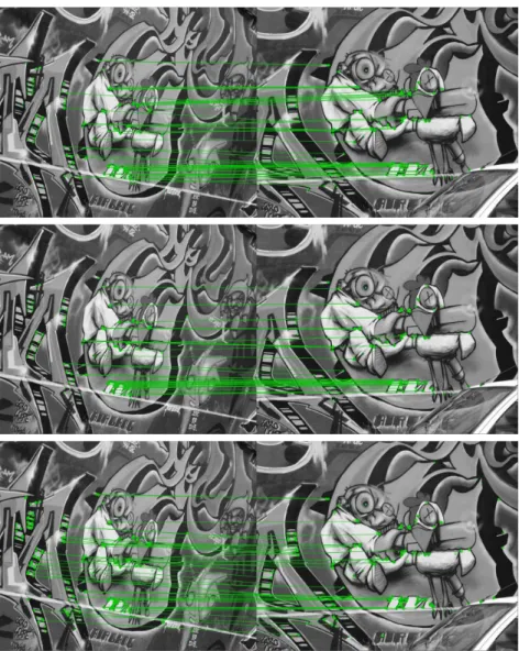
6 Matches performed using DRINK (top row), FREAK (middle row) and ORB (bottom row). We select the lowest possible threshold able to
per-form at least 40 matches. . . p. 27
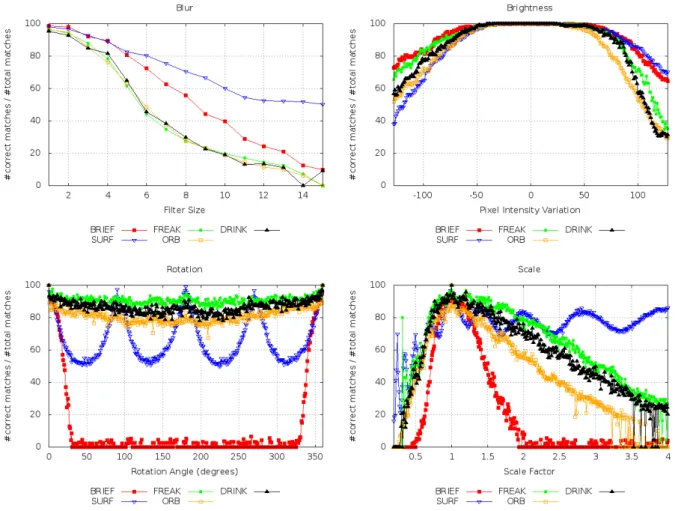
7 Comparison of feature descriptor under blur, brightness, rotation and
scale transformations. . . p. 29
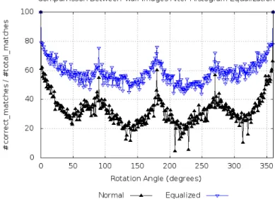
8 Comparison of precision between normal wall image and its version with histogram equalization. Images with low contrast decrease DRINK’s
ac-curacy. . . p. 30
Chapter 4: Geometric Registration p. 31
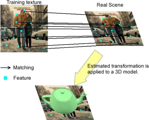
9 General steps of a NFT method. . . p. 32
10 Representation of normal sampling. . . p. 35
12 Illumination effect on planar markers. . . p. 40
13 Samples of animation frames usen in the evaluation framework . . . p. 43
14 Results obtained from the evaluation framework. . . p. 43
Chapter 6: Rendering p. 44
15 Scene generated by our method under typical lighting conditions. . . . p. 45
16 Scene generated by our method under dark lighting conditions. . . p. 46
17 Scene generated by our method when the marker is illuminated by a
flashlight. . . p. 47
AR – Augmented Reality
BRDF – Bidirectional Reflectance Distribution Functions
SIFT – Scale Invariant Feature Transform
PCA – Principal Component Analysis
BRIEF – Binary Robust Independent Elementary Features
DoG – Difference of Gaussians
SURF – Speeded Up Robust Features
FAST – Features from Accelerated Segment Test
ORB – Oriented Fast and Rotated BRIEF
BRISK – Binary Robust Invariant Scalable Keypoints
FREAK – Fast Retina Keypoints
DRINK – Discrete Robust Invariant Keypoints
OpenCV – Open Computer Vision Library
NFT – Non Fiducial Tracking
RANSAC – Random Sample Consensus
OpenGL – Open Graphihcs Library
GLSL – OpenGL Shading Language
GLM – OpenGL Math Toolkit
Iluminação Coerente Utilizando Cubóides
Texturizados como Marcadores
Autor: Matheus Abrantes Gadelha Orientador: Prof. Dr. Selan Rodrigues dos Santos
Resumo
Sombras e iluminação possuem um papel importante na síntese de cenas realistas em Computação Gráfica. A maioria dos sistemas de Realidade Aumentada rastreia marcado-res posicionados numa real, obtendo sua posição e orientação para servir como referência para o conteúdo sintético, produzindo a cena aumentada. A exibição realista de conteúdo aumentado com pistas visuais coerentes é um objetivo desejável em muitas aplicações de Realidade Aumentada. Contudo, renderizar uma cena aumentada com iluminação re-alista é um tarefa complexa. Muitas abordagens existentes dependem de uma fase de pré-processamento não automatizada para obter os parâmetros de iluminação da cena. Outras técnicas dependem de marcadores específicos que contémprobes de luz para reali-zar a estimação da iluminação do ambiente. Esse estudo se foca na criação de um método para criar aplicações de Realidade Aumentada com iluminação coerente e sombras, usando um cubóide texturizado como marcador, não requerendo fase de treinamento para prover informação acerca da iluminação do ambiente. Um marcador desse tipo pode ser facil-mente encontrado em ambientes comuns: a maioria das embalagens de produtos satisfaz essas características. Portanto, ese estudo propõe uma maneira de estimar a configuração de uma luz direcional utilizando o rastreamento de múltiplas texturas para renderizar ce-nas de Realidade Aumentada de maneira realista. Também é proposto um novo descritor de features visuais que é usado para realizar o rastreamento de múltiplas texturas. Esse descritor extende o descritor binário e é denominado descritor discreto. Ele supera o atual estado-da-arte em velocidade, enquanto mantém níveis similares de precisão.
with Coherent Illumination Using Textured Cuboids
Author: Matheus Abrantes Gadelha Advisor: Prof. Dr. Selan Rodrigues dos Santos
Abstract
Shadows and illumination play an important role when generating a realistic scene in computer graphics. Most of the Augmented Reality (AR) systems track markers placed in a real scene and retrieve their position and orientation to serve as a frame of reference for added computer generated content, thereby producing an augmented scene. Realis-tic depiction of augmented content with coherent visual cues is a desired goal in many AR applications. However, rendering an augmented scene with realistic illumination is a complex task. Many existent approaches rely on a non automated pre-processing phase to retrieve illumination parameters from the scene. Other techniques rely on specific markers that contain light probes to perform environment lighting estimation. This study aims at designing a method to create AR applications with coherent illumination and shadows, using a textured cuboid marker, that does not require a training phase to provide lighting information. Such marker may be easily found in common environments: most of product packaging satisfies such characteristics. Thus, we propose a way to estimate a directio-nal light configuration using multiple texture tracking to render AR scenes in a realistic fashion. We also propose a novel feature descriptor that is used to perform multiple tex-ture tracking. Our descriptor is an extension of the binary descriptor, named discrete descriptor, and outperforms current state-of-the-art methods in speed, while maintaining their accuracy.
1
Introduction
Augmented Reality (AR ) has been a very useful resource in areas such as Advertising, Engineering, Education, Medicine, Architecture, etc. AR allows applications to add regis-tered virtual content to the real world, thus creating an augmented environment where synthetic and real information coexist (Azuma 1997). Therefore, it is necessary to gather information from the real world to mix virtual and real content properly. Since real world information usually comes from a set of images captured from a camera, computer vision techniques play an important role in generating a mixed scene. Furthermore, real time interaction is a key feature in AR applications and processing camera images to retrieve information for a proper registration is not a simple task. To simplify this task, AR ap-plications usually insert easy-to-track markers in the real scene they wish to augment. Tracking these markers is important to estimate all characteristics of the virtual content affected by the real environment.
Realistic lighting, shading and shadow casting are important aspects that improve the degree of realism in a computer generated photorealistic scene. However, most of the current AR applications limit themselves to extract position and orientation information to aid the registration process and render their content based only on a local lighting model, usually producing incoherent illumination results. To render a virtual object with an illumination similar to a real environment, it is necessary to identify the environment’s lighting configuration. This task is called inverse rendering, or photometric calibration. Another issue arises from the fact that AR applications require real time interaction. Thus, such systems need to perform photometric calibration very fast. Besides rendering scenes with an illumination similar to the real world, a robust AR pipeline needs to be able to react to illumination changes. In other words, for each rendered frame it is necessary to process a camera frame to properly compute an approximate real illumination configuration.
other methods require a non-automated training phase to perform photometric calibration (Pilet et al. 2006) (Aittala 2010) (Jachnik, Newcombe e Davison 2012). From now on, we will refer to an AR pipeline able to perform photometric calibration as a Photometric AR Pipeline.
At this point, we are able to summarize the following desired characteristics of a Photometric AR Pipeline: a) to react to environment illumination changes in real time; b) to perform on-the-fly photometric calibration; and c) to seamlessly integrate with current AR applications, without requiring extra hardware. The purpose of this study is to create an Photometric AR Pipeline that fullfils all these conditions. To accomplish this task, we rely on a volumetric marker: a textured cuboid. Most of manufactured product packaging have these characteristics.
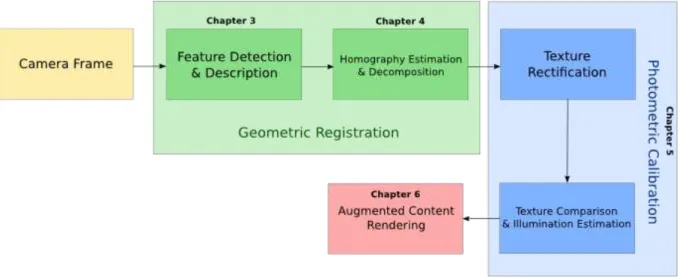
A traditional AR pipeline consists of several stages, even if it is only performing geometric registration. Our work adds extra stages in order to perform photometric ca-libration. Besides estimating environment illumination, it is necessary to properly adapt the augmented content rendering to represent such calculation. A scheme representing our proposed Photometric Augmented Reality Pipeline is outlined in Figure . Each stage of the reffered pipeline will be detailed in other chapters of this document.
Figura 1: Visual scheme representing the proposed Photometric Augmented Reality Pi-peline.
AR pipeline to perform photometric calibration using a textured cuboid as a marker. This stages enables augmented content rendering with an improved degree of realism.
Structure of this document
2
Related work
The work presented here proposes a complete AR pipeline to generate scenes with re-alistic illumination. There are several ways to accomplish this task. The works of Debevec (1998) and Debevec and Malik (1997) presented pioneer approaches for the problem of retrieving lighting parameters from a real scene. The method proposed in (Debevec 1998) uses a mirrored sphere and high dynamic range images in order to construct a coherent light-based model. This work creates scenes with synthetic elements, but does not support real-time interaction. An application of this method in the AR context can be found in (Agusanto et al. 2003).
Figura 2: Results presented in (Pessoa et al. 2010).
Pilet and collaborators (2006) present a geometric and photometric camera calibration technique that generates AR scenes with coherent illumination. However, this method presents two drawbacks: it relies on the use of multiple cameras, and requires a training phase where a marker needs to be rotated in front of the camera set. The photometric calibration is performed by sampling marker color intensities as the marker’s orientation changes. The marker orientation may be associated with a single normal vector (for the case of planar markers). To create diffuse illumination maps, all normals of the visible hemisphere should be sampled. However, this is not necessary because some non-sampled directions can be inferred by interpolating known ones.
located in the scene. Besides using the mirrored sphere as a texture applied on the virtual objects, this technique creates virtual objects with a mirrored surface. Notwithstanding, this configuration may disrupt user interaction, since it is necessary to include a mirrored sphere in the real world. Nowrouzezahrai and collaborators (2011) also use a mirrored sphere when creating realistic renderings with mixed-frequency shadows in AR.
Aittala (2010) presented a work similar to (Pilet et al. 2006), in which they managed to avoid the need of multiple cameras. Photometric calibration could be performed by a white lambertian sphere or by rotating a marker in front of the camera. Nevertheless, such training phase or custom object may be prohibitive to some kinds of AR application, like advertisement, and a lambertian sphere may not always be available. This approach also relies on constructing light maps from different evaluated normals. But, instead of computing illumination as a set of directional lights, Aittala (2010) uses a set of point lights. These lights are composed to approximate real scene illumination.
Jachnik and collaborators (2012) also describe a way to perform photometric calibra-tion from a single RGB camera. However, while other approaches use a simple diffuse illumination model, this work estimates environment light configuration from specular reflections on tracked surfaces. This approach requires a training phase where different camera views of the static marker need to be sampled.
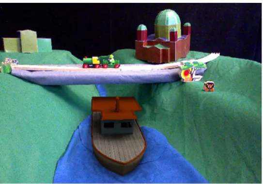
Figura 3: Results presented in (Gruber, Richter-Trummer e Schmalstieg 2012). The boat is a virtual object.
3
DRINK: Discrete Robust INvariant
Keypoints
Describing image features is the first step of an Augmented Reality pipe-line that does not relies on fiducial markers. This task is also an important part of many Computer Vision related tasks, like object recognition and matching (Bo et al. 2011), motion tracking (Gomes, Carvalho e Gonçalves 2013) and 3D scene re-construction (Tola, Lepetit e Fua 2010). This chapter presents a novel feature descriptor (Gadelha e Carvalho 2014) which is faster than current state-of-the-art methods and has similar or better precision under several image transformations. Another advantage of the proposed method is that is possible to parameterize the tradeoff between precision and speed, by increasing the number of bits used per pixel intesity comparison. By using this novel descriptor, we were able to speed up early stages of our AR pipeline and to increase geometric registration precision. A good feature descriptor is capable of providing inva-riance to geometric and lightining transformations while consuming as few memory as possible. During the past decades, many efforts have been made towards achieving this goal.
However, since binary descriptors only store a single bit per pixel comparison, they only record the information if a pixel intensity is larger (smaller) than the intensity of another pixel. Thus, a useful portion of information, about how large that difference is, is lost due to this quantization.
The power behind the binary descriptors comes from the hundreds of intensity compa-risons that are performed, providing them robustness under several image transformations. However, those descriptors can be significantly improved by providing them with more information regarding to the difference between the pixel intensities. Our study proposes a generalization of the binary descriptor, by creating a discrete data structure that takes into account the difference between pixel intensities while preserving the characteristics that enable a fast matching.
This chapter is organized as follows. Section 3.1 describes related works, while Section 3.2 describes the proposed method and its implementation. Finally, Section 3.3 shows the results obtained by the proposed method in comparison to other descriptors, as well as the results of an experiment dealing with a real matching situation.
3.1
Feature Descriptors
Another descriptor that also relies on local gradient histograms is SURF (Spe-eded Up Robust Features) (Bay et al. 2008). The SURF presents a close matching to the performance of SIFT, while significantly decreasing its computational time (Bauer, SÃijnderhauf e Protzel 2007). Its feature detection technique uses the determi-nant of the Hessian matrix to identify image blobs. The SURF descriptor is then com-puted by summing Haar wavelet responses at the region of interest. Similarly to what is done in SIFT, SURF relies on floating-point calculations. This fact has a great impact on the computational time spent by these methods. Usually, the measure of distance between two floating-point based descriptors is computed using the Euclidean distance, which in-creases the time spent computing the descriptors. This is the main point attacked by the descriptors based on binary strings to speedup their computation.
A binary descriptor consists of a binary string whose values are filled based on intensity comparisons of pixels located in the region of interest. The first binary descriptor proposed was BRIEF (Binary Robust Independent Elementary Features) (Calonder et al. 2012). An important advantage of this type of descriptors is that the measure of distance between two binary descriptors can be performed by the calculation of the Hamming distance. Computationally, this corresponds to a bitwise XOR followed by a bit count. Furthermore, the descriptor computation itself is faster than the floating-point based descriptors, since a binary descriptor only consists on a series of results from a set of fixed comparisons (the fixed-point values correspond to pixel intensities, usually a 8-bit data type). To provide robustness to noise, the region of interest is smoothed before performing such comparisons.
However, while BRIEF is really fast, it is not robust to scale and rotation variati-ons. Following the appearance of BRIEF, several binary descriptors were proposed, such as ORB (Oriented FAST and Rotated BRIEF) (Rublee et al. 2011), that presents an alternative to provide tolerance to those changes. The ORB’s keypoint detector uses the FAST (Rosten e Drummond 2006) corner detector with pyramidal schemes to pro-vide scale information to features (Klein e Murray 2008). It also uses Harris corner filter (Harris e Stephens 1988) to reject edges and provide reasonable scores, and the intensity centroid calculation to compute keypoint orientations, as proposed by Rosin (Rosin 1999).
is similar to the one adopted by DAISY (Tola, Lepetit e Fua 2010).
Similarly to the work proposed here and to BRIEF, FREAK (Fast Retina Keypoint) (Vandergheynst, Ortiz e Alahi 2012) presents a descriptor decoupled from a keypoint de-tector. The approach adopted by FREAK is closely related to BRISK, differing only on the geometric pattern chosen to perform the binary tests and on how those test pairs are selected. FREAK uses a geometric pattern that mimics how the human retina works and its test pairs are selected through training, similar to the method used by ORB.
This work extends the binary descriptors idea while preserving the characteristics that make them faster than the floating-point based descriptors. We will rely on the previous advances made on the binary descriptors, such as the retina-like geometric pattern from FREAK and the ORB feature orientation.
3.2
Method
Binary descriptors are formed by putting together strings of bits whose values are determined by binary tests comparing two pixel intensities. Let I(p) be a function that returns the smoothed intensity of a region (to be defined later) centered at a pixelp and
Pa be the pair of pixels Pa1 and Pa2. Then, the binary test T(Pa) of a pixel pair Pa is
defined as:
T(Pa) =
1 if (I(Pa1)−I(Pa2))≥0 0 if otherwise.
(3.1)
Then, a complete binary descriptor of size N can be formed by concatenating N
binary test results. Finally, a binary descriptor B is defined as:
B =
N−1
X
a=0
2aT(P
a). (3.2)
However, Equation 3.1 shows that the difference between two intensities (I(Pa1) and
I(P2
a)) is mapped onto a single bit. A trivial way of considering more information from
BRIEF would occupy 512 bytes, instead of 32. Thus, we need a different way to quantize this difference.
Our approach consists in generalizing the binary descriptors to bek-ary descriptors by quantizing the intensity difference intokvalues. Therefore, we need a functionφ(x) to map anx value (in the range [−L, L], whereLis the maximum intensity level allowed, usually 255) into the range [0, k). The simplest way to do that is by defining φ(x) as a linear function. However, we noticed that such distribution reduces the number of occurrences of extreme values ofφ(x). In other words, definingφ(x) as a linear function implies in an increased number of results in the middle of the interval [0, k). This characteristic reduces the discriminating power of our descriptors. That is why we defined φ(x) as the sigmoid function:
φ(x) = βkx
2q1 + (βx)2 +
k
2, (3.3)
where β is a “stretching” coefficient, used to reduce or increase the amount of extreme values obtained. We chose empirically the value ofβ to be 0.015. To illustrate the behavior of this function as we change the β, in Figure 4 we plot the curves for this function for
k= 5 and different values of β.
The φ function is a way to perform the quantization of the difference between two intensities intok values. Our task is to create a discrete descriptor that takes into account those differences, preserving the possibility to measure the distance between two descrip-tors by Hamming distance. The idea is to represent each intensity difference as a binary string of size k−1. For example, if k = 5 and the I(P1
a)−I(Pa2) = −255 the resulting
binary string is 0000. Though, ifI(P1
a)−I(Pa2) = 255, the binary string that represents
this value is 1111. As a middle term, if we have I(Pa1)−I(Pa2) = 0 our resulting binary string corresponds to 0011. By doing this, even though we do not use all possible binary values that can be represented byk bits, we can still use the Hamming distance to com-pute the distance between two descriptors. Finally, we can define aD discrete descriptor as:
D=
N−1
X
a=0
2a(k−1)
⌊φ(I(P1
a)−I(P
2
a))⌋−1
X
i=0
2i
. (3.4)
It is important to notice that if we choosek = 2, there are only two possible values for ⌊φ(I(Pa1)−I(Pa2))⌋: 0 or 1. As a consequence, the second sum in Equation 3.4 will generate these same values. Therefore, whenk = 2,Dcorresponds to the binary descriptor defined at Equation 3.2.
3.2.1
Sampling pattern
Our method uses a circular sampling pattern similar to the ones used by FREAK, BRISK and DAISY. However, in later two methods, the points are equally spaced on concentric circles, as opposed to the sampling pattern adopted by FREAK, which aims to mimic the human retina by having a higher density of points near the center (Vandergheynst, Ortiz e Alahi 2012).
Binary descriptors perform smoothing of the sample points to make the intensity tests less sensitive to noise. The ORB and BRIEF use the same kernel for all sample points, as opposed to BRISK and FREAK, that use variable kernels, with the changes in kernel size being much bigger in FREAK than in BRISK. FREAK also allows that the receptive fields overlap. According to (Vandergheynst, Ortiz e Alahi 2012), those characteristics increase the descriptor performance.
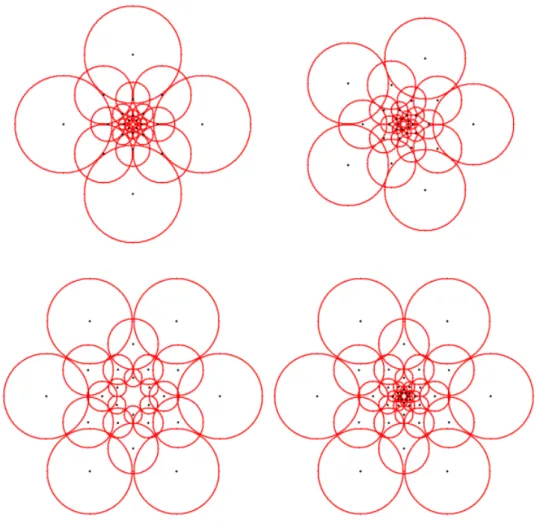
per-Figura 5: Examples of sampling patterns built based on the FREAK sampling pattern. The red cirles represent the size of the Gaussian kernel used in the smoothing process. The black dots show the center of those regions. The upper left pattern consists of 5 levels, each one with 4 receptive fields. The upper right pattern consists of 5 levels, each one with 5 receptive fields. The bottom left pattern consists of 4 levels, each one with 6 receptive fields. The bottom right pattern consists of 7 levels, each one with 6 receptive fields.
3.2.2
Choosing the test pairs
In order to choose the best test pairs among all the sampling points, we used an approach similar to the one used in ORB (Rublee et al. 2011). We do that by setting up a training set of approximately 300k keypoints, drawn from images in the PASCAL 2006 set (Everingham 2006). Then, we compute a descriptor composed of all possible test pairs for each keypoint. From this information, we are able to create a matrix whose columns are associated to the test pairs and the lines are associated to the keypoints. Each element of this matrix contains a result from 0 tok−1, computer using the floor of value computed by Equation 3.3. Then, we execute the following algorithm to choose the best test pairs.
1. Sort the matrix columns according to their entropy (Gonzalez e Woods 2006), from the highest value to the lowest one.
2. Add the pair corresponding to the first column (highest entropy) to the set P of best pairs.
3. For each column in the matrix (traversing it according to order defined in Step 1), compute its correlation to the column associated with each element of the P set. If this correlation is lower than a thresholdtfor all elements inP, insert the associated pair in P.
• If there are enough pairs in P stop the algorithm.
4. If every column has been tested and there are not enough elements in P raise the value of t and repeat this algorithm again.
3.3
Results
The tests were executed using a Desktop PC with an Intel i7 2.5 GHz processor and 8 GB of RAM. All methods were tested using the respective versions available at OpenCV 2.4.7. The DRINK implementation was built under the same OpenCV framework. Thus, there are no gains of speed due to the software architecture.
Our experiments were conducted on a framework similar to the one presented at (Barandiaran et al. 2013) and the approach
Figura 6: Matches performed using DRINK (top row), FREAK (middle row) and ORB (bottom row). We select the lowest possible threshold able to perform at least 40 matches.
feature-descriptor-comparison-report/. The strategy consists of
ap-plying rotation, scale, brightness and blurring transformations to an image from the Mikolajczyk and Schmid data set (Mikolajczyk e Schmid 2005). By doing this, we are able to verify the robustness of our method to each transformation separately. In all results presented here, we used a sampling pattern that mimics FREAK, but with 7 levels, each one with 6 receptive fields. This corresponds to the pattern on the bottom right of Figure 5. We are also using 64 test pairs, quantizing the difference in 5 values (k = 5).
same descriptor length, or apply a threshold value two times greater for FREAK (since it uses two times more bits), no matches are obtained. This means that the distances of the real matches computed by ORB and FREAK are larger than the ones computed by DRINK. Our experiments also show that the results produced by DRINK have similar or better precision level than other widely used binary descriptors and it is more than 3 times faster than ORB and about 20% faster than FREAK, while spending half of its bits to store a descriptor.
Tabela 1: Average times (in microseconds) per keypoint used in keypoint detection, des-criptor computation and matching (Total) and in the desdes-criptor computation alone (Des-cription).
Avg. Time SURF BRIEF ORB FREAK DRINK
Total 350.32 34.273 45.290 52.793 41.807 Description 204.73 3.7249 15.78 6.176 4.8140
Figure 7 show the comparison of FREAK, SURF, BRIEF, ORB and DRINK per-formance under blur, brightness, rotation and scale transformations, respectively. The keypoint detector used in was the same used by ORB, due to its high speed and good repeatability rate (Miksik e Mikolajczyk 2012). However, since SURF presented poor re-cognition rates under those circumstances, we choose to display the results obtained from its original framework, using keypoints detected by SURF algorithm.
Under all transformations tests, DRINK presented similar performance to FREAK and ORB, being slightly worse than FREAK and better than ORB in all circumstances, except in the blurring transformations, where all 3 descriptors presented a similar beha-vior. However, as we can see in Table 1, DRINK is reasonably faster than FREAK and ORB. This is explained by the fact that DRINK is performing only 64 tests when FREAK uses 512 and ORB, 256. It is important to note that DRINK’s performance could be even better if more test pairs were used. We experimentally determined 64 as the number of pairs because it produces a good trade-off between precision and speed.
We can also see in Table 1 that the description time of ORB is larger than the one for FREAK, but the total computation time of ORB is smaller than the one of FREAK. This happens because the ORB descriptor has 256 bits while the FREAK descriptor has 512 bits.
Figura 7: Comparison of feature descriptor under blur, brightness, rotation and scale transformations.
4
Geometric Registration
To generate an augmented scene, a typical AR application normally works in three steps. First, it receives as input a video streaming of the real world and applies Computer Vision algorithms to recognize all the pre-defined markers that are visible in a given frame. Secondly, the application must calculate the camera pose—i.e. position and orientation— based on the relative location of the markers within the image frame. The end result of this step is a list of coordinate system of reference associated to each deteced marker. Thirdly, the AR application should register the augmented content (i.e. the computer generated content) to each coordinate system of reference found in the previous step. In other words, given an image containing a marker, we need to perform a reverse process to retrieve the position and orientation of the real camera so we can determine the geometric transformation (homography) necessary to align the virtual and real cameras.
The AR method proposed in this document tracks a textured cuboid marker, instead of the traditional textured planar marker. We have chosen a volumetric marker for two reasons: i) a textured box may be considered an universal item ordinarily found in our home or workplace, as it is the case of most product packaging, and; ii) a volumetric marker would help us to execute a photometric calibration without a training phase—in particular, a cube may provide up to three normal vectors, depending on the angle the cube is facing the camera.
The next section presents a general description of the process involved in tracking a planar marker. The last section presents an efficient approach to track multiple textures after determining their geometric interrelationship.
4.1
Tracking Planar Objects
which estimate camera pose based on the points extracted from planes in the environ-ment (Simon e Berger 2002, Lourakis e Argyros 2004). To accomplish efficient pose esti-mation it is important to identify good “interesting” or “key points” to track. The set of interesting points on an image is known as the feature description. For a tracking te-chnique to be considered robust it is necessary that the image’s feature description be detectable even after the image has undergone changes in orientation, scale, and bright-ness, for instance. Therefore, the key points often correspond to high-contrast regions of the image.
Point descriptors may be loosely defined as a generic data structure that encodes the location and characteristics of interest points within a target image. The matching of the target and reference images are based on some method-dependent metric for these pre-computed point descriptors. This matching task is commonly referred to as Non-Fiducial Tracking (NFT) in the AR literature (Calonder et al. 2012, Wagner et al. 2008, Simon e Berger 2002, Bastos e Dias 2005). Figure 9 shows an overview of the general steps commonly found in Non-Fiducial Tracking (NFT) methods.
Figura 9: General steps of a NFT method.
orientation with respect to the camera frame that generated thetarget image. Evey time we mention a marker in this document we are actually referring to thereference image or textureassociated with it. We may summarize the tracking process through the following steps (Wagner et al. 2008).
1. Pre-process the marker we wish to track, computing and storing itsfeature descrip-tors (f dm)
2. Obtain an input target image where the marker may be found; in the AR context, this often means to capture images from a digital camera.
3. Process the target image, computing and storing its feature descriptors (f dti).
4. Try to match the marker’s feature descriptors (f dm) and the target image (f dti).
5. Identify the geometric transformation that leads the “key points” from the marker to the matched “key points” in the target image.
6. Determine the position and orientation for the augmented content based on the geometric transformation found in the previous step.
These steps must be repeated for each rendering frame of the application’s graphics pipeline. Thus, they have to be executed very efficiently if we wish to keep real time frame rates.
In our proposed aproach, we will use the ORB feature extractor (Rublee et al. 2011) along with the DRINK descriptor, explained in the previous chapter, in order to estimate the geometric transformation matrix. The DRINK descriptor was cho-sen because it is faster to calculate and requires less memory than other similar methods, such as FREAK (Vandergheynst, Ortiz e Alahi 2012), SURF (He et al. 2009), or Ferns (Ozuysal et al. 2010). These characteristics found in DRINK descriptors were decisive for our approach since that in the worst case our cuboid marker would have six different textures on its faces. In this case we would need to quickly calculate and keep six different descriptors sets, one for each face of the cuboid marker.
Once we have found a proper match between a marker and a target image, we need to find a perspective transformation that leads the “key points” from the marker to the target image. Such affine geometric transformation is called homography. A homography is an invertible transformation from a projective space to itself. Therefore, assuming a pinhole camera model, any two images of the same planar surface are related by an homography. Considering that a homography is a linear transformation we present the following equation:
ps =Hpr (4.1)
wherepr is a reference image point expressed in homogeneous coordinates,ps the
corres-ponding point in the scene image andHthe homography matrix. From 4.1, we define the problem of finding an homography matrix from a set of P correspondences as:
argmin
H
X
(ps,pr)∈P
kps−Hprk2. (4.2)
However, there are usually incorrect matches between the scene points and the refe-rence image points (outliers). Thus, we need to use a method capable of reducing outliers, called RANSAC (Fischler e Bolles 1981). It produces a model which is only computed from the inliers, provided that the probability of choosing only inliers in the selection of data is sufficiently high. Using the camera intrinsic parameters we are able to extract a rotation matrix R and a translation vector ~t. (Malis e Vargas 2007) present a set of methods to perform this task. In our particular case, we use a method that solves an opti-mization problem that minimizes reprojection error. Such function is available in OpenCV assolvePnP (Bradski e Kaehler 2008).
4.2
Tracking the Cuboid Marker
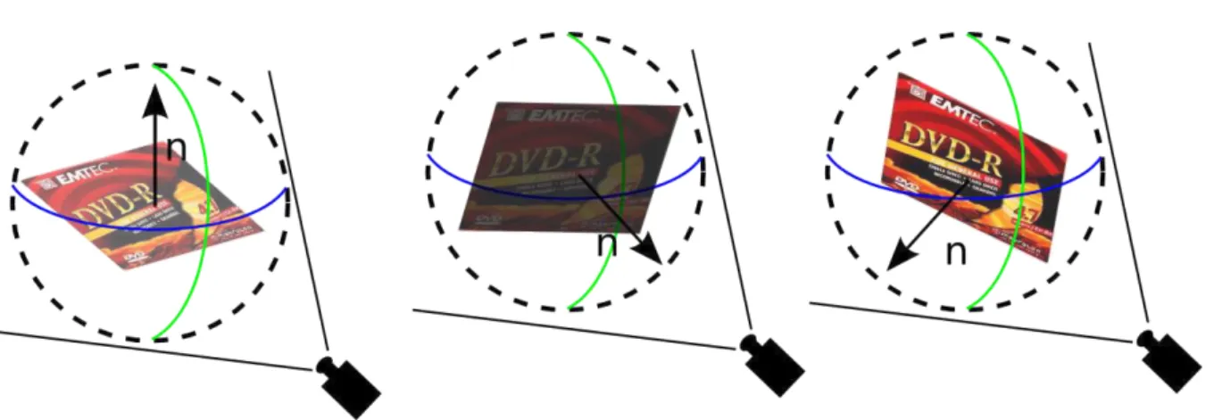
Figura 10: Representation of normal sampling. The intensity of one directional light is associated with the marker color, while its direction is associated with the marker normal vector.
Tracking a cuboid marker is a task that can be simplified by tracking its individual faces. A brute-force approach will track each one of the visible faces independently, gene-rating different homography matrices. This naive approach, although technically correct, is not very efficient. Considering that we know in advance the geometry of our marker, we only need to track one face of the object. The other faces can be found by applying the transformation relative to the tracked face.
Considering a pinhole camera model, a scene view is formed by projecting 3D points into the image plane using a perspective transformation. A projected points on the scene view is described by the following equation:
s=K[R|t]S (4.3)
where S is the point in the real world, K the camera intrinsic matrix, R the rotation matrix and t is the translation column vector. Expanding Equation 4.3, we have:
u v 1 =
fx 0 cx
0 fy cy
0 0 1
r11 r12 r13 t1 r21 r22 r23 t2 r31 r32 r33 t3
X Y Z 1 (4.4)
wherefxand fy are focal lengths expressed in pixel-related units and (cx, cy) is a principal
point (that is usually at the image center). Those are calledcamera intrinsic parameters.
The camera intrinsic parameters never change during the tracking process and are related only to the device used to collect the input images. When a single face of the cube is correctly tracked, we can estimate the extrinsic parameters for that face by decomposing the homography matrix. We need this information to register virtual content properly. However, as mentioned before, it is also necessary to register the cube’s faces from the real scene on the reference images. In other words, we need to find a homography matrix that will map the desired cube face (on the real scene) to the associated reference image. This is a trivial task, considering we have all the extrinsic parameters. Plugging in the points (in world coordinates) corresponding to the vertices of the face in Equation 4.4, we find 4 points expressed in image coordinates that can be associated to the corners of the reference image. After the determination of these 4 reference points, the homography can be found by solving Equation 4.2.
Another optimization can be done on the face registration step. At least three faces of a cube are not visible when capturing its image from a camera. The registered faces of the cube are the input information for the photometric calibration. Such process is done by comparing the pixel intensities of the reference images with the registered ones. Therefore, there is no reason to perform image registration on invisible faces. We need an algorithm to check if a face of the cube is being occluded by another face. Notice, however, that any occlusion generated by other objects present in the scene may compromise the photometric calibration process since our method currently cannot handle occlusion caused by other objects.
To test a face for self-occlusion, we will use the following procedure. From a set F of faces, we want to generate two disjoint sets corresponding to the invisible faces (N) and to the visible faces (V). Both sets (N andV) are empty in the beginning of our procedure. The first element of each set is defined by using the technique described at Section 4.1: Search for a face inF; when a face fi is found, we insert fi in V and its opposite face is
inserted inN. The previous step is repeated until a face is found. When we have at least one element atV, we deduce the pertinence of the other elements in F by the following criteria. Let f0 be the first visible face found. Let fk be the face that we want to check
its visibility. Let Pf0 and Pfk be the set points corresponding to the vertices of f0 and
fk, respectively, in image space coordinates, found by Equation 4.4. To determine iffk is
visible, we check if the polygon delimited by Pfk intersects the polygon delimited by the
Figura 11: Representation of the process of defining visible faces.fkrepresents an invisible
face. f0 represents a visible face. The yellow area shows the intersection between both
faces.
5
Photometric Calibration
The analysis of the texture color intensities associated with a marker under various distinct orientations is an important step in the process of photometric calibration. One way to describe the diffuse illumination of a scene is to associate each normal on the camera visible hemisphere with a directional light. Comparing texture color intensities in different orientations is an efficient way to estimate the configuration of those lights. Previous works (Pilet et al. 2006, Aittala 2010) have managed to sample those intensities by relying on training phases where the marker is manually rotated and those samples are extracted. We overcome this drawback by inserting a marker that allows multiple normal sampling in a single frame: a cuboid with faces composed by textured planar markers.
After the Geometric Registration step, described in Chapter 3, we are able to de-termine a set R of visible faces on our cubic marker (“registered images”) and their corresponding normal vectors, given atarget image. The goal of the next step, called Pho-tometric Calibration, is to compare R with the corresponding set T of original textures from the cuboid marker. Notice that all the images of the setT are stored once, before the whole tracking process begins, and they represent the texture albedo of each one of the cube’s faces. By texture albedo we mean the natural color of the image texture, without the influence of local illumination. On the other hand, R is a subset of images from T that have been affected by the lighting conditions found on the real world scene we want to augment.
Our proposed method determines the lighting parameters of the scene based on the pixel intensity difference between the corresponding images of theRandT sets, weighted by the normals associated with each element of R, which, in turn, have been calculated during the previous Geometric Registration step.
5.1
Processing Registered Images
When the cube’s faces are tracked, an homography matrix that leads from thetexture to the target image is computed. Applying the inverse of this transformation on the real scene will generate a registered version of the scene. This new image will correspond to the marker’stexture, but its color will be affected by the environment illuminations. Thus, by comparing both images we are able to identify the influence of the illumination on the tracked marker. The objective of such comparison is to generate a data structure that describes how the markers are illuminated. This data structure will be the input data to our optimization problem.
The first step to perform this comparison is to scale down both images. It has two pur-poses: improve robustness to small localization errors resulting from the image acquisition process and speed up further processing. We use a scale factor of 0.1 in our implementa-rion. However, considering this step is done regarding performance issues, depending on the size of the original images, this value may change. A future work is to determine an optimum value of the scale factor according to the characteristics of each image. For now on, we will refer to the pixels of these images as patches.
Now, it is necessary to understand how the illumination interacts to the marker to generate the registered image. Considering the texture as the surface albedo and the registered image an illuminated version of it, we need to retrieve how the illumination is distributed on that surface. Using a diffuse illumination model, the color of the pixel π
on the registered imager is given by the equation:
rπ =σπaπ
where σ is a vector representing the irradiance color and intensity, and a is the image albedo. Here, our objective is to findσ, thus we may write the previous equation as:
σπ =
rπ
aπ
(5.1)
Figura 12: Illumination effect on planar markers. The first row presents target images. The second row shows registered images after down scale. The third row images were generated by the values ofσπ from Equation 5.1.
5.2
Illumination Estimation
In this study we are assuming a simple illumination model composed only by a single directional light and an environment component. This model is a simple approximation to the real world illumination. However, approximating this configuration we are able to achieve a good rendering quality by creating BRDF materials and shadow effects. To describe the illumination of our augmented scene, we need to estimate three values belonging to R3: the color of the ambient component (Ia), the direction of a directional
light (d~) and its color (Id).
to the cosine of the angle between the illuminating source and the normal. Therefore, we assume that a face of the cuboid marker gets more illuminated as its normal direction gets similar to the direction of the light. Thus, our method estimates the directional light by summing all the face’s normals weighted by their average irradianceσ¯. Considering that a registered image t was divided in N patches, we may calculate σ¯t using the following
equation:
¯
σt= π∈t
P rπ
aπ
N (5.2)
notice that since rπ and aπ are color values belonging to R3, rπ
aπ is a component-wise
division.
Using the avarage irradiance obtained from Equation 5.2, we may now estimate the directional light d~:
~ d=
t∈R
X
kσ¯tk~nt (5.3)
where~nt is the normal of the facet and R the set of registered visible faces. Notice that
¯
σt is a color value belonging toR3. However, we need a single real value in Equation 5.3.
Thus, we calculate the weight of the normal ~nt as the L2 norm of σ¯t. We also use ¯σt
values to assign the directional light color and the ambient color. This process consists of ordering σ¯t values according to their L2 norm kσ¯tk. The lowest value corresponds to the
ambient color Ia, while the highest corresponds to the directional light color Id.
The method described above is able to successfully estimate the directional light configurarion and the color of an ambient component. Nevertheless, such method relies on pixel values of the registered images originated from a digital camera. Thus, those images present wrong pixel values due to the noise from the acquisition device and registration error. Besides, those wrong color values may also occur when the markers are occluded by hands during manipulation. Therefore, we need to select which patches to use when computing values of σ¯t by Equation 5.2. This procedure happens as follows. Firstly, we
apply a squared gaussian filter of size 5 in images r and a. Secondly, we define a new imager′ by using the following equation:
r′(~x) =|r(~x)−a(~x)|
where r′(~x) is the color of the image r′ in the coordinate ~x. Notice that |r(~x)−a(~x)| is
a component-wise absolute value of the subtraction of the color r(~x) by the color a(~x). Thirdly, we define a new single-channel image m:
Finally, we select the patches in the coordinate ~x, such that m(~x) < k, where k is an arbitrary threshold value. In our implementation,k = 30. We are able to summarize the computation of the directional light in Equation 5.4:
~ d= t∈R X
π∈t|mπ<k
P rπ
aπ Nk
~nt (5.4)
whereNk is the number of patches π∈t whose values are smaller than k.
5.3
Evaluation Framework
The method presented in this study to perform photometric calibration uses a rough illumination model that only approximates real circunstances, but it is good enough to mimic the real world and provide a coherent illumination to the augmented content. As mentioned in previous section, our model relies on a single directional light and an ambient component. However, we would not be able to measure how precise our technique is, because there is no ambient component nor directional light in real conditions. Thus, we have generated a synthetic animation containing a textured cuboid illuminated by a single directional light and environmental component.
This animation was created using the Unity3D engine, version 4.2. The faces of the cuboid were extracted from photographs of a real world book, in order to simulate a plausible marker. We also choose a book due to the characteristics of its side faces: they are basically white (pages of the book) and therefore cannot be tracked by our pattern recognition technique. This obligates our method to track only the cover of the book, simulating a worst-case situation, when only one of the cuboid faces can be tracked (the cover of the book). Such configuration designedly increases the registration error, testing our noise and geometric calibration error handling solution. We also rotated the virtual book around the Y and X axis in order to make the side faces visible. In real circunstances, when a face is not visible, we use its last computed weight when computing the light direction. If a face was never visible, we simply consider the weight of its normal as zero.
Figura 13: Samples of animation frames usen in the evaluation framework. From left to right: frames 1, 56, 140 and 270.
directional light, while the side faces only present ambient component. Figure 14 presents the results of the estimation as coordinates of a unit vector representing the direction of the directional light. As we are able to see, our method succesfully approximates the direction of the synthetic light.
6
Rendering
The previous chapters outlined a complete Augmented Reality pipeline with photo-metric calibration. Our method does not use training phases, nor light probes in order to estimate real world lighting conditions. However, the proposed technique does not des-cribe a physically based illumination solution: we use a rough model containing a single directional light and an environmental component. Such description may not be enough for complex scenes and materials, but is able to add a signifficant amount of realism to traditional Augmented Reality rendering and can be seamlessly integrated to most of the current non fiducial tracking solutions. Since realism is a subjective matter we present images generated using our method.
This chapter is organized as follows. The next section describes the implementation of our technique, outlining rendering methods used to generate our scenes. The last section presents scenes rendered using our method in a variety of conditions.
6.1
Implementation Details
The geometric registration part of the pipeline was implemented using OpenCV li-brary version 2.4.9. As mentioned in Chapter 3, we developed a custom feature des-criptor called DRINK. An early version of its code is freely available at: https:
//github.com/matheusabrantesgadelha/DRINK. It was built using the feature
description architecture provided by OpenCV. The homography refinement and image warping procedures were also extracted from OpenCV.
this code are also available at:https://github.com/matheusabrantesgadelha/
RenderLib. This rendering engine uses a traditional Blinn-Phong shading model, and a
shadow map solution for directional lights. The Blinn-Phong shading is implemented per fragment, and the shadows are smoothed using a pre-calculated Poisson-Disk sampling. The renderer also implements a static (pre-baked) per vertex ambient occlusion.
6.2
Rendering Results
All images presented in this section were rendered in the same computer: a Dell Inspiron notebook with a 2.20GHz Intel Core i7-3632QM CPU and 8 GB of RAM. The video card is an AMD Radeon HD 7700M with 2 GB of RAM. The digital camera used is a built-in webcam with resolution of 1280x720. All frames were rendered at 20 FPS rate, the same capture rate of the camera. It is important to notice that no optical-flow optimization was made and the tracking occurred every frame, without relying on tracking data from previous frames.
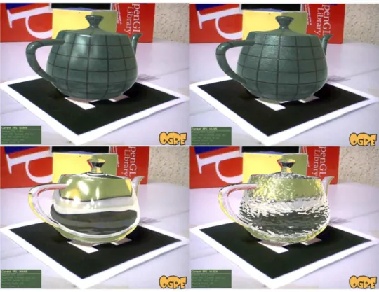
Figura 15: Scene generated by our method under typical lighting conditions.
to (Aittala 2010). When the marker is presented in a dark environment, the tracking produces more errors, but our method is still able to render with a coherent illumination in those circunstances, as we can observe in Figure 16. The augmented content reflects environmental lighting conditions, being illuminated by a cyan light, similar to the real world light originated from the computer screen. Also in Figure 16, we can observe that our method is able to handle the marker occlusions from the camera or from fingers.
Figura 16: Scene generated by our method under dark lighting conditions.
Figura 17: Scene generated by our method when the marker is illuminated by a flashlight.
7
Conclusion
This study presented a novel Augmented Reality pipeline with a photometric cali-bration stage. The existence of this stage enables signifficant realism improvement during the rendering of augmented content: we are able to mimic real world illumination when rendering augmented reality scenes.
This work contains two major contributions: a novel feature descriptor, faster than current state-of-the art methods with equivalent precision and half of memory usage, and; a novel on-the-fly photometric calibration method aware to lighting changes and without relying on light probes. The photometric calibration stage can be seamlessly integrated to current non fiducial tracking approaches by introducing a volumetric marker: a cuboid whose faces are textures. We also created a evaluation framework to measure the precision of our calibration. Our pipeline uses a custom redering engine that coupled with the feature descriptor are able to deliver fast rendering and tracking results: the bottleneck of our prototype was the camera capturing rate.
The illumination model used in our estimation contains only one directional light and an ambient component. We believe that this illumination model is enough to mimic lighting configuration of simple scenes, but may not generate convincent results in places with many local lights with different colors. Besides, our method presents the same marker limitations of non fiducial tracking approaches: the markers need to present good image features (high gradient value) to be nicely tracked. Our method is not able to consider local lighting variations in the same marker, like shadows. In other words, a shadow present in themarker will not be visible in the augmented content. But, its existence will influence the power of the light incident in the rendered model.
References
Agusanto et al. 2003 AGUSANTO, K. et al. Photorealistic rendering for augmented reality using environment illumination. In: Proceedings of the 2nd IEEE/ACM International Symposium on Mixed and Augmented Reality. Washington, DC, USA: IEEE Computer Society, 2003. (ISMAR ’03), p. 208–. ISBN 0-7695-2006-5. Disponível em: <http://dl.acm.org/citation.cfm?id=946248.946791>.
Aittala 2010 AITTALA, M. Inverse lighting and photorealistic rendering for augmented reality.Vis. Comput., Springer-Verlag New York, Inc., Secaucus, NJ, USA, v. 26, n. 6-8, p. 669–678, jun. 2010. ISSN 0178-2789. Disponível em:< http://dx.doi.org/10.1007/s00371-010-0501-7>.
Azuma 1997 AZUMA, R. T. A survey of augmented reality. Presence: Teleoperators and Virtual Environments, v. 6, n. 4, p. 355–385, ago. 1997.
Barandiaran et al. 2013 BARANDIARAN, I. et al. A new evaluation framework and image dataset for keypoint extraction and feature descriptor matching. 8th Int. Joint Conf. on Comp. Vis., Imag. and Comp. Graph. Theory and App. - VISAPP, p. 252–257, 2013.
Bastos e Dias 2005 BASTOS, R.; DIAS, J. M. S. Fully automated texture tracking based on natural features extraction and template matching. In:Proceedings of the 2005 ACM SIGCHI International Conference on Advances in computer entertainment technology. New York, NY, USA: ACM, 2005. (ACE ’05), p. 180–183. ISBN 1-59593-110-4.
Bauer, SÃijnderhauf e Protzel 2007 BAUER, J.; SÃijNDERHAUF, N.; PROTZEL, P. Comparing several implementations of two recently published feature detectors. In:Proc. International Conference on Intelligent and Autonomous Systems. [S.l.: s.n.], 2007.
Bay et al. 2008 BAY, H. et al. Speeded-up robust features (surf). Comput. Vis. Image Underst., Elsevier Science Inc., New York, NY, USA, v. 110, n. 3, p. 346–359, jun. 2008. ISSN 1077-3142.
Bo et al. 2011 BO, L. et al. Object recognition with hierarchical kernel descriptors. In: IEEE International Conference on Computer Vision and Pattern Recognition. [S.l.: s.n.], 2011.
Bradski e Kaehler 2008 BRADSKI, G.; KAEHLER, A. Learning OpenCV: Computer Vision with the OpenCV Library. 1st. ed. [S.l.]: O’Reilly Media, 2008.
Calonder et al. 2012 CALONDER, M. et al. BRIEF: Computing a local binary descriptor very fast.Pattern Analysis and Machine Intelligence, IEEE Transactions on, v. 34, n. 7, p. 1281 –1298, july 2012. ISSN 0162-8828.
Debevec 1998 DEBEVEC, P. Rendering synthetic objects into real scenes: bridging traditional and image-based graphics with global illumination and high dynamic range photography. In: Proceedings of the 25th annual conference on Computer graphics and interactive techniques. New York, NY, USA: ACM, 1998. (SIGGRAPH ’98), p. 189–198. ISBN 0-89791-999-8. Disponível em: <http://doi.acm.org/10.1145/280814.280864>. Debevec e Malik 1997 DEBEVEC, P. E.; MALIK, J. Recovering high dynamic range radiance maps from photographs. In: Proceedings of the 24th annual conference on Computer graphics and interactive techniques. New York, NY, USA: ACM Press/Addison-Wesley Publishing Co., 1997. (SIGGRAPH ’97), p. 369–378. ISBN 0-89791-896-7. Disponível em:<http://dx.doi.org/10.1145/258734.258884>.
Everingham 2006 EVERINGHAM, M. The Pascal Visual Ob-ject Classes (VOC) Challenge. In: . [s.n.], 2006. Disponível em:
<http://pascallin.ecs.soton.ac.uk/challenges/VOC/databases.html>.
Fischler e Bolles 1981 FISCHLER, M. A.; BOLLES, R. C. Random sample consensus: a paradigm for model fitting with applications to image analysis and automated cartography. Commun. ACM, ACM, New York, NY, USA, v. 24, p. 381–395, June 1981. ISSN 0001-0782.
Gadelha e Carvalho 2014 GADELHA, M.; CARVALHO, B. DRINK - Discrete Robust INvariant Keypoints. In: Pattern Recognition (ICPR), 2014 22nd International Conference on. [S.l.: s.n.], 2014. p. To be published.
Gomes, Carvalho e Gonçalves 2013 GOMES, R. B.; CARVALHO, B. M. de;
GONcALVES, L. M. G. Visual attention guided features selection with foveated images. Neurocomputing, v. 120, p. 34–44, 2013.
Gonzalez e Woods 2006 GONZALEZ, R. C.; WOODS, R. E. Digital Image Processing (3rd Edition). Upper Saddle River, NJ, USA: Prentice-Hall, Inc., 2006. ISBN 013168728X.
Gruber, Richter-Trummer e Schmalstieg 2012 GRUBER, L.; RICHTER-TRUMMER, T.; SCHMALSTIEG, D. Real-time photometric registration from arbitrary geometry. 2012 IEEE International Symposium on Mixed and Augmented Reality (ISMAR), IEEE Computer Society, Los Alamitos, CA, USA, v. 0, p. 119–128, 2012.
Harris e Stephens 1988 HARRIS, C.; STEPHENS, M. A combined corner and edge detector. In: In Proc. of Fourth Alvey Vision Conference. [S.l.: s.n.], 1988. p. 147–151.
He et al. 2009 HE, W. et al. Surf tracking. In: Computer Vision, 2009 IEEE 12th International Conference on. [S.l.: s.n.], 2009. p. 1586 –1592. ISSN 1550-5499.
Society, 2012. (ISMAR ’12), p. 91–97. ISBN 978-1-4673-4660-3. Disponível em:
<http://dx.doi.org/10.1109/ISMAR.2012.6402544>.
Ke e Sukthankar 2004 KE, Y.; SUKTHANKAR, R. PCA-SIFT: A more distinctive representation for local image descriptors. In: Proceedings of the 2004 IEEE Comp. Vis. and Patt. Rec. Washington, DC, USA: IEEE Computer Society, 2004. (CVPR’04), p. 506–513.
Klein e Murray 2008 KLEIN, G.; MURRAY, D. Improving the Agility of Keyframe-Based SLAM. [S.l.]: Springer Berlin Heidelberg, 2008. 802-815 p. (Lecture Notes in Computer Science, v. 5303). ISBN 978-3-540-88685-3.
Lee e Jung 2011 LEE, S.; JUNG, S. K. Estimation of illuminants for plausible lighting in augmented reality. In: ISUVR. IEEE, 2011. p. 17–20. ISBN 978-1-4577-0356-0. Disponível em: <http://dblp.uni-trier.de/db/conf/isuvr/isuvr2011.html>.
Leutenegger, Chli e Siegwart 2011 LEUTENEGGER, S.; CHLI, M.; SIEGWART, R. Y. Brisk: Binary robust invariant scalable keypoints. In: Proceedings of the 2011 International Conference on Computer Vision. Washington, DC, USA: IEEE Computer Society, 2011. (ICCV ’11), p. 2548–2555. ISBN 978-1-4577-1101-5.
Lourakis e Argyros 2004 LOURAKIS, M. I. A.; ARGYROS, A. A. Vision-based camera motion recovery for augmented reality. In: Proceedings of the Computer Graphics International. Washington, DC, USA: IEEE Computer Society, 2004. (CGI ’04), p. 569– 576. ISBN 0-7695-2171-1. Disponível em: <http://dx.doi.org/10.1109/CGI.2004.100>. Lowe 2004 LOWE, D. G. Distinctive image features from scale-invariant key-points. Int. J. Comput. Vision, Kluwer Academic Publishers, Hingham, MA, USA, v. 60, n. 2, p. 91–110, nov. 2004. ISSN 0920-5691. Disponível em:
<http://dx.doi.org/10.1023/B:VISI.0000029664.99615.94>.
Mair et al. 2010 MAIR, E. et al. Adaptive and generic corner detection based on the accelerated segment test. In: DANIILIDIS, K.; MARAGOS, P.; PARAGIOS, N. (Ed.). Computer Vision âĂŞ ECCV 2010. [S.l.]: Springer Berlin Heidelberg, 2010. (Lecture Notes in Computer Science, v. 6312), p. 183–196. ISBN 978-3-642-15551-2.
Malis e Vargas 2007 MALIS, E.; VARGAS, M. Deeper understanding of the homography decomposition for vision-based control. [S.l.], 2007. 90 p. Disponível em:
<http://hal.inria.fr/inria-00174036>.
Mikolajczyk e Schmid 2005 MIKOLAJCZYK, K.; SCHMID, C. A performance evaluation of local descriptors. Pattern Analysis and Machine Intelligence, IEEE Transactions on, v. 27, n. 10, p. 1615–1630, 2005. ISSN 0162-8828.
Miksik e Mikolajczyk 2012 MIKSIK, O.; MIKOLAJCZYK, K. Evaluation of local detectors and descriptors for fast feature matching. In: Pattern Recognition (ICPR), 2012 21st International Conference on. [S.l.: s.n.], 2012. p. 2681–2684. ISSN 1051-4651.