Mid-auction information acquisition

I

.

EPGE

FUNDAÇÃO GETULIO VARGAS

Escola de Pós-Graduação em Economia

Seminário de Almoço

"Mid-Auction Information Acquisition"

Leonardo Rezende

(Stanford University)

4

a

_{feira, dia 3 de janeiro às 12:30 horas}

EPGE, 10° andar, Sala 3

"Free lunch"

para alunos e professores: sanduíches, refrigerantes e

r

Mid-Auction Information Acquisition

Leonardo Rezende*

October 9, 2000

Abstract

This paper studies a model of a sequential auction where bidders are allowed to acquire further information about their valuations of the object in the middle of the auction. It is shown that, in any equilibrium where the distribution of the final price is atornless, a bid-der's best response has a simple characterization. In particular, the optimal information acquisition point is the same, regardless of the other bidders' actions. This makes it natural to focus on symmetric, undominated equilibria, as in the Vickrey auction. An existence theo-rem for such a class of equilibria is presented. The paper also presents some results and numerical simulations that compare this sequential auction with the one-shot auction. 8equential auctions typically yield more expected revenue for the seller than their one-shot counterparts. 80 the possibility of mid-auction information acquisition can provide an explanation for why sequential procedures are more often adopted.

1 Introduction

This paper studies a continuously ascending price independent private values auction, with the added richness that bidders are allowed to acquire further information about the value of the good in the middle of the auction. The information structure allows bidders to have different initial signals of their valuation and different privately known costs of acquiring information. The

framework can also accommodate for the possibility of some bidders already knowing their valuation at the outset of the auction or, conversely, not being able to acquire information with some probability.

It turns out that in some aspects the optimal strategy of a bidder in such an auction is quite simple. For example, the price at which information is acquired does not depend on the expected behavior of the other players. This greatly simplifies the characterization, numerical computation, and proving the existence of the equilibrium.

Why is it interesting to study models with mid-auction information acqui-sition? A direct reason is its potential application in complex environments, where a bidder participates in many different auctions, such as in simultane-ous ascending auctions or online auctions. In complex environments, gather-ing information and computgather-ing valuations for alI goods and combinations of goods can be an overwhelming task. It is not unreasonable to imagine that bidders approach the problem with just crude estimates of the valuations, and as the auctions proceed, they elect to concentrate their computational resources in evaluating the most promising alternatives. This paper is a first step towards modeling this behavior.

The current one good mo deI also offers an explanation on why sequential auctions seem to be so much more popular than their one-shot counterparts. Several explanations have been forwarded for this puzzle. Milgrom and We-ber (1982) have shown that under affiliation a sequential English auction generates more revenue than one-shot, sealed-bid rules. An English auction may also in practice be superior to a Vickrey auction because it is more immune to manipulation by the auctioneer.

However, affiliated models are hard to generalize to more complex set-tings, such as auctions of multiple goods. In such complex situations one issue that becomes important to the bidders is the cost of collecting informa-tion and processing it into bidding strategies. This suggests an alternative explanation for why sequential auctions might be useful: they allow bidders to revise their decisions in information acquisition in the middle of the auc-tions, and this option might be valuable not only to bidders but to the seller as well.

This model may also be helpful in econometric applications. Data in the "serious" tail of the bid distribution usually reflect much more accurately the valuations of the bidders than the rest of the distribution. Since the equilibrium of this mo deI also has this feature, the model may potentially be helpful in structural estimation of auctions.

Given the fundamental role that asymmetric information takes in Con-tract Theory and Mechanism Design, there has been surprisingly little work that treats the information acquisition process as endogenous. Some authors have studied information acquisition in the context of Baron-Myerson-style agency mo deIs (Crémer and Khali11992, Lewis and Sappington 1997, Crémer, Khalil, and Rochet 1998b, Crémer, Khalil, and Rochet 1998a).

Several authors have studied information acquisition in the context of auctions. In most cases, the analysis is restricted to ex-ante information acquisition, and to particular functional forms of the valuation and signal

distributions.1

Matthews (1984) and Persico (2000) study mo deIs where bidders can purchase information out of a continuum of alternative degrees of informa-tiveness. To do so, they resolve in different ways the non-trivial problem of

ranking distributions in terms of informativeness.2 _{Due to the simple}

struc-ture of the information acquisition problem that is imposed in this paper, this ranking is immediate here.

All papers cited in the last two paragraphs study situations where bidders are allowed to acquire information before the auction begins. Besides the already mentioned work Engelbrecht-Wiggans (1988), Iam not aware of any literature on information acquisition in sequential auction procedures.

The paper is structured as follows: Next section presents the setup that is used throughout the paper. The problem of characterizing the best re-sponse of a given bidder is then investigated. Section 4 contains a proof that an equilibrium of this game exists. Section 5 compares this equilibrium to what would arise in a one-shot game. In section 6 results of some numerical lExamples are Milgrom (1981b), Schweizer and von Ungern-Sternberg (1983), Lee

(1985), Hausch and Li (1993). Guzman and Kolstad (1997) study a setting similar to the one assumed here for one-shot procedures; however, these authors elect to characterize a rational expectations equilibrium in the spirit of Grossman and Stiglitz (1980), rather than use game-theoretical concepts.

simulations are presented.3

2 The Setup

I seek to investigate an auction mo deI that is conventional in all aspects, except for the mid-auction information acquisition decision.

All bidders are symmetric and have independent private valuations for the good to be auctioned. I represent these valuations by i.i.d. random variables

VI, ... ,V_{n ,} where n is the commonly known number of bidders. I assume

that the distribution function of Vi, Fv, is absolutely continuous with support

[O,

v].

The auction rules are also conventional: I mo deI a Japanese ascending

auction, where the price p begins at a low leveI (that I assume for simplicity

to be O) and increases continuously. Bidders should decide at which price to drop out. The auction ends when only one bidder is left, and he or she pays

the price at which the last of the other bidders dropped out. If alI remaining

bidders drop out at the same time, the winner is selected at random, with equal probability.

At any point in the auction each bidder can have two possible leveIs of

information about her own valuation. Each bidder initially has a signal Wi

about her valuation Vi, but can learn it perfectly and instantaneously at any

point in the auction at a cost Ci. Both Ci and Wi are known by player i in the

beginning of the game, but are not observed by anyone eIse. It is common

knowledge however that alI Wi are i.i.d. Fw, and likewise the Ci are Li.d. Fc. I

represent the distribution of Vi conditional on Wi by F_{v1w ,} and adopt a similar

notation for other conditional distribution functions. Except for

Wi

and

Vi,

all other variables are assumed to be independent.4

It is convenient to impose some further assumptions on the distributions

of Ci, Wi and Vi. I assume that they have bounded intervals as supportSj

the support of Vi is [O,

v]

and the one for Ci is [O,

e].

The support of Wi can

be anywhere, but I assume that the supremum of the support of

E[vilwil

is

strictly below

v.

I assume that eis high enough, so that there is always the

3The paper also contains an appendix that sketches a non-existence result for some distributional assumptions.

possibility that some bidder eIects not to acquire information. Also, I assume

that the distribution of Cj has an atom at O. Besides anaIyticaI convenience,

these assumptions allow me to accommodate in the same framework bidders that cannot acquire information and bidders that aIready have alI information at the outset of the auction.

Apart from the atom at O, alI distributions are assumed to have densities, and those are bounded above and away from zero everywhere in the support.

I assume that a higher Wi is good news about Vi, in the sense of Milgrom

(1981a); that is, if W

>

w',

then Fvl_w first-order stochastically dominates

Fv1wl .5

During the auction, the only information about the behavior of other players that a bidder observes is whether alI have dropped out or not, i.e., if the auction has ended or noto So I am ruling out both the possibility of observing early drop-out points or information acquisition points.

I conjecture that the assumption on the unobservability of drop-out points does not qualitatively affect the analysis (even though it greatly simplifies part of it). Notice that due to the IPV assumption, knowledge of other

player's drop-out pointjvaluation does not change i's estimate of her own Vi,

so a linkage effect as in Milgrom and Weber (1982) is not expected to existo The second assumption is possibIy not innocuous; direct observation of the information acquisition point can in principIe generate additional strate-gic effects that have not been accounted for in the present model.

3

The individual bidder's problem

I begin by studying the individual bidder's problem, taking as given the behavior of the other bidders. For notational simplicity I drop the subscript

i in this section and call Vi = V, etc.

It is convenient to summarize the other bidders' behavior in a reduced

form fashion. Let the random variable y represent the price at which the last

of the other bidders drops out.

Since y is a function of (Ci, W-i, V-i), it is initially independent of the

bidder's private information on Cj and Wi (and Vi, if she elects to acquire

information right from start). I will denote this distributions of y by Fy.

Under the unobservability assumptions made in the end of last section, no

information about y is obtained during the auction, except that y is greater than the current price. This alIows me to express the update of i's

informa-tion about y in a simple way. If bidder i were alIowed to observe the other

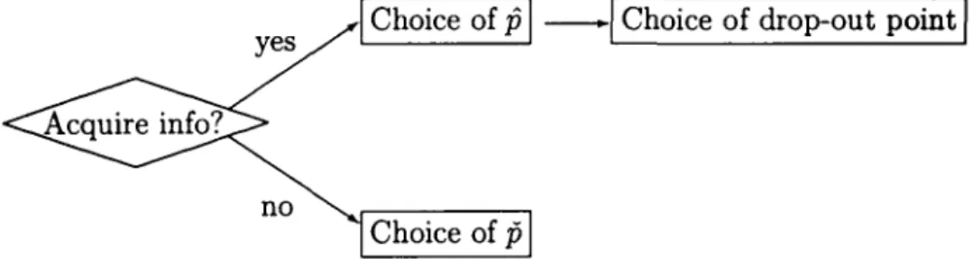
bidders' drop-out points, then the update formula would be more complexo The information acquisition process that has been imposed alIows me to separate the possible strategies of the bidder in two groups: either she

de-cides never to acquire information and drop out at a price

fi,

or she decides to

wait until a price fi and acquire information at this point.

fi

= O represents

immediate information acquisition, and

fi

=

00 represents never acquiring

information (or dropping out of the auction), so alI pure strategies are rep-resented by this parameterization. I consider in turn the optimal strategy within each grOUp, and later compare the two to find the overall optimal strategy.

yes

I

Choice of fi

I-I

Choice of drop-out point

I

no

Choice of

fi

Figure 1: Schematic representation of a bidder's strategy.

As will be seen in the equilibrium analysis in the next section, ones needs

to consider only the optimal response to the cases where Fy is absolutely

continuous. The appendix deals with the case where Fy contains jumps.

3.1 If the bidder decides to acquire information

The task in this section is to find the function

fi(

w, c, Fy ), defined as the

optimal information acquisition point for a bidder that observes a signal w

of her valuation, faces a cost c to acquire information, and expects that the other bidders behave in such a way that the highest price at which any oí

them stays in the auction is distributed according to y.

Define the function

U(p, q)

as the expected utility for a bidder that decides

to acquire information when the price reaches q, conditional on the price oí

conditional on w, c and Y 2: p. In a subgame perfect equilibrium fi should be

chosen as the q that maximizes this function at any given p.

After acquiring the information v, the bidder's dropping decision is

sim-pIe. It is dominant for her to drop out of the auction when p

2:

v and stay

otherwise. Throughout the paper I shall assume that this dominant strategy is always followed in this subgame.

Given that

U

for the region where p

>

q can be evaluated. In this region

the bidder would have dropped and incurred profit O if v ｾ＠ p, and otherwise

would expect to earn

E[v

-

ylv

>

y

>

p].6

80 defining

u(p,v)

E[v

-

ylv, v

>

y

> p] Pr[v >

ylv, y

> p]

{

_O ｊｰｕＨｶＭｹＩ､ｆｹｬｹｾｰＨｙＩ＠ ifv>p, _{if v ｾ＠ p,}

then

U(p, q)

=

E[u(p, v)lw]-

c, for all p

>

q.

It is convenient to rewrite this double integral as

for alI p

>

q, since from this expression it is easy to verify that

U

is difIeren-tiable with respect to p in this region, and its derivative obeys

a

A [A

1

00

] ｡ｰｕＨｰＬｱＩ］ｦｙｉｙｾｰＨｰＩ＠

U(p,q)+c- p (v-p)dFu1w(v) .

In the region where p

<

q, the bidder is staying in the auction without

knowing her v. Let f:l.p be an interval of time sufficiently small, so that still

p+ f:l.p

<

q. 8taying in the auction through this period, the bidders is subject

to one out of two outcomes: she may win the auction alone, if

y

E

(p, p+ f:l.p],

or the auction may continue, in which case she obtains an expected profit of

U(p

+

f:l.p, q).

80 we can write

Ｑ

ｰＫｾｰ＠

U(p, q)

=

p (E[vlw]- y)

､ｆｙｬｹｾ＠ + (1 - ｆｹｬｹｾｰＨｐ＠ +

f:l.p)) U(p

+

f:l.p, q),

for all p

<

p

+

b..p

<

q. Notice that independence was required to write the

expec!ation over v inside the integration signo Taking b..p -+ O, we conclude

that U is continuous with respect to p; rearranging and taking limits again

we obtain that

U

is differentiable with respect to p in this region as well, and

the derivative now obeys

8 -

[-

]

8p U(p, q)

=

fYIY?p(p) U(p, q) - E[v - plw] .

At p

=

q the function

U

is not necessarily differentiable, since its

left-and right-hleft-and derivatives exist but are generally different. It turns out that

by an application of the Envelope Theorem, the optimal fi is the point where

U

is differentiable with respect to p:

Proposition 1 Suppose eis not too large,1 i.e., c

<

v-E[vlw]. The optimal

fi(w, c, Fy ) is the point where the derivative of U with respect to p evaluated

at (fi, fi) exists, i. e., at the point fi uniquely determined by

Proof: We first notice that

U

is continuous with respect to q; it is constant

with respect to q in the region where p

> q

and depends on q only through the

boundary condition at p = q in the region where p

<

q. Also, any q

>

v

Ieads

to negative profits, that may be easily avoided by choosing q

=

o.

80 the

selection of the optimal information acquisition point may be circumscribed

to the compact interval [O,

v]

and by Weierstrass Theorem an optimum must

existo

We proceed by showing that at any interior point if the left- and

right-derivatives of

U

do not coincide, then this point cannot be an optimum.

8uppose that at q the right-derivative is smaller than the left-derivative.

Then there exists some E

>

O such that at p

<

q - E, U(p, q - E)

>

U(p, q).

80 it is suboptimal to wait until q.

Conversely, suppose now that the right-derivative is larger than the

left-derivative. Consider an E

>

O small enough so that, at alI points between

q and q

+

E,

this relation still holds. Then U(p, q

+

E)

>

U(p, q), for ali p

between q and q

+

E, and it would be suboptimal to acquire information at q.

Finally, notice that, at O, c> Joo(O - v) dFvl w, so the argument of the last

paragraph holds. Likewise, at fi the right-derivative is smaller, so this cannot

be an optimum either. 80 the optimum must be interior.

U niqueness of fi comes from the fact that J: (p - _{v) dFv1w} is a strictly

increasing function of p inside the support of Fv1w , since its derivative is

0+ J: dFv1w = Fv1w(p)

>

O. O

The optimality condition has a sensible economic interpretation: the cost of acquiring information, c, must be balanced against the benefit of doing so, namely, avoiding the potential loss from buying the good at a price higher than the bidder's valuation.

One remarkable feature about the condition that determines fi is that it

depends solely on the distribution of vlw; it does not depend on the specified

distributions for cor w, or on the behavior of the other players.

An immediate corollary is the following:

Corollary 1 lf c> O, then it is never optimal to acquire information at the

start of the auction.

80 positive information acquisition costs always have an impact on bidder

behavior, if this bidder plans to acquire information.

Let's investigate the properties of fi as a function of c and w. This is the

function obtained once one solves c

=

J:

(p -

_{v) dFv1w} for p. fi is an increasing

function of c (since its derivative with respect to c, by the implicit function theorem, is 1/ FVlw(fi(c, w))

2:

O).

As for w, notice that from the assumption that a higher w is good news

about v, for a fixed p the term J:(v - _p)dFvlw

=

Jmin{v - _p,0}dFv1w is

increasing in w, since the integrand is a weakly increasing function. 80 with

a higher w one needs a higher fi to reduce that termo

We conclude that fi is an increasing function of both c and w, and does

not depend on the behavior of the other players.

3.2 If the bidder decides not to acquire information

This case can be handled in an analogous fashion, defining

U(p,

r) as the

expected utility at p of a bidder that will drop out at r. Let

fi

be the optimal

droJrout point, given that the bidder does not acquire information.

U(p,

r)

=

O at the region where

p

> r, since then the bidder would

equation that

U

obeys before the information is acquired, since the bidder's situation is the same in both instances:

& • [ • ]

&p U(p,

r)

= !YIY?P(P) U(p,

r) -

E[v - plw] .

Also, as before, the chosen

p

will be such that the Ú is differentiable

at (P,P). 80 we have O =

ｾｕＨｐＬｐＩ＠

= !YIY?p(P) [O - E[v - Plw]]' or simply

P = E[vlw]. This is expected: this is simply the dominant strategy for a

player that could not acquire information in the first place, staying in the

auction until her expected valuation is reached.

3.3 The overall optimal response

In order to obtain the optimal response, one compares the payoff of the bidder

under each of the two alternatives discussed above. 8ince before both

p

and

p

the functions

U

and Ú follow the same differential equation, this comparison

can be made at any point p ｾ＠ min{p,p}.

A convenient comparison point is p

=

O, since at this point it is easy

to directly obtain expressions for Ú and

U:

they are simply the

(uncondi-tional) expected payoffs for a bidder at the outset of the auction under each alternative.

A bidder that elects not to acquire information and drops at P = E[vlw]

wins if y

<

P,

and gets v - y, and looses (and gains O) otherwise. 80 she has

an expected payoff of

while a bidder that plans to acquire information at

p

wins the auction if

y

<

por if

p

<

y

<

v, and incurs cost c if

y

>

p.

Her payoff is then

U(O,p)

=

1

15

1

OO

(v -

y)dFvlwdFy

+

loo

1

00 (v -

_{y) dFvlw dFy}

-

c(l -

Fy(p)).

3.3.1 Information acquisition as an option trade

It is convenient to rewrite the information acquisition decision in the following

fashion:

U(O,p) - U(O,P)

i

OO

(p - y)dFy

+

i

oo

[l

Y

(y - v) dFv1w -

c]

dFy

-J

max{y -

p,

O}dFy

+

J

max

{l

Y

(Y - v) dFv1w - c,

O}

dFy

J

r(t, c, w)dFy(t),

where r(t, c, w)

=

max{J; Fv1w(s)ds - c,

O} -

max{t -

p,

O}.

So the decision of acquiring information looks like the decision of trading

options on the underlying asset y; J rdFy is the expected profit from selling a

call option on y at strike price

p

and buying a call option on ｊｾ＠ Fv1w(s)ds - c

at strike price

p.

Figure 2 shows the shape of this r function. It is an

asymmetric spread, that pays if y is dose to

p,

has negative value if y is

too high, and O if y is too low. This suggests that information acquisition

depends negatively on the variance of y with respect to

vlw.

3.3.2 Comparative statics on the information acquisition decision

In the (c, w)-space, there will be a region A where condition U(O, p)

>

U(O,P)

is satisfied. In order to investigate the properties of the region A, we need

comparative statics results about the effect of c and w on

U

and

U,

and, to

do so, again we invoke the Envelope Theorem.

Observe that U(O, p) is the value function of a problem with c and w as

parameters, and where pis chosen to maximize U(O,

q),

with respect to

q.

The

Envelope Theorem8 _{then yields that lcU(O,p(c, w))}

₌

_-(1-

_{Fy(fi(c, w))}

_<

_O,

and of course lcU(O,p)

=

O. We condude that A shrinks as c increases.9

8Notice that the conditions for the Envelope Theorem are satisfied:

U

o is differentiable with respect to c and this derivative is continuous; and the solution <jJ(c, w) is unique (Milgrom 1999, Corollary 2).

0.06 ＬＭＭＭＭＭＭＭＮＭＭＭＭＭＭＭＬｲＭＭＭＬＭＭＭＭＭｲＭＭＮＮＬＭＭｾＭＭＬＮ｟Ｍ｟｟｟｟ｲＭＭＮＮＬＮ｟Ｍ｟｟｟Ｌ＠

0.05

0.04

0.03

0.02

0.01

ｯｾＭＭＭＭＭＭＭＭＭＭＭＭＭＭｾ＠

-0.01

To assess the effect of w we again invoke the Envelope Theorem to

dis-regard the effect through fi or fi, and use the assumption that higher w's are

good news.

Both v -y and max{ v-v,

O}

are increasing functions of v; so the integrals

with respect to vlw that appear in both expressions increase with w. We

conclude that 0(0, fi) and U(O, fi) both increase with w.

In the case where fi

<

fi, the sign of effect will depend on the comparison

of the effect of w on two integrals of v - _{y: J]5oo Jy}oo (v - y)dFv1wdFy versus

t

Jooo(v - y)dFvlwdFy. The impact of a larger w on both terms is positive.

If

the effect on the latter expression is larger than on the former, A shrinks

with w, and vice-versa.

One does not need to investigate the other case, where fi

>

fi, because of

the following result:

Proposition 2 For any type that strictly prefers to acquire information, fi

<

fi·

Proof: The strategy of the proof is to establish that if fi ｾ＠ fi, then U(O, fi)

-U(O,fi) ｾ＠ O. We start by noticing that, using equation 1, U(O, fi) - U(O,p)

=

J: Jooo (v - y) dFv1w dFy

+

J]5oo Jyoo (v - y) dFv1w dFy

+

J]5oo Jt (v - fi) dFvlw dFy.

If

fi

>

fi = E[vlw]' the first term is non-positive. 80 it remains to show

that the third negative term dominates the second. For any y

>

fi, of course

J;(Y - _{fi) dFv1w}

ｾ＠

°

and J;(v - _{fi) dFv1w}

ｾ＠

o.

80 Jyoo(v - _{y) dFv1w}

+

fo(v-fi) dFvlw

ｾ＠

Jyoo (v - fi) dFvlw

+

Jt (v - fi) dFv1w

ｾ＠

Jooo ( v - fi) dFv1w

=

fi - fi

ｾ＠

o.

80 the second and third terms are the integral of a non-positive integrando

O

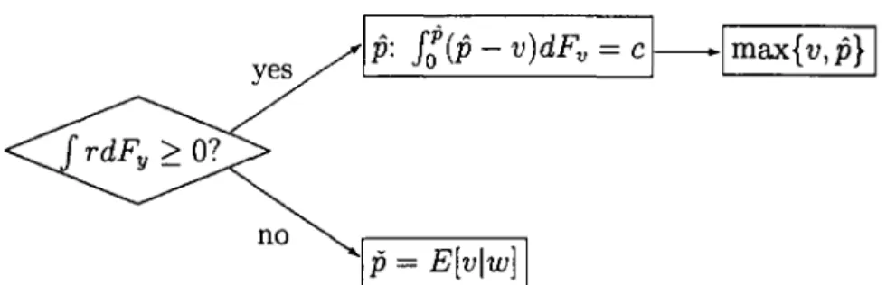
We collect the conclusions about a bidder's best response in the following

Proposition 3 Suppose that the other bidders act in such a way that the

highest drop-out point among them is an absolutely continuous random vari-able with distribution Fy. Then the best response to it by a bidder with type

(c, w) is as follows: lf J r(t, c, w)dFy

>

O, stay in the auction until the price

reaches fi; then acquire information, drop out if v ｾ＠ fi and othenuise drop

out when the price reaches v. lf J r(t, c, w)dFy

<

0, do not acquire

infor-mation and drop out at

fi.

Here

fi

=

E[vlw]' fi the unique solution to c

=

yes

no

_Ip

=

E[vlw]

I

Figure 3: 8chematic representation of an optimal strategy.

4 Equilibrium

From Proposition 3, we know that the distribution of the drop-out point of

a bidder that folIows the strategy described there is a mixture of max{p,

v}

and

p.

80 the distribution of Yi and, Iikewise, y, inherits the smoothness

properties imposed on the distributions of c, v and w.

To obtain an existence resuIt, it remains to verify that there exists a

distribution Fy such that a best response to it generates itseIf. This is done

in the next subsection.

4.1 Existence

Let F be the set of alI absolutely continuous distributions over [O,

ti]

and

A

the colIection of alI measurabIe subsets of types (c, w).

Define two appIications between these spaces. T: A -+ F gives the

distribution of Yi that would arise if a bidder was acquiring information if

her type was in

A;

i.e.,

T(A)(x) Pr[A] Pr[max{p, v} ｾ＠ xlA]

+

(1 - Pr[A]) Pr[p ｾ＠ xIAC ]

- r

_lA

Pr[max{p,

v}

ｾ＠

xlc,

w]dFc,w

+

_lAc

r

Pr[p

ｾ＠

xlc,

w]dFc,w

Notice that T(A) E F, since it is a mixture of absolutely continuous

distri-butions. Let F be the closure of F under the sup norm.lO

Define

R

:

F

-+

A

as folIows:

R(F)

= {

(c, w)

I

J

r(t, c, w)dFn-l(t)

ｾ＠

O } ,

ＭＭＭＭＭＭＭＭＭＭＭＭＭＭＭＭｾｾＭＭ

where r(t, c,

w)

=

ｭ｡ｸｻｊｾ＠ Fvlw(s)ds - c, O} - max{t -

E[vlw]'

O}. For an absolutely continuous distribution, this application selects the best response

A to it. Notice that, since any distribution function is of finite variation

and r is continuous with respect to y, the integral

J

rdFn-l is well

de-fined (Natanson 1961, Ch. 8, §6, Thm. 1), and for a sequence

Fk

-+

F,

1imk-+oo

J

rdFr-1

=

J

rdFn-1_{, by Helly's Second Theorem (Natanson 1961,}

Ch. 8, §7, Thm. 3).

Using this notation, the last object that we need to find to obtain a

symmetric equilibrium is a distribution F* E

:F

such that the information

acquisition decisions consistent with it generate it; that is, we need to find a fixed point

F* = T(R(F*)).

I will prove existence of an equilibrium applying the Schauder Fixed Point Theorem. To do so, I begin with some definitions from Topology.

A set is relatively compact if it is a subset of a compact set. A continuous

application is a compact map if its image is relatively compacto I recall the

following important result:

Theorem 1 (Ascoli-Arzelà) Let X be a compact metric space. lf S C

C(X) is equicontinuous and bounded, then S is relatively compact.

It is convenient at this point to impose bounds in the densities of w, C

and v:

Assumption 1 (Density Bounds) Assume the distributions of w and v

are absolutely continuous; the distribution of c is absolutely continuous,

ex-cept possibly for an atom 7r at O; and there are positive constants Mc, Mw,

Mv, and m such that fw ｾ＠ Mw, fv ｾ＠ Mv,

a:

(E[vlw])

2:

11m,

and fc(t) ｾ＠

Mc,Vt

>

O.

From the Ascoli-Arzelà Theorem, we obtain that

Proposition 4 T(A) is relatively compacto

Proof: Take X = [O,

v]

and S = T(A) in the Ascoli-Arzelà Theorem

Take

E>

O. Let 5

<

E/[(n-1)(Me+Mv+Mw/m)]. Let F be a distribution

in T(A).

So, for any x E [O,

ti],

one can write O :::; F(x

+

5) - F(x)

=

Pr[Yl E

[x, x

+

5]] :::; Pr[v E [x, x

+

5]]

+

Pr[p E [x, x

+

5]]

+

Pr[p E [x, x

+

5]].

We next observe that, using the Jacobian rule and the definition of

p,

we have that fp(s)

=

J

FVlw(s)fe

Uo

s Fv1w(t)dt) fw(w)dw. Since fe :::; Me and

Fv1w :::; 1, we obtain fp :::; Me. Also, fp

=

ＨｾＨｅ｛ｶｬｷ｝Ｉｲｬ＠

fw :::; Mw/m. It

then follows that, for sufliciently small 5,

As for the case where x = O, notice that v ｾ＠ p(O, w) = O. So the atom

in the p distribution is irrelevant, since we can write O :::; F(5) - F(O) :::;

Pr[v E [x, x

+

5]]

+

Pr[p E [x, x

+

5]]

<

(Mv

+

Mw/m)5

<

E. So T(A) is

equicontinuous. O

We now need to investigate continuity of the T o R operator.

Proposition 5 lf F E :F is such that Pr{J rdFn-l} is zero, then

T

o

R is

continuous at F.

Proof:

Take Ft -t F uniformly. Then, by Helly's Second Theorem,

J

rdF';'-l -t

J

rdFn-l. We can write

To R(F)(x) =

J

ｮｻｰｾｸｽ＠

+

ｮｻｦｲ､ｆｮＭｬｾｏｽＨｐｲ｛ｭ｡ｸｻｰＬ＠

v} :::; xlc, w] -

ｮｻｰｾｸｽＩ､ｆｻ｣ＬｷｽＡ＠

where

nO

denotes the indicator function. Applying Cauchy-Schwarz and the

(T o R(Fk)(X) - To R(F)(x))2 =

(J

Ｈｬｉｻｦｲ､ｆ［Ｍｬｾｏｽ＠

ＭＱｉｻｦｲ､ｆｮＭｬｾｯｽＩＨｐｲ｛ｭ｡ｸｻｰＬ＠

v}

ｾ＠

xlc,

ｗ｝ＭｉｉￜＧｾｘｽＩ､ｆＨ｣ＬｗＩＩ＠

2

ｾ＠

J

Ｈｬｉｻｦｲ､ｆ［Ｍｬｾｏｽ＠

ＭＱｉｻｦｲ､ｆｮＭｬｾｯｽＩＲ､ｆＨ｣ＬｷＩ＠

X

J

(Pr[max{p,

V}

ｾ＠

xlc,

W]

ＭｉｉￜＬｾｸｽＩＲ､ｆＨ｣ＬｷＩ＠

ｾ＠

J

Ｈｬｉｻｦｲ､ｆ［Ｍｬｾｏｽ＠

ＭＱｉｻｦｲ､ｆｮＭｬｾｯｽＩＲＮ＠

For any point outside {(c, w)

I

J

rdFn-l

=

O}, ｬｉｻｦｲ､ｆ［Ｍｬｾｏｽ＠ converges

pointwise to ｬｉｻｦｲ､ｆ［ＭｬｾｏｽＧ＠ So the limit of the integral of the last expression is

of a function that is zero almost everywhere. AIso, since the last expression

does not depend on x, convergence is uniform and continuity is established.

O

So existence would be guaranteed, if one could only restrict the analysis

to distributions where Pr[{ c, w

I

J

rdFn-l}]

=

O. Unfortunately, this is not

necessarily true for distributions that concentrate mass in low values: Since

r

=

O for sufficiently low values of y (see Figure 2), against these distributions

a positive mass of types will be indifferent about acquiring or not information

and proposition 5 cannot be applied.

It is not hard to impose assumptions that avoid this technical problem.

For example, suppose that with some positive probability 7l' bidders start the

game already knowing v. This is the same as assuming that there is an atom

7l' in the distribution of c at O, since bidders that start knowing v behave in

exactly the same way as bidders with zero cost.

This assumption is sufficient for existence; to see that, define, for 7l'

>

O

F7r

=

{(1-7l')F+7l'Fv

I

F E F}, where Fv is the (unconditional) distribution

of V. The next propositions show that we can restrict our attention to this

set.

Proposition 6 Suppose Pr[c = O] = 7l'

>

O. Then To R(F) C

F7r'

Proof: Notice that r(y, O, w)

2':

O. So, since we are resolving any indifference

that all types with c

=

o

are in A). AIso, p(O, w)

=

O. So for such A,

separating the types where c

=

O, we obtain

T(A)(x)

=

r

IT{p$x}dFe,w

+

r

Pr[max{p,

v}

:::;

xlc,

w]dFe,w

J ACn{e>O} J An{e>O}

+

r

Pr[maxp, v :::;

xlc,

w]dFe,w

J{e=o}

(1 - 7r)

[r

IT{p$x}dFe1e>o,w

+

r

Pr[max{p,

v}

:::;

xlc,

W]dFe1e>o,w]

J Nn{e>O} J An{e>O}

+

7r

r

Pr[v :::; xlw]dFe,w

J{e=o}

(1 - 7r)F(x)

+

7r

J

FVlw(x)dFw = (1 - 7r)F(x)

+

7rFv(x),

by the law of iterated expectations. Here F is the distribution defined as the

term between square brackets.

o

Proposition 7 For 7r

>

O, T o R is continuous in Frr.

Proof: From proposition 5, it is enough to verify that the measure of

{J

rdFn-l

=

O} is zero. From the Envelope Theorem, te

J

rdFn-l

=

1

-Fn-l(p). But for alI distributions in Frr, and any x

<

v,

F(x)

<

1-7rFv(x)

<

1. So

J

rdFn-l is strictly increasing in c everywhere, and for each w, there

is at most one c

>

O such that (c, w) E

{J

rdFn-l

=

O}. Furthermore,

this c can never be zero, because if F is in Frr, there is a positive

proba-bility of Yi occurring in any interval in the support

[O,

v].

So the integral

J

r(t, O, w)dFn-l is positive for these types. O

Now the fixed point resuIt comes from appIying the following

Theorem 2 (Schauder Fixed Point Theorem) Let C be a closed,

con-vex subset of a normed linear space and let h : C -t C be a compact map.

Then h has a fixed point.

Then we can finally state that

Proof: After proposition 3, it only remains to show that there exists a fixed

point to the

T

o

R

map in

F.

The set

F7r

is convex and closed. By propositions 4 and 7, the restriction

of

T

o

R

on

F7r

is a compact map, and by Proposition 6 its image is in

F1r'

80 8chauder's Theorem applies, and a fixed point F* exists in

F7r'

But F*

is in the image of

T

o

R,

so it also belongs to

F.

O

5 Comparison with the One-shot Auction

One virtue of the present analysis of the sequential auction is that it easily accommodates the case of a one-shot, Vickrey auction.

In a Vickrey auction, the bidders can act exactly as they would in the sequential auction, except that is not feasible anymore to acquire information in the middle of the auction. 80 a mo deI of this auction is the same as the

one studied so far, with the added restriction that

fi

= O.

8uppose this restriction is added to the individual bidder's best response

problem. Define

U

and

O

as before. The optimal

fi

is still

E[vlw]'

but now

the "maximization" of

O

forcefully leads to fi

=

O. The decision to acquire

information will still depend on the comparison of two quantities, 0(0,

O)

versus U(O,

fi).

Again, we can write 0(0, O) - U(O,

fi)

=

J

ro(t, c, w)dFJI(t),

where ro(t, c, w)

=

ｊｾ＠ Fvlw(s)ds - c - max{O, y -

p}.

This payofI difIerence is

also a combination of two options. Figure 2 shows how ro difIers from r.

Notice that the derivative of that integral with respect to c is 1, no matter

what Fy is expected to be.

Define, as before, Ro :

F

-+

A

as follows:

Ro(F)

= {

(c, w)

I

J

ro(t, c, w)dFn-1(t)

ｾ＠

O } ,

and To :

A

-+

F

as

To(A)(x)

=

r

Pr[v ::; xlc, w]dFc,w

+

r

Pr[p::; xlc, w]dFc,w.

lA

lAc

An equilibrium of the one-shot auction corresponds to a fixed point of

TooRo. Notice that the properties ofT and R described in propositions 4 and

for any distribution F E

F,

because

f

rodFn-l is always strictly increasing in c.lI

We conclude that

Proposition 9 An equilibrium ofthe one shot-auction exists (even if7r

=

O).

How do the equilibria of the two auctions compare? I have found out that, through numerical simulations, the distribution of the bids in the sequential auction frequently dominates the one in the one-shot auction. Because of that, one typically finds a higher expected revenue for the seller in the se-quential procedure.

In this section I formally show that, at least when n is large, the expected

revenue in the sequential auction is indeed higher. The numerical computa-tions presented in the next section show that this ranking can also be true

for n

=

2, so the conclusion of this result can be valid under more general

conditions.

As with the case of existence, I obtain the revenue comparison result through a series of propositions. I begin with a convenient definition:

Definition 1 A distribution F dominates C at the upper tail if there exists

some

x

<

v

such that F(x)

<

C(x) for ali x E

(x, v),

where vis the supremum

of the support of F.

The usefulness of this definition comes from the following proposition:

Proposition 10 lf F dominates C at the upper tail12 _{then, for sufficiently}

high n, the expected value of the rth-omer statistic of an i. i.d. sample of size

n from F is higher than the same expectation for C.

Proof: We first note that, after a change of variables, we can write this

expectation as B(n+1-r, r)-l foI F-1_(u)un-r_(1-uY-1_{du, and likewise for C,}

and where B is the Beta function (Arnold and Balakrishnan 1989, expression

2.1).

Therefore the difIerence in expected second-order statistics is proportional to foI [F-l(U) - C-1_(u)][un-r_{(1- uY-l]du. Let's look at the shape of each of}

the factors in square brackets to assess the sign of this expression.

llSee the proof of proposition 7 for the precise argument of why these ideas are related.

12 ... and F has a compact support [O, ü].

118!.IOH:GA MAHIU ｈｴｭｩＺｾｕｴＺ＠ ｓＡｍｕｎｓｾ＠

From the upper-tail dominance, there is a point

x

such that

F(x)

<

C(x),

for all

x

E

(x, v),

and

F(x)

ｾ＠

C(x),

for

x

E

(O,

x).

Let

ü

=

F(x);

then there is some set (ü, 1) such that

F-I

-

C-I> O there.

Now let's look at the behavior of

u

n - r

(1_uy-l.

Observe that, for

n

large

enough, it is increasing in (O,

ü),

and

ü

n - r

(1_üy-1

ｾ＠ O as

n

ｾ＠ 00. So we ean

bound the negative part ofthe integral, writing

IoÜ[F-I(

u)

-

C- I(u)]u

n - r

(1-uy-Idu

ｾ＠

ü

n - r

(1_ ÜY-I

IoÜ[F-I(U) -

C-I(u)]du

ｾ＠

-vüü

n - r

(1- üy-I

ｾ＠

O.

So for large enough n, the differenee beeomes positive. O

This is an useful result for revenue eomparisons, beeause expected rev-enues in auction mo deis are expeetations over seeond-order statistics, and also to efficieney eomparisons, being those related to eomparisons of mo-ments of first-order statistics.

How the distributions of drop-out points in the sequential and the one-shot auetion compare?

Proposition 11

For any F

E :F,

Ro(F)

C

R(F).

Proof: By inspeetion, r ｾ＠ ro. O

Proposition 12

For any A

E

A, T(A) jirst-order stochastically dominates

To(A).

Proof: Sinee Pr[max{p,

v}

:S

xlc, w]

-

Pr[v

:S

xlc, w]

:S

O, we obtain

T(A)(x)

-

To(A)(x)

=

IA

(Pr[max{p,

v}

::;

xlc, w]

-

Pr[v

:S

xlc, w]) dFc,w

:S

O. O

Proposition 13

Suppose that the supremum of the supporl of E[vlw]

(call

it ÜJ)

is

strictly below v. Then for any F, T(R(F)) dominates To(Ro(F)) at

the upper tail.

Proof:

T(R(F))

-

To(Ro(F))

=

T(R(F))(x)

-

To(R(F))(x)

+

To(R(F))

-To(Ro(F))

:S

To(R(F))

-

To(Ro(F)),

by proposition 12.

Substituting formulas we ean write that

To(R(F))(x)

-

To(Ro(F))(x)

=

IR\Ro (Pr[v

:S

xlc, w]

-

Pr[p

:S

xlc, w])dFc,w;

for any

x

E

(ÜJ, v),

Pr[p ::;

To see that the term is strietly negative, look at types with w close to iiJ

and low (but not zero) c. In the move from the one-shot to the sequential auetion, a positive mass of those types switehed their information acquisition

decision, sinee varies eontinuously with (at least) c. 80 R \ Ro has a positive

mass for high w-types. This means that Pr[v ::;

xlc,

w]

in a region with

positive mass, and the inequality is indeed striet. D

80 we eonclude that, holding the behavior of the opponents fixed, the

effeet of the ehange in the rules is an upper-tail dominanee for drop-out points of an individual bidder. This in turn implies a ranking in expected

revenue. AlI that remains is to obtain the result in equilibrium eomparisons,

as well. This is done through the folIowing result from Milgrom and Roberts (1994):

Theorem 3 Let 4>(x, t)

=

[4>dx, t), 4>H(X, t)] : [0,1] x T ｾ＠ [0,1], where T is

any partially ordered set. Suppose that, for all t E

T,

4> is continuous but for

upward jumps13 in x and that, for all x

E

[O,

1],

4> L and 4> H are monotone

nondecreasing in t. Then the set of fixed points of 4> is nondecreasing in t.

An application of this result to the problem at hand yields:

Proposition 14 For large enough n, the set expected revenues of all

sym-metric equilibria of the sequential auction is higher than the set of expected

revenues of the one-shot auction equilibria.

Proof: Take an appropriate closed, eonvex restriction of the domain of

T

o

R

such that it is eontinuous, like

:F

rr , and eonsider its image (that belangs in it,

by proposition 6). Aeeording to proposition 4, the closure of its image,

K,

is

eompact, is eonneeted and lies inside

:F

rr • Any fixed points wilI be in

K

as

welI, and we ean safely restrict attention to this set.

CalI the seeond-order expectation funetional J.L : K ｾ＠ [O,

'Ü],

J.L(F) =

B(n - 1,2)-1 foI F- 1(u)un -2(1 - u)du. For every F in K, by the previous

propositions we know there is a n*(F) so that, for n

>

n*(F), J.L(T(R(F)))

>

J.L(To(Ro(F))). Take an open balI around F so that this property still halds

inside it. Doing that for every F, we obtain an open covering of K. But

K is eompact; so there is a finite subeovering, and a maximal n*, such that

n

>

n* makes J.L(T(R(F)))

>

J.L(To(Ro(F))) for any F E K.

13Continuity but for upward jumps means that, for any x, limsuPxk)"x rPH(X/c, t) :5

Being K compact and connected, J1.(K) is a compact, connected set as well. It has to be a compact interval; call it

[a,

b].

Define the </J of Theorem 3 to be </J : [a, b] x {O, I} -+ [a, b], with </J(m, O)

=

J1. o To o

I4J

o J1.-1, and

</J(m, 1)

=

J1. o T o R o J1.-1.

Let's first verify that </J(m,

t)

is a compact interval, as required by Theo-rem 3. Since {m} is closed and J1. is continuous, J1. -1 (m) is a closed set within

a compact, and therefore is compacto It is also path-connected. 14 Its image

through the continuous application J1. o T o R is also connected and compacto

So </J(m,

t)

is a compact interval in [O,

v],

since these are the only connected sets on the line.

To verify continuity but for upward jumps, start with a sequence mie /"

m, and the corresponding sequence </JH(mk,

t).

Take a subsequence that

converges to lim sup </JH(mk, t). To each element of it there is a function

Fk in J1.-1(mk). This sequence of functions belong to a compact set, so it

has a subsequence that converges to a function F. Being J1. continuous,

J1.(F) = limJ1.(Fk) = m. So </JH(m,

t)

ｾ＠ limsup</JH(mk,

t).

The argument for the lim inf part is analogous. Applying Theorem 3 leads to the conclusion

that there are two sets, 10 and 11, such that (i) the expectations of equilibria

in the one-shot game are in 10 and those in the sequential auction are in 11,

(ii) inf 10 ｾ＠ inf 11 and

(iii)

sup 10 ｾ＠ sup!t.

This conclusion is not quite sufficient for our purposes because 10 and 11

may potentially be very large. There are many fixed points of </J that are

not equilibria: any distribution with the property that J1.(F)

=

J1.(T(R(F)))

would "look like" a fixed point from the point of view of </J.

To fix this important flaw, consider the family {</JkhE{0,1,2, ... } of corre-spondences defined as </Jk(m,

t)

= {min{b, J1.(Tt(Rt(F)) +k _IIF-To

(I4J

(F)) 11 x

IIF-T(R(F))II}

I

J1.(F)

=

m}. In this way </J0

=

</J, and for k

>

O we add to </J

k times the distance (in the sup norm) between F and each of the Tt(Rt(F))'s

(If

the result falls outside

[a,

b],

we just truncate).

Since all involved operations are continuous, alI the arguments done before for </J apply again for each </Jk, and we obtain sets

lt

and

lf

with properties (i), (ii) and (iii) as before. Consider

lá

= nk

lt

and

li

=

nk

lf.

These sets also have the same properties, and furthermore cannot contain any point that does not correspond to a true equilibrium expected revenue.

14This is because JJ is "linear" with respect to F-I; to see that, fix F and G in JJ-l(m) and for .À E [0,1], let H). be the function such that H-;1

=

.ÀF-1

+

(1 - .À)G-l. Then

To see that, fix m E It, m

<

b. For each k E {O, 1, 2, ... }, there is a Fk

with m

=

J.L(Fk)

=

J.L(Tt(Rt(Fk)))

+

kllF

k

- To(Ro(Fk))IIIIFk - T(R(Fk))1I .

This is a sequence in a compact; it has a subsequence converging to a

distribu-tion F and, by continuity, m = J.L(F) =

J.L(Tt(Rt(F)))+IIF-To(Ro(F))IIIIF-T(R(F))lllimk. The corresponding set of indices is exploding; so this

equa-tion can only be satisfied if

IIF -

To(Ro(F))11 = O or

IIF -

T(R(F))II = O. If

IIF-Tt(Rt(F))1I = O, then F is indeed a fixed point. If ｉｉｆＭｔｲＨｊｾｲｻｆＩＩＱｉ＠

=

0, for r =1=

t

only, then we have J.L(Tt{Rt{F)))

=

J.L(F)

=

J.L(Tr{Rt{F))), and this

contradicts proposition 13. O

6 Examples

This section discusses the computation for some choices of distributions for

c, w and v. The motivation for this exercise is twofold: first, it shows how

an equilibrium can be computed.15 _{Second, it establishes some}

quantita-tive meaning to the comparaquantita-tive statics finding that the sequential auction revenue-dominates the one-shot procedure.

As mentioned before, for alI examples simulated this revenue ranking holds for any number of bidders between 2 and 10. Numerical results also suggest that it might be true that in fact the distribution of drop-out points in the sequential auction in fact first-order stochastically dominates the one in the one-shot auction.

I begin by discussing the computational method.

6.1 Computational Method

To compute the equilibrium, I iterate until a fixed point is found, but instead

of working with the

F

space, I work on the

A

space; that is, I seek to find a

set A* of (c, w)-types such that A*

=

R o T(A*).

All expectations are calculated through a quasi-Monte Carlo method.

More specifically, 3 Weyl sequences with K elements have been drawn.16

15In particular, equilibria exist and are easy to compute also in conditions not covered by the existence theorem.

16_{The number of draws utilized so far has ranged from 3000 to 9000. This is admittedly}

Two of these sequences have been used to construct samples of

(c, w)-types,

and the corresponding

p

and

p

have been computed.17

Given a candidate set At, the algorithm computes the distribution of Yi

(the individual bidder drop-out point) that would arise if only types in At

acquired information. For each type, it is then computed what is the best

information acquisition decision against the highest order-statistic of y, and

this leads to a new At+1. The method then iterates until convergence.18

An advantage of this rather crude procedure is that the representation of

A is left free; I have tried before parameterizations for the border of A, 19 but

polynomials or splines did not seem to fit this function well.

A disadvantage is that of course the method need not necessarily converge.

My experience so far is that the distance Pr(At \ At+1 U At+1 \ At) goes down

quite fast in the first couple of iterations, so the initial guess does not seem

to be much important. 80 "almost" convergence is easy to achieve in most

cases. Literal convergence, that is, to drive the distance of At and At+l to

literally zero, sometimes is somewhat harder. 80 some loops may exist, but

the sets that loop seem to be dose to each other for the cases that have been studied so far.

6.2 Numerical Results

Here results for the case with

w

ｾ＠

U[O,

1] and c ｾ＠

U[O,

0.05] are considered.

I analyze three alternatives for the distribution of

vlw,

for

n

between 2 and

10.

The three alternatives for the distribution of

vlw

were

U[O, 2w], U[w, w+l]

and

U[w,

1]. The reason for these choices was to look at distributions where

the variance increases, stays constant, and decreases with w. This is of

interest because according to the discussion of section 3.3.1, the impact of

w through variance is a potentially important determinant of information

acquisition.20

17The last sequeoce is used to obtain a sample of

vlw

where oeeded.

18Notice that by focusing 00 symmetric equilibria and Yi rather than directly computing

a sample Y

=

max{Yl, ... ,Yn-l}, ooe cao avoid the curse of dimensiooality: lo the present algorithm the oumber of q-MC draws does oot depeod 00 n.

19Recall that, as loog as 1 - Fy(jJ) > 0, this border is the graph of a functioo c(w) in the (w, c)-plane.

2°Notice that these distributiooal assumptions violate several of the cooditions imposed

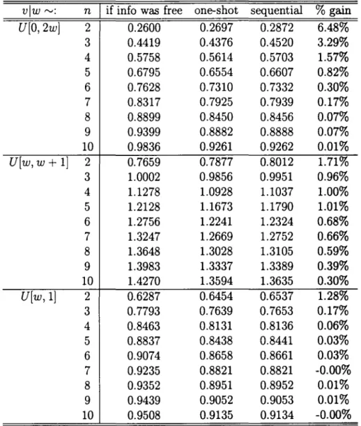
Besides computing equilibria for these 24 cases, I have also computed the equilibria of the corresponding one-shot auction in each case. This allowed me to calculate the expected revenue for the seller in each case.

Table 1 presents the computed expected revenue of the seller under each circumstance. In order to provide a benchmark, the first column shows what would be the revenue if information was costless to all bidders (Le., if every

bidder would drop out at V).21 The second and third columns show the

expected revenue in the one shot and the sequential auctions. Finally, the last column shows the percentage difference of revenue (in terms of the one-shot auction).

In percentage terms, the increased revenue of a sequential procedure

ranges from O to 6% - arguably, an economically significant figure. In

almost alI cases the gain is positive. A negative gain has been computed in the last specification for large values of n. It is not clear whether this is in fact true or it is due to the imprecision of the computation for high values of

n.

It is interesting to note that as n grows large, the gain becomes small,

both in absolute and percentage terms. This observation, coupled with the asymptotic comparison result, suggests that the expected revenue is generally higher with the sequential procedure.

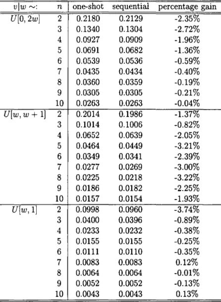
Table 2 shows the ex-ante expected payoff of an individual bidder under

each rule for alI settings, Le., the expected profit average over all

(c,

w)-types. In most cases the expected payoff under the sequential procedure is

lower than in the one-shot auction. 80 sequential auctions seem to benefit

the seller partially at the expense of the bidders.

Figures 4, 5 and 6 exhibit how the sets of types that acquire information (top panels) and the distributions of the individual drop-out points (bottom panels) are under each alternative. For convenience, only equilibria with

n

=

2 are depicted. Equilibria with more bidders have smaller information

acquisition regions, but the the shape of these regions and of the drop-out convenience, and are not necessary for existence or revenue rankings.

21 A counterintuitive finding is that 50metimes the sequential auction is more profitable than if information was for free. This can only occur however for n

=

2. The logic is the following: suppose c is extremely high, 50 that nobody effectively buys information. In this case the revenue is the expected value of the second order statistic of a sample of

E[vlwi]' rather than of Vi. With many bidders, the latter is larger than the former, but not

when the number ofbidders is 2: in this case, E[min{E[vlwl]' E[vlw2]}] > E[min{Vlt112}].

vlw

rv: n

I

if info was free one-shot sequential

%

gain

U[0,2w]

2 0.2600 0.2697 0.2872 6.48%

3 0.4419 0.4376 0.4520 3.29%

4 0.5758 0.5614 0.5703 1.57%

5 0.6795 0.6554 0.6607 0.82%

6 0.7628 0.7310 0.7332 0.30%

7 0.8317 0.7925 0.7939 0.17%

8 0.8899 0.8450 0.8456 0.07%

9 0.9399 0.8882 0.8888 0.07%

10 0.9836 0.9261 0.9262 0.01%

U[w,w+

1] 2 0.7659 0.7877 0.8012 1.71%

3 1.0002 0.9856 0.9951 0.96%

4 1.1278 1.0928 1.1037 1.00%

5 1.2128 1.1673 1.1790 1.01%

6 1.2756 1.2241 1.2324 0.68%

7 1.3247 1.2669 1.2752 0.66%

8 1.3648 1.3028 1.3105 0.59%

9 1.3983 1.3337 1.3389 0.39%

10 1.4270 1.3594 1.3635 0.30%

U[w,l]

2 0.6287 0.6454 0.6537 1.28%

3 0.7793 0.7639 0.7653 0.17%

4 0.8463 0.8131 0.8136 0.06%

5 0.8837 0.8438 0.8441 0.03%

6 0.9074 0.8658 0.8661 0.03%

7 0.9235 0.8821 0.8821 -0.00%

8 0.9352 0.8951 0.8952 0.01%

9 0.9439 0.9052 0.9053 0.01%

10 0.9508 0.9135 0.9134 -0.00%

vlw

r-v: n

I

one-shot sequential percentage gain U[0,2w] 2 0.2180 0.2129 -2.35%

3 0.1340 0.1304 -2.72%

4 0.0927 0.0909 -1.96%

5 0.0691 0.0682 -1.36%

6 0.0539 0.0536 -0.59%

7 0.0435 0.0434 -0.40%

8 0.0360 0.0359 -0.19%

9 0.0305 0.0305 -0.21%

10 0.0263 0.0263 -0.04%

U[w,w

+

1] 2 0.2014 0.1986 -1.37%

3 0.1014 0.1006 -0.82%

4 0.0652 0.0639 -2.05%

5 0.0464 0.0449 -3.21%

6 0.0349 0.0341 -2.39%

7 0.0277 0.0269 -3.00%

8 0.0225 0.0218 -3.22%

9 0.0186 0.0182 -2.25%

10 0.0157 0.0154 -1.93%

U[w,l] 2 0.0998 0.0960 -3.74%

3 0.0400 0.0396 -0.89%

4 0.0233 0.0232 -0.38%

5 0.0155 0.0155 -0.25%

6 0.0111 0.0110 -0.35%

7 0.0083 0.0083 0.12%

8 0.0064 0.0064 -0.01%

9 0.0052 0.0052 -0.13%

10 0.0043 0.0043 0.13%

distributions are qualitatively similar.

The lower panels show that typically the distribution of drop-out points

in the sequential auction almost dominates the one for the one-shot auction.22

The impact of the sequential rule can occur either at lower, intermediate or upper quantiles.

As top panels show, the information acquisition regions are indeed

mono-tonic in c, but not necessarily so in w. A more optimistic signal about the

good's valuation can make the bidder more (as in the first specification) or less (as in the second one) eager to acquire information, depending on how

this news affect the dispersion of her valuation vis-à-vis the auction price.

A

A ppendix: N on-existence in the

degener-ate case

This appendix shows that, if the set of types is degenerate, an equilibrium may not existo

Consider the best response to a distribution of y that is mixed, Le., has

an absolutely continuous component and a finite set of atoms. Define (; and

p

as before. I contend that, as long as an atom of y does not occur at

p,

this

is still the optimal information acquisition point.

The reason for that is that atoms at p

=I

P

do not fundamentally affect

the derivation of the differential equation characterization done before, once derivatives are appropriately replaced by discrete jumps.

Take an interval

[p,

p

+

dp). If no atom of y falIs in this interval for small

enough dp, the derivation done before is unchanged. There may however be

an atom at p. We can always take dp small enough so that there are no

atoms in (p, p

+

dp). In this case, it is still possible to write, say,

l

rH-dP

U(p, q)

=

P (E[v] - ｴＩ､ｆｹｬｹｾｰＨｴＩ＠

+

[1 -

ＨｆｹｬｹｾｰＨｐ＠

+

dp) - _{ｆｹｬｹｾＨｐＩＩ｝ｕＨｰ＠}

+

dp, q)

for p

+

dp

<

q. The only problem is that ｆｹｬｹｾｰＨｐ＠

+

dp) -+ ｆｹｬｹｾＨｐＫＩ＠

>

ｆｹｬｹｾＨｐＩＮ＠ 80 U is discontinuous at this point; but the discontinuity point