Todos os direitos reservados.
É proibida a reprodução parcial ou integral do conteúdo
deste documento por qualquer meio de distribuição, digital ou
impresso, sem a expressa autorização do
REAP ou de seu autor.
Econometrics of Ascending Auctions by Quantile
Regression
Nathalie Gimenes
Econometrics of Ascending Auctions by Quantile
Regression
Nathalie Gimenes
Nathalie Gimenes
Econometrics of Ascending Auctions by Quantile
Regression
Nathalie Gimenes
Department of Economics, University of S˜ao Paulo, Brazil.
Abstract
This paper suggests an identification and estimation approach based on quantile regression to recover the underlying distribution of bidders’ private values in ascend-ing auctions under the IPV paradigm. The quantile regression approach provides a flexible and convenient parametrization of the private values distribution, with an es-timation methodology easy to implement and with several specification tests. The quantile framework provides a new focus on the quantile level of the private values distribution, in particular the seller’s optimal screening level, which can be very use-ful for bidders and seller. An empirical application using data from the USFS timber auctions illustrates the methodology.
JEL: C14, D44, L70
Keywords: Private values; timber auctions; ascending auctions; seller expected revenue;
quantile regression identification; quantile regression estimation; quantile regression
specifi-cation testing.
I am grateful to Emmanuel Guerre for his insightful comments and suggestions. I would like to thank the
editor and three referees as well as Leonardo Rezende, Jo˜ao Santos Silva, Quang Vuong, Isabelle Perrigne,
Valentina Corradi, Martin Pesendorfer, Rafael Coutinho Lima, Frank Verboven and Geert Dhaene for helpful
discussions. I acknowledge the School of Economics and Finance at Queen Mary University of London for
1
Introduction
In an auction theoretical game, the bidders’ private value cumulative distribution function
(c.d.f.) is a key element for analysing the demand that a seller faces. Because it is required in
the computation of the seller’s expected payoff, its knowledge is crucial for policy
recommen-dation, as e.g. the optimal reservation price policy. The issue here is that bidders’ private
values are not observed, thereby their distribution function is unknown for the
econometri-cians and policy makers. The goal of this paper is to propose an identification and estimation
approach based on quantile regression to recover the private value conditional distribution
in ascending auctions.
In the past 20 years, several structural researches have proposed parametric and
nonpara-metric approaches to identify and estimate the latent distribution of private values. A first
wave of researchers has focused on parametric strategies. See Paarsch (1992) and Donald and
Paarsch (1993, 1996) for Maximum Likelihood (ML) estimation, Laffont, Ossard and Vuong
(1995) for simulated method of moments based on the revenue equivalence, Rezende (2008)
for semiparametric linear regression models and Li and Zheng (2009) for a semiparametric
Bayesian method in a model with endogenous entry and unobserved heterogeneity.
Nonparametric approaches for ascending auctions have been proposed in an attempt to
circumvent the misspecification bias of parametric ones. See Haile and Tamer (2003) for
independent private values (IPV) and Aradillas-Lopez, Gandhi and Quint (2013) for the
affiliated setup. Menzel and Morganti (2013) built their nonparametric estimation on order
statistics, which can be also viewed as sample quantiles. A few nonparametric approaches
built on quantiles have been developed for first-price sealed-bid auctions. Using the insight
in Haile, Hong and Shum (2003)1, Marmer and Shneyerov (2012) argue that a quantile
1
approach makes the estimation of the private value p.d.f. easier from a derivation of the
private value quantile function. On a different direction, Guerre and Sabbah (2012) propose
to estimate quantile function instead of p.d.f..
Although nonparametric approaches have the advantages of being flexible in analysing
the data at hand since no additional structure is imposed, it has some drawbacks as the
curse of dimensionality and the need to choose for a smoothing parameter. The curse of
dimensionality can be indeed a relevant estimation issue in view of important contributions
to the empirical auction literature such as Haile and Tamer (2003) and Aradillas-Lopez et al.
(2013), which consider, respectively, 5 and 6 explanatory variables for a sample size of a few
thousands at best. By contrast, the quantile regression model suggested in this paper can be
estimated with a parametric rate, independently of the dimension of the auction covariate,
and does not involve the choice of a smoothing parameter.
The quantile regression model offers a flexible parametric specification for conditional
quantiles since includes functional components that may be helpful to reduce the impact of
misspecification. Compared to the semiparametric regression approach of Rezende (2008),
quantile regression is computationally more difficult to perform but delivers an estimation
of the full private value distribution, as needed for instance to derive an optimal reservation
price. As a consequence, quantile regression is probably better suited for policy
recommen-dations than a simpler regression approach. In particular, the quantile regression approach
allows to highlight the screening level implied by the choice of a reservation price, a policy
characteristic that has been mostly ignored by previous empirical approaches.
The identification strategy developed in this paper is built under the IPV setup and
combines the nonparametric quantile approach in Marmer and Shneyerov (2012) and Guerre
and Sabbah (2012) with a parametric quantile regression specification. The approach focus
on ascending auctions, but can be easily extended to other types of auctions (see Gimenes and
Guerre (2014)). Ascending auctions are especially suitable for the identification of the private
value distribution under the IPV paradigm because the transaction price equals the
second-highest private value. As a result, the private value distribution can be nonparametrically
identified through the winning bids distribution, as well known from Athey and Haile (2002)2.
Based on data from the United States Forest Service (USFS) timber auctions, the empirical
application suggests reservation price policies that may lead to a low probability of selling
the good, especially when there is a sharp increase in the private value conditional quantiles.
This is motivated by a high heterogeneity among the bidder, which may incentive sellers to
screen bidders with low valuation from participating in the auction.
The paper is organized as follows. Section 2 describes the quantile and quantile
re-gression identification approaches for ascending auctions. Section 3 provides the estimation
methodology and asymptotic properties. Section 4 investigates the exclusion participation
restriction. Section 5 provides an empirical application of the methodology. Finally, section
6 concludes the paper.
2
Identification
A single and indivisible object with characteristics Z ∈ Rd is auctioned to N ≥ 2 bidders
through an ascending auction. The seller sets a reservation price Rprior to the auction that
is the minimum price that he would be willing to accept. Both the set of auction covariates
X = (1, Z) and the number of actual bidders N participating in the auction are common
knowledge. The object is sold to the highest bidder for the price of his last bid, provided
that it is at least as high as the reservation price R(X). Within the IPV paradigm, each
2
bidder i = 1, . . . , N is assumed to have a private value Vi for the auctioned good, which
is not observed by other bidders. The bidder only knows his own private value, but it is
common knowledge for bidders and sellers that private values have been identically and
independently drawn from a common c.d.f. FV (·|X) conditional upon X, or equivalently,
with a conditional quantile functionV (α|X),α∈[0,1], defined as
V (α|X) := inf{v :FV (v|X)≥α}. (2.1)
When the private value conditional distribution is absolutely continuous with a
probabil-ity densprobabil-ity function (p.d.f) fV (·|X) positive on its support [V (0|X), V (1|X)] ⊂ R+, as
considered from now on, V (α|X) is the reciprocal function FV−1(α|X).
By the Fundamental Theorem of Simulation, Ui = FV (Vi|X), which can be viewed as
the rank of a bidder with private value Vi in the population, is independent of X with a
uniform distribution over [0,1]. The IPV paradigm implies that the ranks Ui, i= 1, . . . , N,
are independent. In other words, the dependence between the private values Vi and the
auction covariatesX can be fully captured by the nonseparable model
Vi =V (Ui|X), Ui iid
∼ U[0,1] ⊥X. (2.2)
Therefore, bidders are identical up to the variable Ui, which represents the bidder ith’s
position in the private value distribution.
The quantile regression approach, developed by Koenker and Bassett (1978), restricts
the quantile representation (2.2) to a regression specification, such as
V (α|X) = Xγ(α)
=γ0(α) +Zγ1(α),
where γ0(α) is the quantile regression intercept and γ1(α) the quantile regression slopes.
Note that in (2.3), both the intercept and the slope quantile regression coefficients depend
upon the rank α of the bidder in the population. Therefore, changes in the conditioning
variables not only shift the location of the conditional distribution of V, but may also affect
its scale and shape. A shock on the covariate X may affect a bidder with a low rank α in
a different way than a bidder with a higher rank. A large discrepancy of the coefficients
across α indicates high heterogeneity3 among the bidders. As discussed later, taking into
consideration such heterogeneity among the bidders may have important implications for
both seller and bidders.
I now turn to the assumptions of the model. In the considered ascending auction, bidders
raise continuously their prices and drop out of the auction as the prices reach their valuation.
Assumption 1 The transaction price in an auction is the greater of the reservation price
and the second-highest bidder’s willingness to pay.
Assumption 1 is an assumption on equilibrium play. This assumption was also used in
Aradillas-Lopez et al. (2013) and, as noted in Athey and Haile (2002) and Bikhchandani,
Haile and Riley (2002), is compatible with the multiple equilibria generated by ascending
auctions. It is for instance the result of the dominant strategy equilibrium of a button
auction, which is a stylized version of an ascending auction. Haile and Tamer (2003) use
instead assumptions concerning bidder’s behaviour, which determine the joint distribution
of all bids.
The following three assumptions are required for the identification result.
3
Note that heterogeneity and asymmetry are two concepts that should not be confused. Here,
het-erogeneity is concerned with the variation of γ(α) across quantile levels α, while asymmetry implies that
Assumption 2 V (α|X) is strictly increasing and continuous on its support [V (0|X),
V (1|X)] for all X.
Assumption 3 The private value conditional quantiles has a linear quantile regression
spec-ification
V (α|X) =Xγ(α). (2.4)
Assumption 4 The auction specific variable, Z, has dimension d, with a compact support
in Z ⊂(0,+∞)d and a nonempty interior.
Assumption 2 and 3 deal with the quantiles of the bidders’ private value distribution.
As-sumption 2 is usual in the quantile regression literature, whereas AsAs-sumption 3 imposes
correct specification of the private value conditional quantiles. Assumption 4 concerns the
auction specific covariateX = (1, Z) and ensures that ifxγ1 =xγ2, for allx∈ X ={1} × Z,
thus γ1 =γ2.
Define
Ψ (t|N) =N tN−1−(N −1)tN. (2.5)
and let W(α|X, N) be the α-quantile of the winning bids conditional distribution given
(X, N). It follows from Athey and Haile (2002, equation (5)) that Ψ (FV (·|X)|N) is the
distribution of the second-highest private value, which by Assumption 1 is equal to the
winning bid. The next Lemma gives the cornerstone identification result of the quantile and
quantile regression approaches.
Lemma 1 Under IPV and assumptions 1 and 2, for each N and α∈[0,1],
1. [Probability of winning.] A bidder with private valueV (α|X) wins with probability
2. [Identification.] The private value quantile maps to the winning bid quantile through
V (α|X) = W(Ψ (α|N)|X, N), (2.6)
where Ψ (α|N) is defined in (2.5).
3. [Stability property.] If assumptions 3 and 4 also hold,
(i) There exists a vector of coefficients β(α|N) such that
W(α|X, N) = Xβ(α|N) ;
(ii) β(α|N) is uniquely defined and satisfies
β(Ψ (α|N)|N) =γ(α). (2.7)
Lemma 1-(1) shows that the rankαof a bidder in the population has a direct relationship
with his probability of winning so that estimating V (α|X) can be helpful for newcomers
that do not know the market or to benchmark a desired probability of winning the auction.
Lemma 1-(2) gives the nonparametric identification of the private value conditional quantile
through the observed winning bid conditional quantile function. Result (i) in Lemma 1-(3)
is a stability property of the quantile regression specification, which is a consequence of
Lemma 1-(2). Indeed, the latter shows that the winning bid quantile function admits the
same linear specification as postulated for the private values, but for a transformed quantile
level. Result (ii) in Lemma 1-(3) gives the identification result of the quantile regression
approach. It shows that the coefficientγ(·) of the private value conditional quantile function
but evaluated at a different quantile level Ψ (·|N). The proof of Lemma 1 can be found in
the supplemental material, which also groups the proof of all results stated in this paper.
2.1
Optimal Reservation Price
This section study the seller’s expected payoff under a quantile perspective. Consider a
binding reservation price set by the seller, i.e. R(X)∈ [V (0|X), V (1|X)]. The reservation
price thus plays the role of a screening level in the auction since bidders with V (αi|X) <
R(X) are prevented from participating in the game. Let αR(X) be the screening level in
the private value conditional distribution, i.e. αR(X) is such that R(X) = V (αR|X). It
thus represents the percentage of bidders in the population that are not participating in
the auction because of a low valuation. Note that the auctioned good will not be sold if
all the players have valuation below R(X), which implies that the probability of trading
is 1 −αR(X)N. Therefore, for a given N, the probability of trading decreases with the
screening level αR(X).
Let the seller’s payoff be defined as
π(r) =WI(W ≥r) +V0(1−I(W ≥r)), (2.8)
whereW is the winning bid,V0 the seller’s private value andI(A) an indicator function equal
to 1 if the event Aholds and 0 otherwise. The following proposition gives a quantile version
for the seller’s expected payoff, a candidate for the optimal screening level α∗
R(X, V0) =
α∗
R(X, V0(X)) and for the corresponding optimal reservation price R∗(X, V0) = V (α∗R|X).
Let Π (α|X, N, V0) be the seller’s expected payoff given (X, N, V0) when the screening level
is α.
(i) The seller’s expected payoff is, for a screening level α,
Π (α|X, N, V0) = V0(X)αN +R(X)N αN−1(1−α)
+N(N −1)
Z 1
α
V (t|X)tN−2(1
−t)dt,
(2.9)
where V0(X) is the seller’s private value and R(X) the reservation price;
(ii) The optimal reservation price R∗(X, V0) = V (α∗
R|X) satisfies
R∗(X, V0)−V(1)(α∗R|X) (1−α∗R(X)) =V0(X), (2.10)
where V(1)(α|X) =∂V (α|X)/∂α is the private value quantile density function.
Proposition 2 is a quantile version of a standard result in the auction literature, see Riley
and Samuelson (1981, Proposition 1 and 3), Krishna (2010, p.23) and Myerson (1981). Note
that sinceV(1)(·|X)>0, it is clear thatα∗
R(X)> α0(X), whereV0(X) =V (α0|X). As well
known, the optimal reservation price policy does not depend upon the number of bidders.
3
Estimation Methodology
Consider L i.i.d. ascending auctions (Wℓ, Zℓ, ℓ= 1, . . . , L). Let Xℓ = (1, Zℓ) ∈ X be a row
vector of dimension d+ 1. The following assumption concerns the variables in our model:
Assumption 5 The variables{Nℓ, Xℓ, Viℓ, i= 1,2, . . . Nℓ, ℓ= 1, . . . , L}are independent and
identically distributed. The support[V (0|Xℓ), V (1|Xℓ)]⊂R+ ofViℓis bounded. Conditional
on Xℓ, the private values Viℓ are independent with common c.d.f. FV (·|Xℓ) and a density
Assumption 5 implies that each auction is independent and that, within an auction, the IPV
paradigm holds.
A standard approach in quantile regression interprets the coefficient β(α|N) in Lemma
1-(3) as the minimizer
β(α|N) = arg min
β∈Rd+1E[ρα(W −Xβ)|N],
where ρα(u) = u(α−I(u <0)). From (2.7), the unconditional γ(α) is also the minimizer
of the average across N
γ(α) = arg min
γ∈Rd+1E
ρΨ(α|N)(W −Xβ)
,
which suggests the estimator
b
γ(α) = arg min
γ∈Rd+1Qb(γ|α) whereQb(γ|α) =
1
L L
X
ℓ=1
ρΨ(α|Nℓ)(Wℓ−Xℓγ). (3.11)
The private value conditional quantile can be estimated via Vb(·|X) = Xbγ(·) and then
used into equation (2.9) to estimate the seller’s expected payoff Π (·|X, N, V0). Although
equation (2.10) in Proposition 2 gives a closed form to estimate the optimal reservation
price R∗(X, V0), it involves an estimation of the quantile density function V(1)(·|X). It is,
therefore, more convenient to estimateR∗(X, V0) as in Li, Perrigne and Vuong (2003) based
upon a maximization of the estimated expected payoff. This approach differs from Li et al.
(2003) in the sense that the expected payoff depends upon the quantile level and for this
reason it involves first an estimation of the optimal screening level.
are
b
Π (α|X, N, V0) = V0(X)αN+X′bγτL(α)N α
N−1(1−α) +N(N −1)Z 1
α
tN−2(1−t)X′bγτLdt,
b
αR(X, V0) = arg max
α∈[0,1]Π (b α|X, N, V0),
b
R(X, V0) = X′bγτL(αbR(X, V0)).
where τL in (0,1) is a sequence that goes to 0 when Lgrows and bγτ(·) is
b
γτ(α) =
b
γ(τ) for α in [0, τ),
b
γ(α) for α in [τ,1−τ],
b
γ(1−τ) for α in (1−τ,1].
This redefinition of the estimated quantile regression slope ensures existence for extreme
quantile levels near 0 and 1, provided τL is going to 0 slowly enough. Indeed, as seen from
Bassett and Koenker (1982, fig. 2), the standard estimator of the extreme quantile regression
slope coefficients are not unique and selecting some may give inconsistent estimators. An
standard solution is to define them as limits when quantile levels go to 0 or 1 as performed in
Bassett (1988) and studied in Chernozhukov (2005). The next Proposition gives conditions
for consistency of this estimation approach.
Proposition 3 Suppose that Assumptions 1-5 hold and that the population optimal screening
level is unique. Then, if τL goes to 0 slowly enough, αbR(X, V0) and Rb(X, V0) are consistent
estimators of the optimal screening level and reserve price.
Following Chernozhukov (2005), it is expected that Proposition 3 applies as soon as LτL is
supple-mental material.
3.1
Asymptotic Properties of the Estimator
In this section, the asymptotic properties4 of the private value quantile regression estimator
(3.11) are studied. In what follows, let Q(γ|α) = EhQb(γ|α)i and
b
Q(γb|α) =Qb(bγ(α)|α) = min
γ∈Rd+1
b Q(γ|α)
be the population and the optimized quantile regression objective functions. The first and
second derivatives of Q(γ|α) with respect to γ will be denoted, respectively, by Qγ(γ|α)
and Qγγ(γ|α). Proposition 4 gives the asymptotic distribution of the private value quantile
regression estimator (3.11).
Proposition 4 Under assumptions 1-5,
√
L(bγ(α)−γ(α))−→ Nd 0, Q−γγ1(γ|α)E[Ψ (α|N) (1−Ψ (α|N))X′X]Q−γγ1(γ|α),
where
Qγγ(γ|α) = E[fW (Xγ(α)|X, N)X′X],
FW (·|X, N) = Ψ (FV (·|X)|N) and fW(·|X, N) being the c.d.f. and p.d.f. of the winning
bids given (X, N).
The asymptotic variance of the quantile regression estimator can be estimated using
tech-4
The supplemental material analyses the estimator performance in finite samples in comparison with a
niques described in Koenker (2005). The applications considered here uses bootstrap
infer-ence, which does not require an estimation of the variance (see the supplemental material
for more details)5.
4
Exclusion Participation Restriction
Although standard in many econometric works as Guerre, Perrigne and Vuong (2000) among
others, conditioning the private value distribution function on N is not usual in theoretical
auction models, see e.g. Krishna (2010). This choice can be however motivated by
unob-served heterogeneity or endogenous entry, as discussed below. Aradillas-Lopez et al. (2013)
similarly interpret discrepancies across auctions with different number of bidders as resulting
from unobserved heterogeneity or endogenous entry.
The first setting of interest is unobserved heterogeneity. Suppose that instead of X,
the bidders observe an auction characteristic (X, Xu) that includes a component Xu not
observed by the analyst. Hence, the private value quantile relevant for policy analysis is
V (α|X, Xu), which cannot be estimated without further assumption. It can be for instance
assumed that the actual number of bidders depends upon the auction characteristic, that is
N = N(X, Xu), in a way that fully captures the impact of the unobserved characteristic,
i.e. V (·|X, Xu) = V (·|X, N(X, Xu)) such that the conditional quantile V (·|X, N) is fully
relevant for policy analysis purposes.
A second motivation is given by the recent econometric literature on endogenous entry,
see Gentry and Li (2014), Li and Zheng (2009) and Marmer et al. (2013). These models
consider a two stage game, where the first stage is entry and the second stage is the auction
5
The supplemental material extends Proposition 3 to a possibly misspecified nonlinear quantile regression
game. The structural parameter is the joint distribution of the private values and signals
given the characteristic X, which is used in the entry stage of the game. The second stage
involves an actual number of biddersN, who have decided to participate in the auction, and
the conditional quantileV (·|X, N) of private values given (X, N). A key contribution of the
aforementioned econometric literature is that the structural parameter is identified from N
and V (·|X, N), so that estimation of the model can be performed through estimation of the
conditional c.d.f. or quantile of private values given (X, N).
Therefore, the importance of a entry stage or potential unobserved heterogeneity affecting
bidders’ participation can be tested investigating the independence of private values and
number of bidders. Note that a possible implication of the dependence upon N is that the
optimal reservation price also depends upon the number of actual bidders N, implying that
policy analysis based on a misspecified model may not be reliable.
Consider the case in which the true quantile isV (·|X, N). By assumption 3,V (·|X, N) =
Xγ(α|N), and the coefficient γn(α) = γ(α|N =n), for each n ∈ I, is the parameter of
interest. Let
γn(α) = arg min
γ∈Rd+1Q(γ|α, n) whereQ(γ|α, n) =E
ρΨ(α|N)(W −Xγ)|N =n
.
An interesting way to investigate the exclusion participation restriction would be to consider
the null hypothesis of independence, i.e. V (·|X) = V (·|X, N), implying that
H0 : γn(α) =γ(α) for all α ∈ A and n∈ I
H1 : not H0.
coefficients and quantile levels. The estimator bγn(α) is the minimizer
b
γn(α) = arg min
γ∈Rd+1Qb(γ|α, n), where Qb(γ|α, n) =
1
Ln L
X
ℓ=1
I(Nℓ =n)ρΨ(α|Nℓ)(Wℓ−Xℓγ),
for Ln a subsample of auctions with N = n bidders. However, such a test would involve
standardization of the test-statistic by the variance-covariance matrix of the coefficients,
which in turn involves estimation of the unknown density function of the random errors. The
estimation of the latter requires either a bandwidth choice (see Powell (1991)) or bootstrap
resampling methods (see Buchinsky (1995)). Some preliminary experiments had suggested
that an alternative strategy as described below may give better results.
A strategy similar to a maximum likelihood ratio test can be implemented to avoid
the estimation of the variance-covariance matrix. Let Qb(bγn|α, n) represents the optimized
individual objective function. Under the null hypothesis, for n,· · · , n ∈ I, Q(γ|α) =
Pn
n=nQ(γ|α, N =n)P(N =n). This leads to consider the test statistic
MInd = 2L
" b
Q(bγ|α)−
n
X
n=n
b
Q(bγn|α, n)Ln/L
#
. (4.12)
The limiting distribution of (4.12) is studied in the supplemental material. To compute
the critical values and p-values of test and avoid the estimation of the density function, I
consider the random weighting bootstrap method proposed by Rao and Zhao (1992), Wang
and Zhou (2004) and Zhao, Wu and Yang (2007).
5
Empirical Application
This section illustrates empirically the methodology using data from ascending timber
e.g. Baldwin, Marshall and Richard (1997), Haile (2001), Athey and Levin (2001), Athey,
Levin and Seira (2011), Li and Zheng (2012), Aradillas-Lopez, Gandhi and Quint (2013), Li
and Perrigne (2003) and others. Some other works have investigated risk-aversion on
tim-ber auctions, as e.g. Lu and Perrigne (2008), Athey and Levin (2001) and Campo, Guerre,
Perrigne and Vuong (2011).
The dataset used here is publicly available on the internet6 and aggregates ascending
auctions from the states covering the western half of the US (regions 1-6 as labelled by the
USFS) occurred in 1979. It contains 472 auctions (i.e. 472 winning bids) involving a total
of 1175 bids and a set of variables characterizing each timber tract including the estimated
volume of the timber measured in thousand of board feet (or mbf) and its estimated appraisal
value given in Dollar per unit of volume. Hence, the vector of covariatesZℓis two-dimensional
grouping both the appraisal value per mbf and the volume of the timber7.
The set of prescribed quantiles considered for estimation is A = {0.12,0.14, . . . ,0.80}.
A linear specification for the private value conditional quantile is assumed, although
nonlin-earity via an exponential specification has been also investigated8. The reservation price is
announced prior to the auction and equals the appraisal value of the tract9. The first sealed
bid auction stage used to qualify bidders for the ascending auction may select a certain
num-ber of bidders for the ascending auction stage, so that it might be interesting to test whether
V (·|X, N) is relevant for the policy analysis to be conducted. Roberts and Sweeting (2013)
6
The same dataset was used by Haile and Tamer (2003), Lu and Perrigne (2008) and Aradillas-Lopez
et al. (2013), and it is available at the JAE Data Archieve website:
http://qed.econ.queensu.ca/jae/2008-v23.7/lu-perrigne/
7
The descriptive statistics of the dataset are given in the supplemental material.
8
See the supplemental material for more details.
9
It is well known that the reservation price is nonbinding. See e.g. Campo, Guerre, Perrigne and Vuong
found evidences of selective entry in California timber auctions due to entry cost for bidders
conducting their own cruise. In the timber auctions used here bidders do not conduct their
own cruise, therefore entry cost might be comparatively small. There are nevertheless other
costs that may affect bidders participation, such as developing a market study, preparing the
bids and attending to the auction. If indeed entry costs are not relevant for bidders’ decision
in participating, the optimal reservation price policy could be chosen independently of N as
shown in Proposition 2-(ii). Table 1 below suggests that it is indeed the case here.
Table 1
Exclusion Participation Restriction
Null Hypothesis M-Statistic p-value
γn(α) =γ(α) for allα ∈ Aandn∈ I 653.83 0.3096
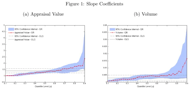
Figure 1 and Table 2 describe the private values quantile regression coefficients and 95%
confidence intervals for the estimates. The most interesting variable is the appraisal value,
a quality measure released by the seller, which is often interpreted as the seller’s private
value10. The associated quantile regression slope coefficient is given in the third column of
Table 2 and Figure 1a. Note that the coefficient is always significant and larger than 1,
suggesting that it acts as a markup indicating how much more the auctioned good appraisal
value is valued by the bidders than the seller. The private values can be also interpreted as a
measure of how much the bidders would be willing to sell goods made with the timber bought
at the auction11. This suggests that the higher the bidder’s private value, the higher is his
efficiency in aggregating value to the timber. The relative markup over the appraisal value
10
See Lu and Perrigne (2008) and Aradillas-Lopez et al. (2013)
11
In this interpretation, it is necessary to assume that timber is the most important component of the
goods produced by the bidders. This could be however modified to cover other cases where timber would
increases by about 75% when comparing bidders in the α= 0.10 and α = 0.80 quantiles of
the private value conditional distribution. This is also evidence that bidders belonging to
the upper tail of the private value distribution are more highly affected by changes in the
appraisal value than median bidders. A test to investigate constancy of the slope coefficient
has been applied showing significant change in the slope quantile regression coefficients across
A12. Figure 1a and 1b give, respectively, the quantile regression and OLS estimates of the
appraisal value and volume with their corresponding 95% confidence intervals.
Figure 1: Slope Coefficients
(a) Appraisal Value (b) Volume
The 95% confidence intervals for the OLS estimate consider the heteroscedasticity-robust (White) standard errors. The ones for the quantile regression estimates were computed by resampling with replacement the (Xℓ, Wℓ)-pair in each original
subsampleLn.
12
Table 2
Private Value Quantile Regression Estimates
Quantile Level Intercept Appraisal Value Volume
0.1 0.95 1.01 0.0007
[-0.97,2.28] [0.99,1.04] [0.0004,0.0016]
0.2 3.00 1.04 0.0016
[-0.72,8.49] [0.99,1.13] [0.0005,0.0027]
0.3 9.39 1.15 0.0018
[2.05,15.01] [1.05,1.22] [0.0010,0.0033]
0.4 11.77 1.25 0.0034
[5.32,20.83] [1.14,1.33] [0.0013,0.0049]
0.5 21.03 1.29 0.0041
[10.92,29.24] [1.22,1.43] [0.0023,0.0054]
0.6 35.68 1.36 0.0041
[21.63,45.02] [1.27,1.56] [0.0029,0.0055]
0.7 44.28 1.57 0.0045
[29.94,77.15] [1.22,1.81] [0.0029,0.0071]
0.8 67.64 1.75 0.0060
[32.91,101.02] [1.31,2.02] [0.0024,0.0138]
0.9 72.98 2.37 0.0167
[12.89,124.22] [1.54,4.56] [0.0031,0.0384]
The estimates are for a median auction. The 95% confidence interval in square brack-ets were computed by resampling with replacement the (Xℓ, Wℓ)-pair in each original
subsampleLn;
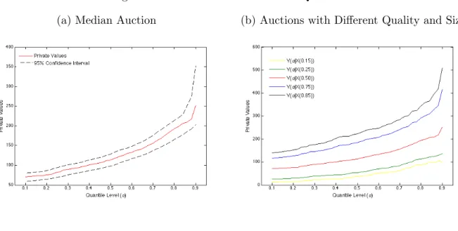
With some abuse of terminology,X(τ) = (X1(τ), X2(τ), X3(τ)), forX1(τ) a column vector
of ones, denotes the quantile of order τ of the matrix of auction covariates X, i.e. X(0.50)
represents median auctions. Figure 2a gives the private value conditional quantile estimates
for a median auction and their 95% confidence intervals. In a median auction, the volume
is 967 thousand of board feet and the appraisal value is about $68 per thousand of board
feet. Figure 2b presents the quantile estimates for several quantile levels of X(τ), where
τ ={0.15,0.25,0.50,0.75,0.85}. In particular, it shows how the shape of the private value
quantiles change due to variations in the quality and size of the timber tract. This effect
becomes clearer when comparing a high with a low quantile of the private value conditional
distribution. Consider in particular α = 0.12 and α= 0.80 for X(τ), τ ={0.15,0.50,0.85},
that is, auctions with low, median and high quality and size. The relative increase in the
private value is of about 600% in auctions with low quality and size, whereas it reduces to
172% and 142% in median and high quality and size auctions, respectively.
Figure 2: Private Values Conditional Quantiles
(a) Median Auction (b) Auctions with Different Quality and Size
We now turn to the estimation of the seller’s expected payoff and the associated optimal
to determine the optimal screening level policy since it represents the possible gains the
seller may have when selling the good in the outside market. Note that V0(X) = 0 may
represent the case in which the seller has no opportunity to sell the good outside the auction.
The most common choice for V0(X) is the appraisal value of the timber13. The results
obtained for V0(X) = Appraisal Value (AV) are compared with the case with no outside
option V0(X) = 0.
Table 3 gives the estimates of the optimal screening level αbR(X, V0), the corresponding
optimal reservation priceRb(X, V0) and the seller optimal expected payoffΠ (b αbR|X, N, V0(X))
for both choices ofV0(X) and auctions with different quality and size. The optimal screening
levelαbR(X, V0) is chosen as the maximizer of the seller’s expected payoff14 overA. A general
conclusion from Table 3 is that auctions with higher quality and size provide larger expected
payoffs for the seller, whereas the optimal screening level reduces. A possible reason for that
is the low heterogeneity among bidders observed in better auctions15. Therefore, as seen
from Proposition 2.9, the seller has a strong incentive to use screening for low quality and
size auctioned goods, whereas the seller private value’s choice does not seem to affect his
reservation price policy in these cases.
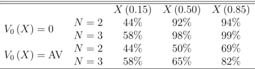
As mentioned in Section 2.1, the probability of trading in the auction with a screening
level αR(X) is 1−αR(X)N. Table 4 groups the probabilities of trading under an optimal
13
As mentioned in Aradillas-Lopez et al. (2013), the seller’s private value may be even lower than the
appraisal value of the timber if exercising an outside option (through, for example, a lump-sum contract)
entails additional cost to the seller. It is also possible thatV0(X) is nevertheless higher than the appraisal
value since scaled sales require the timber service to measure the timber actually harvested to calculate the
payment. Therefore, by exercising the outside option the seller would avoid those costs.
14
The definite integral in (2.9) is estimated via numerical integration using a trapezoidal rule overA.
15
Recall from Figure 2b that auctions with low quality and size show a significant increase in the markup
Table 3
Optimal Reservation Price
Seller’s Private Value
V0(X) = 0 V0(X) = AV
b
αR(X(0.15), V0) 0.75 0.75
[0.52,0.80] [0.56,0.80]
b
R(X(0.15), V0) 83.08 83.08
[38.93,104.58] [45.34,109.03]
b
Π (αbR|X(0.15),2, V0) 32.64 39.05
[26.16,44.78] [30.26,50.33]
b
Π (αbR|X(0.15),3, V0) 38.98 43.80
[30.62,52.92] [33.32,56.73]
b
αR(X(0.50), V0) 0.28 0.71
[0.12,0.36] [0.56,0.78]
b
R(X(0.50), V0) 87.93 159.89
[67.73,101.96] [123.40,192.43]
b
Π (αbR|X(0.50),2, V0) 91.71 108.49
[79.17,102.32] [95.11,122.13]
b
Π (αbR|X(0.50),3, V0) 102.93 112.50
[99,126.57] [89.63,114.26]
b
αR(X(0.85), V0) 0.24 0.56
[0.12,0.42] [0.47,0.80]
b
R(X(0.85), V0) 163.65 243.97
[135.51,213.63] [220.03,376.25]
b
Π (αbR|X(0.85),2, V0) 177.66 203.26
[163.40,192.73] [187.71,223.19]
b
Π (αbR|X(0.85),3, V0) 196.37 208.61
[179.89,212.72] [191.63,231.26]
The 95% confidence intervals in square brackets were computed by re-sampling with replacement the (Xℓ, Wℓ)-pair in each original subsample
Ln.
screening level policy according to (X(τ), V0(X)) and for τ ={0.15,0.50,0.85}. Note that
and 58% forN = 2 andN = 3, respectively). This is because bidders are very heterogeneous
and the seller should set a high screening level to avoid low bidders from participating. This
somehow carries over for median and higher quality and size auctions when the seller’s private
value is the appraisal value. Policy recommendations with such a low probability of selling
may not make sense in practice, especially for goods with a potential high storage cost. This
effect seems to be less expressive when the seller faces no outside option. As can be seen, the
practical implementation of the auction theory can be sometimes difficult in the sense that
usual choices for the seller’s private value may lead to recommendation of mechanisms with
very low probability of trading. This may question the relevance of considering expected
payoff in the maximization process.
Table 4: Probability of Trading
X(0.15) X(0.50) X(0.85)
V0(X) = 0 NN = 2= 3 44%58% 92%98% 94%99%
V0(X) = AV N = 2 44% 50% 69%
N = 3 58% 65% 82%
6
Conclusion
This paper proposes an identification and estimation approach based on quantile
regres-sion to recover the bidders’ private values conditional distribution. The quantile regresregres-sion
framework provides a flexible and convenient parametrization of the private value
distri-bution, with an estimation methodology easy to implement and with various specification
tests that can be derived. The paper shows that a focus on the quantile level of the private
values distribution, in particular the optimal screening level, can be very useful for policy
The empirical application using timber auctions from the USFS shows that policy
rec-ommendations should be carefully examined before practical implementation. The screening
level associated with the optimal reservation price is fairly high in general, resulting in a low
probability of trading. The analysis of the shape of the private value conditional quantile
curves suggests that such inappropriate recommendations are due to a sharp increase in the
private value conditional quantiles, which may be evidence of large heterogeneity among the
bidders. As a consequence, the seller has a strong incentive to screen bidders’ participation
by using a high reservation price, leading then to a low probability of selling the auctioned
good.
The estimated private values quantile shapes can be genuine but can also be the
con-sequence of a model misspecification. It would be for instance interesting to investigate
identification under a more flexible, and perhaps unknown, quantile specification function.
Gimenes and Guerre (2014) have suggested a sieve interactive quantile specification in the
setup of first-price sealed bid auctions, which can cope with dimension reduction issues while
still very flexible and with nonparametric features.
Regarding the consequences of the quantile shapes for policy recommendations, some
other works have also noticed such a high level of the optimal reservation price in timber
auctions. Aradillas-Lopez et al. (2013) suggest that neglecting private values affiliation can
generate high reservation prices. However, their nonparametric methodology may be affected
by the curse of dimensionality. In addition, as noted in Roberts and Sweeting (2013), timber
auctions include a preliminary selection that can affect the estimated shape of the private
value quantile functions. The large heterogeneity revealed by the estimation of the private
value conditional quantile function can also be an indication of asymmetry. As discussed
in Cantillon (2008) and Gavious and Minchunk (2012), sellers facing asymmetry have an
However, analysing revenue with a risk neutral seller perspective may not be appropriate
to address issues such as high reservation prices and low probability of selling the auctioned
object. The results given in Hu, Matthews and Zou (2010) regarding risk aversion affecting
sellers can be useful to provide more relevant reservation price recommendations. Gimenes
(2014) proposes a numerical investigation of the variation in the optimal screening level when
the seller has a constant relative risk aversion utility function and concludes that considering
risk averse sellers is indeed sufficient to achieve reasonable policy recommendations.
References
[1] Aradillas-Lopez, Andres, Amit Gandhi & Daniel Quint (2013). Identification
and inference in ascending auctions with correlated private values. Econometrica, 81,
489-534.
[2] Athey, Susan, Jonathan Levin (2001). Information and competition in U.S. forest
service timber auctions. Journal of Political Economy, 109, 375-417.
[3] Athey, Susan & Philip A. Haile (2002). Identification of standard auction models.
Econometrica, 70, 2107-2140.
[4] Baldwin, Laura H., Robert C. Marshall & Jean-Francois Richard (1997).
Bidder collusion at Forest Service Timber Sales. Journal of Political Economy, 105,
657-699.
[5] Bassett, G. (1988). A property of the observations fit by the extreme regression
[6] Bassett, Gilbert & Roger Koenker (1978). Regression quantiles. Econometrica,
46, 33-50.
[7] Bassett, G. & R. Koenker(1982). An empirical quantile function for linear models
with iid errors. The Journal of the American Statistical Association 77, 407-415.
[8] Bikhchandani, Sushil, Philip A. Haile & John G. Riley (2002). Symmetric
separating equilibria in English auctions. Games and Economic Behavior, 38, 19-27.
[9] Buchinsky, Moshe (1995). Estimating the asymptotic covariance matrix for quantile
regression models: a Monte Carlo study. Journal of Econometrics, 68, 303-338.
[10] Campo, Sandra, Emmanuel Guerre, Isabelle Perrigne & Quang Vuong
(2011). Semiparametric estimation of first-price auctions with risk averse bidders.Review
of Economic Studies, 78, 112-147.
[11] Cantillon, Estelle(2008). The effect of bidders’ asymmetries on expected revenue
in auctions. Games and Economic Behavior, 62, 1-25.
[12] Chernozhukov, V.(2005). Extremal quantile regression.The Annals of Statistics 33.
806-839.
[13] Donald, Stephen G. & Harry J. Paarsch (1993). Piecewise pseudo-maximum
likelihood estimation in empirical models of auctions. International Economic Review,
34, 121-148.
[14] Donald, Stephen G. & Harry J. Paarsch (1996). Identification, estimation, and
testing in parametric empirical models of auctions within the independent private values
[15] Gavious, Arieh & Yizhaq Minchuk (2012). A note on the effect of asymmetry on
revenue in second-price auctions. International Game Theory Review, 14, Issue 03.
[16] Gentry, Matthew & Tong Li(2014). Identification in auctions with selective entry.
Econometrica, 82, 315-344.
[17] Gimenes, Nathalie (2014). To Sell or not to Sell? An Empirical Analysis of the
Optimal Reservation Price in Ascending Timber Auctions. Working Paper. Department
of Economics, University of Sao Paulo.
[18] Gimenes, Nathalie & Emmanuel Guerre (2014). Parametric and nonparametric
quantile regression methods for first-price auction: a signal approach. Working Paper.
Queen Mary, University of London.
[19] Guerre, Emmanuel, Isabelle Perrigne & Quang Vuong (2000). Optimal
non-parametric estimation of first-price auctions. Econometrica, 68, 525-574.
[20] Guerre, Emmanuel & Camille Sabbah (2012). Uniform bias study and Bahadur
representation for local polynomial estimators of the conditional quantile function.
Econometric Theory, 28, 87-129.
[21] Haile, Philip A. (2001). Auctions with resale markets: an application to U.S. Forest
Service Timber Sales. American Economic Review, 91, 399-427.
[22] Haile, Philip A. & Elie Tamer (2003). Inference with an incomplete model of
English auctions. Journal of Political Economy, 111, 1-51.
[23] Haile, Philip A., Han Hong & Matthew Shum (2003). Nonparametric tests for
[24] Hu, Audrey, Steven A. Matthews & Liang Zou (2010). Risk aversion and
optimal reserve prices in first- and second-price auctions. Journal of Economic Theory,
145, 1188-1202.
[25] Koenker, Roger(2005). Quantile Regression. Cambridge Books, Cambridge
Univer-sity Press.
[26] Krishna, Vijay (2010). Auction Theory. Academic Press.
[27] Laffont, Jean-Jacques, Herve Ossard & Quang Vuong (1995). Econometrics
of first-price auctions. Econometrica 63, 953-980.
[28] Li, Tong & Isabelle Perrigne (2003). Timber sale auctions with random reserve
prices. Review of Economics and Statistics, 85, 189-200.
[29] Li, Tong, Isabelle Perrigne & Quang Vuong(2003). Semiparametric estimation
of the optimal reserve price in first-price auctions. Journal of Business and Economic
Statistics, 21, 53-64.
[30] Li, Tong & Xiaoyong Zheng (2009). Entry and competition effects in first-price
auctions: theory and evidence from procurement auctions.Review of Economic Studies,
76, 1397-1429.
[31] Li, Tong & Xiaoyong Zheng (2012). Information acquisition and/or bid
prepa-ration: a structural analysis of entry and bidding in timber sale auctions. Journal of
Econometrics,168, 29-46.
[32] Lu, Jingfeng & Isabelle Perrigne(2008). Estimating risk aversion from ascending
and sealed-bid auctions: the case of timber auction data.Journal of Applied
[33] Marmer, Vadim, & Artyom Shneyerov (2012). Quantile-based nonparametric
inference for first-price auctions. Journal of Econometrics, 167, 345-357.
[34] Marmer, Vadim, Artyom Shneyerov & Pai Xu (2013). What model for entry in
first-price auctions? A nonparametric approach. Journal of Econometrics, 176, 46-58.
[35] Menzel, Konrad, & Paolo Morganti (2013). Large sample properties for
esti-mators based on the order statistics approach in auctions. Quantitative Economics, 4,
329-375.
[36] Myerson, Roger B.(1981). Optimal auction design. Mathematics of Operations
Re-search, 6, 58-63.
[37] Newey, Whitney & Daniel McFadden (1994). Large sample estimation and
hy-pothesis testing. In Handbook of Econometrics, 4, Ch. 36. Elsevier Science.
[38] Paarsch, Harry J. (1992). Deciding between the common and private value
paradigms in empirical models of auctions. Journal of Econometrics, 51, 191-215.
[39] Powell, James L. (1991). Estimation of monotonic regression models under quantile
restrictions, in Nonparametric and Semiparametric Methods in Econometrics, (ed. by
William A. Barnett, James L. Powell and George E. Tauchen), Cambridge: Cambridge
University Press.
[40] Rao, C. Radhakrishna, & L.C. Zhao (1992). Approximation to the distribution of
M-estimates in linear models by randomly weighted bootstrap. Sankhya 54, 323-331.
[41] Rezende, Leonardo (2008). Econometrics of auctions by least squares. Journal of
[42] Riley, John G., & William F. Samuelson (1981). Optimal auctions. American
Economic Review 71, 381-392.
[43] Roberts, J. & A. Sweeting (2013). When Should Sellers Use Auctions? American
Economic Review 103, 1830-1861.
[44] Wang, Xiao M. & Wang Zhou (2004). Bootstrap approximation to the distribution
of M-estimates in a linear model. Acta Mathematica Sinica, 20, 93-104.
[45] Zhao, Lin-cheng, Xiao-yan Wu & Ya-ning Yang (2007). Approximation by
ran-dom weighting method for M-test in linear models. Science in China Series A: