.-
._-....
セfundaᅦᅢo@
....
GETULIO VARGAS
EPGE
SEMINÁRIOS
DE PES"QUISA
ECONOMICA
Escolade
Pós-Graduação emEconomia
"An
Emplrlcal ComparlaoD
of
Forward-Rate and Spot-Rate
Modela
for
Valulnglnterest-Rate
Optlona"
Prof. Wolfgang Bühler
(University ofMannheim-Germany)
LOCAL
Fundação Getulio Vargas
Praia de Botafogo, 190 - 10" andar - Auditório
DATA
12/08//99
(58
feira)
HORÁRIO
16:00h
Coordenação:
Proc.
Pedro Cavalcanti Gomes Ferreirar
.,
TI/E JOURNAL OF FINANCE • VOL. LlV, NO. 1 • FEBRUARY 1999
An
Empirical Comparison of Forward-Rate
and Spot-Rate Models for Valuing
Interest-Rate Options
WOLFGANG BÜHLER, MARLIESE UHRIG-HOMBURG, ULRICH WALTER, and THOMAS WEBER*
ABSTRACT
Our main goal is to investigate the question of which interest-rate options valua-tion models are better suited to support the management of interest-rate risk. We use the German market to test seven spot-rate and forward-rate models with one and two factors for interest-rate warrants for the period from 1990 to 1993. We identify a one-factor forward-rate model and two spot-rate models with two faetors that are not significant1y outperformed by any of the other four models. Further rankings are possible if additional cri teria are applied.
A VALUATION MODEL FOR INTEREST-RATE derivatives represents the core ofany
sys-tem designed to measure, control, and supervise interest-rate risk. This is true regardless ofwhether a value-at-risk methodology, sensitivity analysis, stress test, or scenario technique is applied. Unfortunately, there is no empirical ev-idence that evaluates the performance ofthe most popular competing pricing models using the some data from a risk management perspective. This paper provides such empirical evidence using data from the German market for interest-rate warrants for the period from 1990 to 1993,
The more recent valuation models are dominated by two groups of models, forward-rate and spot-rate models, The approach of the first group, pio-neered by Ho and Lee (1986) and Heath, Jarrow, and Morton (HJM) (1992), directly uses the arbitrage-free dynamics of the entire zero bond price curve or, equivalently, the term structure of forward rates to price interest-rate derivatives. We refer to this approach as the forward-rate (or HJM) model. The approach of the second group (e.g., see HulI and White (1990, 1993), B1ack, Derman, and Toy (1990), B1ack and Karasinski (1991), Jamshidian (1991), and Sandmann and Sondermann (1993» is based on the dynamics of
• Bühler and Uhrig-Homburg are from the University of Mannheim, Germany. Walter is at Deutsche Genossenschaftsbank, Germany. Weber is at Infinity FinanciaI Technology, London. We thank Michael Dempster, Darrell Dume, Stewart Hodges, Wolfgang Schmidt, and Dieter Sondermann. We are especially grateful for the comments by Stephen Figlewski, OIaf Kom, and Stuart 'fumbull. The paper has also great1y benefited from comments made at the War-wick Option Conference 1995, the European FinanciaI Management Association Conference 1997, and the Finance seminars at Ecole Supérieure des Sciences Economiques et Commer-ciales, Paris; Eidgen6ssische Hochschule, ZUrich; and Erasmus University, Rotterdam. Addi-tional thanks go to an anonymous referee and René Stulz for helping us to sharpen our focus.
270 The Journal of Finance
the instantaneous spot interest rate. The second group's papers follow a suggestion by Cox, Ingersoll, and Ross (1985) and fit the endogenous term structure (and volatility structure) of interest rates to the observed term structure. This fitting is achieved through time-dependent parameters of the stochastic factor processes. Both approaches that model the stochastic be-havior of the term structure of interest rates, as well as the subsequent valuation of derivatives, are closely related to each other. In fact, for some of the models, a mathematical equivalence is easily established.
In this comprehensive empirical study we test one-factor and two-factor spot-rate and forward-spot-rate models. The paper's main goal is to clarify the question ofwhether spot- or forward-rate models are better suited to support the mea-surement, control, and supervision of interest-rate risk. Existing work pro-vides no answer to this important questiono Though the two classes ofmodels are close to each other from a theoretical point of view, they can exhibit very different behaviors in application. Furthermore, it is not at alI obvious whether two-factor models outperform one-factor models in each class.
The models we test have the folIowing basic structures. The one-factor spot-rate model is characterized by a mean-reverting drift and a diffusion coefficient with constant elasticity. Within the class of two-factor spot-rate models we consider two variants: In the first model, the factors are identi-fied with a long rate and the difference between this long rate and a short rate. In the second model, the factors we consider are the short rate and its volatility. These two-factor models represent generalizations of models de-veloped by Schaefer and Schwartz (1984) and Longstaff and Schwartz (1992).
We test two forward-rate models with one factor. The first model repre-sents the continuous-time version ofHo and Lee's (1986) model with Gauss-ian forward rates and constant (absolute) volatility. The second model has a linear proportional volatility-that is, the proportional volatility depends solely on time-to-maturity of forward rates. We ais o test two forward-rate models with two factors. We determine the volatility functions of both mod-eIs by principal component analyses. The volatilities, therefore, depend on empiricalIy specified factor loadings and these factors' volatilities. In one model, forward-rate volatilities are independent offorward rates. In the other, they are proportionally dependent on these rates.
Assessing the applicability of the different mo deis within a risk manage-ment system requires two important decisions about the test methodology. First, valuation models within risk management systems must be capable of predicting future option prices if they are to correctIy measure risk expo-sure. This capability is best evaluated by the ex ante predictability of a model. Therefore, we use the valuation quality of a model, not its ability to identify mispriced options, as the most important assessment criterion. This implies that this study is not a test of an option market's efficiency.
Second, we estimate alI parameters, including the volatility, from time series. There are two reasons to estimate parameters historically rather than implicitIy. We cannot prematurely rule out that model-dependent param-eters, such as implied volatilities, favor one model versus the other. More important, testing valuation models with implied parameters only
repre-!.
•
"
.
Comparison of Models for Valuing /nterest-Rate Options 271
sents a "local test," in the sense that the current option price is used to value the same option one period later. Therefore, "local tests" consider only smalI deviations from observed prices of derivatives. Tests on the basis of histor-icalIy estimated parameters are "global," in the sense that they do not use information from derivatives markets.
In addition to the valuation quality, there are other important cri teria for assessing a valuation model for interest-rate options. These refer to the dif-ficulties in estimating the mo dei parameters, in fitting the model to the cur-rent term and volatility structures, in computing the option values numericalIy, and to the stability of the moders performance over different time periods.
We test the seven valuation models for interest-rate warrants from the German market for the period from 1990 to 1993. In contrast to standard-ized options traded on the German Futures and Options Exchange (DTB) in Frankfurt, interest-rate warrants are options issued by banks. Underlying these warrants are German government bonds, which represent the most Iiquid market segment in the German bond market. The market for interest-rate warrants started in 1989 and is now more Iiquid than the market of standardized options on the BUND-Future that are traded on the DTB. We ais o selected this market segment of German interest-rate options beca use warrants show a much wider variety of terms than do standardized options. There are warrants of both the European and American types whose matu-rities range up to 2.9 years, compared with nine months' for the standard-ized futures options on the BUND-Future.
Very few papers study the empirical performance of models for the valua-tion of interest-rate opvalua-tions. Dietrich-Campbell and Schwartz (1986) value interest-rate options on U.S. government bonds and treasury bills, using the two-factor Brennan and Schwartz (1982) mode!. Bühler and Schulze (1995), Flesaker (1993), andAmin and Morton (1994) present empirical studies ofthe HJM model. The study by Bühler and Schulze analyzes the optimal call policy of callable bonds that are issued by German public authorities. Flesaker, as well as Amin and Morton, presents results for Eurodollar futures options. How-ever, none of these studies compares spot-rate and forward-rate models.
The paper is organized as follows. In Section I we describe our selection of the empiricalIy tested models on the basis of an extensive data analysis and the decisions made in the different implementation steps. Section II presents relevant information on the German bond and interest-rate options market. In Section III we describe the design of the empirical study and provide estimation results for the input data of the different models. The valuation results, including a multivariate error analysis and a paired comparison of the seven models, appear in Section IV. We summarize our final assessment qf the models and present conclusions in Section V.
I. Selected Valuation Models and Their Implementation In this section, we describe our selection of the empirically tested spot-rate and forward-spot-rate models. We also specify the formal structure of the models and describe the decisions made in the different implementation steps.
I
ii
272 The Journal of Finance
A. Data Analysis and Selection of Models
The first step in testing interest-rate options valuation models is to pre-select the basic features of the models. Prepre-selection refers to the number of faetors driving the term structure of interest rates and the functional form of the stochastic processes for these faetors. Th do this, we perform an ex-tensive data analysis of the faetor structure of zero bond yields and the behavior of individual yields in the German bond market. We then summa-rize our findings, which are the basis of the models discussed in Section LB. The details are presented in Bühler et aI. (1996).
We first apply principal component analyses to determine the number of factors. Because of the high degree of correlation among yields with differ-ent maturities, two faetors explain more than 95 percdiffer-ent of the variation in the term structure of interest rates. These findings are stable over different
time periods with varying lengths during 1970 to 1993. Litterman and
Scheink-man (1991) report similar results for the U.S. market. On the basis of these results, we only consider one- and two-factor models. One-faetor models should be understood as a reference case against which we measure the improve-ment of introducing a second faetor. Of course, to understand whether two faetors are sufficient, the whole study should be carried out for three faetors.
A.l. One-Factor Models
The distinguishing feature of a one-faetor forward-rate model is the func-tional form of the forward-rate volatility. Amin and Morton (1994) test dif-ferent parsimonious (one and two para meter) parameterizations and find that the number of parameters has a stronger effect on the behavior of the model than does the form ofthe models used. 'I\vo-parameter models tend to
fit prices better. Indeed, the model with the best fit in-sample and
out-of-sample is the two-parameter model with a linear proportional volatility func-tion. However, the one-parameter models result in implied para meter estimates that are more stable, and the models earn larger and more consistent profits from their perceived mispricings. Amin and Morton conclude that the model with constant volatility (the absolute model) seems to be preferable among the ッョ・セー。イ。ュ・エ・イ@ models.1
In light of these findings, we test two factor HJM models, a one-parameter and a two-one-parameter model. The one-one-parameter model we choose for our investigation is the one with constant volatility, which is in fact the continuous-time version of the Ho and Lee model. The two-parameter model is the one with linear proportional volatility.
One-faetor spot-rate models start with a specification of the process of the
short rate, r. In line with studies for other markets, we find that an increase
(decrease) in short rates is more likely than a decrease (increase) if the values of the rates are historically low (high). Additionally, large interest-rate movements take place in periods of high interest interest-rates, and modeinterest-rate
1 Arnin and Morton (1994) test the HJM models using Eurodollar futures and options. Some
of their resulta might stem from the short maturity of the options considered.
セ@
._----
--- --------
..-"
Comparison of Models for Valuing Interest·Rate Options 273
movements are observed in low-rate periods.2 Therefore, we use the standard
model for the short rate, a mean-reverting process with an instantaneous
vol-atility shown as ur'. Contrary to the results ofChan et aI. (1992), who report
a value of 1.5 for the exponent E, we find values between 0.5 and 1.3 These
es-timates result in a unique solution of the stochastic differential equation of r.
A.2. 1loo·Factor Models
For a two-faetor forward-rate model, two volatility functions-one for each factor-must be specified. We consider two different structural specifica-tions. In the first case, we assume that both volatility functions are inde-pendent of the forward rate's leveI. In the second case, the two volatility functions are proportional to the forward rates. We empirically determine the precise functional form ofthe volatility funetions in both two-factor mod-eIs from principal component analyses.
Our choice of the state variables for the two two-faetor spot-rate models we investigate is motivated by two empirical findings. First, principal com-ponent analyses in combination with regression analyses reveal that the first component can be identified with the leveI of the yield curvei the
sec-ond is closely related to the spread between the long and the short rate.4 We
take these findings as a guideline for the construction of our first two-factor model, which uses both a long rate and the spread between the aRme long rate and the short rate as faetors. The basic idea for this line of approach goes back to Brennan and Schwartz (1979) and Schaefer and Schwartz (1984). The second two-factor model is based on the observation that the short-rate volatility exhibits typical volatility clusterings. Therefore, a model with stochastic volatility of the short rate could be an appropriate description of the data. This model representa a generalization ofthe Longstaffand Schwartz
(1992) approach.
Both two-faetor spot-rate models are special cases ofthe affine class ofterm strueture models. (See Duffie and Kan (1996), pp. 383-391.) Although they are mathematically equivalent, empirically, they can behave very differently.
B. Review of the Models and Basic Implementation Steps
B.l. The Forward-Rate Models
Here, we briefly review the HJM approach and the concrete implementa-tion realized in this study. Rather than discussing the approach in general terms, we concentra te on the simplest derivation for the forward-rate mod-eIs that we use in our empirical investigation.
2 See Chan et a!. (1992) for the U.S. market, Barone at a!. (1991) for the Italian market, and
Walter (1996) for the German market ..
3 See Uhrig and Walter (1996). The details of this estimation procedure are discussed later.
I!, ., !;
274 1'he JOllrnal of Finance
Table I
Forward-Rate Models under Consideration
This table summarizes the parametric specification ofthe volatility functions. ,,(I,T,f) denotes
the volatiJity function for the one-factor models. ",(I,T,f) and ".(I,T,f) represent the two
vol-atiJity functions for the two-faclor models. f denotes the instantaneous forward rate at date I for
instantaneous borrowing or lending at date T (T '" I). (T, "o, and
u,
are positive parameters.",(I,T) and ".(I,T) are functions of I and T, which are to be empirically determined. In order
to avoid an explosion of the forward-rate processes in finite time, the proportional volatiJity is
capped by a large positive number M.
Panel A. One-Factor Models
u(I,T,f)
=
'T,T(I,T,f) ; (uo + 'T,(T - l))min(f,M)
",(I,T,f) = ",(I,T) ".(I,T,f) ; ".(I,T)
Panel B. 'l\yo-Faclor Models
",(I,T,f) = ",(I,T)min«(,M)
".(I,T,f) ; u.(I,T)min(f,M)
Absolute I Linear proportional
Absolute 11
Proportional 11
The fundamental building block of this approach is the whole instanta-neous forward-rate curve. HJM start with a fixed number of unspecified
factors that drive the dynamics of these forward rates:5
2
df(t,T) = a(t,T,·) dt +
L
ui(t,T,f)dzi(t), (1);=1
where f(t, T) denotes the instantaneous forward interest rate at date t for
borrowirig or lending at date T (T;;:: t), Zl(t) and Z2(t) denote independent
one-dimensional Brownian motions, and a(t,T,') and ui(t,T,f) are the drift
and the volatility coefficients of the forward rate of maturity T. As HJM
show, when a number' of regularity conditions and a standard no-arbitrage condition are satisfied, then the drift of the forward rates under the
risk-neutral measure is uniquely determined by the volatility functions ui(t, T, f):
2
fT
a(t,T,') = ゥセ@ Ui(t,T,f) I ui(t,s,f)ds. (2)
As we noted earlier, we focus on four specifications of this approach: two one-factor mo deIs and two two-factor models. The parametric specification
of the volatility functions is shown in Table I.
• In the following, we concentrate on two factors. In general, drift and volatilities can depend on the path of the forward-rate curve. See Heath et aI. (1992), p. 80.
Comparison of Models for Vallling lnterest-Rate Options 275
The first step in implementing any particular valuation model for interest-rate derivatives is to estimate the current yield curve, which is used in the
forward-rate models in the form of the current forward-rate curve f(O,T).
We discuss the term structure estimation procedure in detail in Section IH. In the second step, we estimate the volatility parameters. As discussed ear-lier, we estimate these parameters from time-series observations of forward rates. We obtain the volatility parameters of the two one-factor models di-rectly from forward-rate changes and relative forward-rate changes, respectively.
By means of principal component analyses, we determine the volatilities
of the forward rates f(t,T) in the two-factor models by the faetor loadings
and the volatilities of the two independent faetors.
In the third step, we compute the option prices. In this step, we discretize equation (1) under the risk-neutral measure by building a binomial tree model. This tree is nonrecombining for the Linear Proportional and the Proportional H forward-rate models. Supporting the findings of Amin and Morton (1994), we find that seven time steps are sufficient to achieve accurate option prices. A seven-step binomial nonrecombining tree contains 254 (128 final) nodes for the one-faetor models and 3,279 (2,187 final) nodes for the two-faetor models. As usual, in the backward induction procedure we consider the premature ex-ercise feature of American options, taking at each node the maximum of the intrinsic value and the value of the option if not exercised.
B.2. The Spot-Rate Models
Unlike the forward-rate models that define the stochastic behavior of the term strueture relative to the observable current term structure, spot-rate models must be adapted to the current interest rates and volatilities. Fol-lowing a suggestion made by Cox et aI. (1985), we achieve this adaptation through time-dependent parameters of the stochastic faetor processes. These time-dependent parameters are determined in such a way that both the en-dogenous term and volatility struetures fit with the observable one. In prin-cipIe, this requires an inversion of the valuation formula.
In our approach, we base the inversion of the spot-rate models on the fundamental valuation equation for derivatives as derived in the general equilibrium setting by Cox et aI. (1985).6 If the value of a derivative with
payofT at time Tis a sufficiently smooth funetion F(Xlox2' t,T) of time and
two independent difTusion processes Xl' X2 with drift and difTusion functions
lLi(Xi,t), Ui(Xi,t), i = 1,2, then F satisfies the following partial difTerential
equation in the no-exerci se region:
F, + Fx,[ILI - 0l
ud
+ Fx.[1L2 - 02U2] + Fx,xJuf + fxRxRセオゥ@ = rF, (3)6 See Cox et aI. (1985), p. 388. For an exposition of the Hull and White approach, refer to
Hull and White (1990). A discrete variant is described in Hull and White (1993). For a presen-tation ofthe inversion problem in the framework of equivalent martingales, see Schmidt (1994),
p. 15.
,
276 The "Journal of Financewhere r represents the instantaneous risk-free rate, and 01(xI>x2,t) and
O2 (Xl,X2' t) are the market prices of risk for the two factors, It foIlows
from no-arbitrage arguments that 01 and O2 are real-valued functions of
only the state variables and time. The subscripts of F denote partial
de-rivatives. We obtain the values for contingent claims by solving this para-bolic partial differential equation subject to appropriate initial and boundary conditions.
In this study, we derive the three spot-rate models tested from equa-tion (3) by specifying the nature of the stochastic processes driving the fac-tors, the functional form ofthe market prices ofrisk, and the relation between the factors and the instantaneous spot rate, r. Table 11 summarizes the as-sumptions underlying the one-factor model and the models with two factors.
8.2.1. One-Factor Spot-Rate Model. The first model is a one-factor interest-rate model, in which we assume that the dynamics ofthe short-term interest
rate r(t) exhibit mean-reversion and that the diffusion coefficient depends
on the leveI of the short rate. K, 'Y, u, and € are positive constants.
The basic idea behind HuIl and White's (1990) procedure is to allow for
time-dependent parameters in the risk-neutralized process of r, in order to match the solution of equation (3), in the case of zero bonds, to an
exog-enously given term structure of zero bond prices. If the elasticity para meter
€ is positive, this calibration must be carried out numerically. Generally, any
of the parameters can be selected as a time-dependent function. However, for several economic and technical reasons, we select the market price of
risk as a time-dependent function.7 In principIe, if a second parameter is
assumed to depend on time, the model can aIs o be fitted to an exogenously given current volatility structure. However, this procedure has an important drawback: this second time-dependent parameter results in unstable and partially unrealistic future endogenous volatility structures. (HuIl and White
(1993, 1996) report similar results.)
In light of these findings, we do not calibrate the model to the whole cur-rent volatility structure with a second time-dependent para meter. Instead, we fit only two points of the endogenous volatility structure to the observ-able one, the volatilities of the short and the long rates. Volatilities of in-termediate rates are interpolated by the model.
The advantage of this parsimonious fitting procedure is that the model results in stable future volatility structures. Technically, we achieve the two-point calibration of the model to the current volatility structure by the
(con-stant) mean-reversion parameter K, which determines the transmission of
the instantaneous interest rate's volatility to the volatilities of long rates (cf.
Uhrig and Walter (1996), pp. 87-88).
7 The argumenta refer to the economic interpretation ofthe calibration process, the exiatence of a aolution for the fitting function, the conaequences for the endogenous volatility atructure, and the relation between riak-adjusted and original measure, Cf. "eath et aI. (1992), pp.96-97, and Uhrig and Walter (1996), pp. 84-85.
...
Comparison of Models for Valuing lnterest-Rate Options 277
セヲh@
セ@
il
.-4! セ@ ';; iuセ@ A I セ@
'sei!8.b セ@ セ@ 11
・ゥセウャNZ@
セ@
ô
....
' I : ' 3
ーNッG。IHNセ@ cu
QQAセQA@
セ@ Xセ@
';f:j's oS a' " , . ! o i セ@
NNAャセX@
Jl
セ@ セ@`セgI」オ@ . - t : ; -
-ッNNッセMァGウッs@ .. セセZZHッZZH@
""A a セM\@
OI "'.!i li) ,!!I 11 11 11 11 11
aセBGセセセ@
r::
\dセヲDセHjI@
,0 -g ã,:l
J:=
セGゥ@ ゥGセ@
セBLNァェセッセ@
NRセ。「セSQZャ@
M[ヲセA@ ... NLセ@
J.o セ@ ° セ@ A
GloS.:!Jlf & セ@ ..
ZRGZセ「oセセGB@ セセ@
セ@
,li
°GセNZA@
g
1:
gjセ@
..セ@ セ@
ッセセセBGM}@
:li.セ@
bbo .,
セ@ Jl oS .. t; b" + +J.of:..:2!;; .,
セ@
+Kセセ@
=GI"'i,S",,33 セ@ ⦅セセ@
Bcセ@ セ@ .... oo.... セ@ ",.,
gIセ@ fa",AA aí::' セii@
:a
"'..
'I: セ@セ@ f: I4'
セ@" ...
セ@
fIl]
8.セ@
..セ[[@
B /"- "';: •セセ@
'il .8 NLLセ@ セ@ "':< セ@ セ@ VGセ@ >1." >1. ...
GXセャAャ・NZAセセ@ 11 1111 1111
セ@
'"セAxャ@
'sセ@
,S {;セ@
{j-ll
セ@
'" OI" tl
セ@ {ャセGセ@
セセ@
&!,ua
2 1>./"-:-.ャセ ̄セヲセ@
セ@ "', .... 3'
o
セQセBGAャ@Q.""'A ュセ@
fi.) .. セ@
セ@
ゥZャセ@° '" [ '" セ@ '" 3.... f '" 3 "'.... oセ}ッャゥo@
!l
f:j.:! cu ou
セセャセ@
cuセ@ ゥセ@
:.=Ê
セ@ ,9 f$ セ@m
セ@ Lセセ@U) s= Q)"t;1'" セ@ =-=õ
LセDセセLXN@ セNN[^@
}Nゥセセセセ@
Q) セQエZャqIZZャ@セ@
セ^ゥLセ@
bQfraセXセ\i^セQ@
r::
Xセセ@BLセB@ [ - oS 3
.8 'til .. セ@ f: A "" oS
Gセ@
1! ] '"
A oS $1l ..
3°'" !I::t:
'" Jl セ@ °
'S
ti ".81
°'" .. セ@ '" "d - . < l
セB、BLB、セセ@ セセNLNLZ@
!l
ã
8
,!!IセN@
i:
セ@ セ@ セ@ セ@
セセZァ@
....
",b_ ] a{セs@'I: a
'ê
a b" rnoS
rn,
11-· セ@
\
278 The Journal of Finance
The model's implementation requires four steps. First, we determine the current yield curve of zero bonds from prices of coupon bonds. Second, we use an Euler-discretization to estima te the drift and volatility parameters of the short-rate processo We obtain the maximum Iikelihood estimates from time-series observations of the one-month money market rate. Third, we achieve the fitting to the current yield curve and to the volatility of the long
rate with maturity
T
= 9 years by using a numerical algorithm thatsimul-taneously determines the time-dependent function A(t) and the parameter K.
This requires the solution of the partial differential equation (3) with one
state variable XI = r under the foUowing conditions:
i. maturity condition for zero bonds: F(r,T,T) '" 1
iL fitting condition for endogenous zero bond prices to observed prices
i'(T) conditional on the current instantaneous rate, r(O):
F(r(O),O,T)
=
i'(T) (O<TsT) (4)iii. fitting condition for the volatility of the long rate:
1 Fr(r(O),O,T) A
- - = V.
T F(r(O),O, T) (5)
The left-hand side of equation (5) represents the ratio ofthe endogenous yield
volatility of a zero bond with maturity
T
and the short-rate volatility ur(O)<.The right-hand side denotes the ratio ofthe historical observed volatility ofthe
zero bond yield with maturity
T
and the short-rate volatility. We use thein-verted implicit finite difference method introduced by Uhrig and Walter (1996)
to solve equations (3)-(5).8 In the fourth and final step, we determine the
val-ues ofthe interest-rate warrants by solving equation (3) together with the ap-propriate boundary conditions for caUs and puts by a fully implicit
Crank-Nicholson method. We use a time step
t:.t
of one day for the time variable anda grid size of 1/30 for the transformed state variable z = 1/(1
+
r/r(O». Thischange.ofthe state variable, proposed by Brennan and Schwartz (1979), has
the advantage that the original state space [0,00) is transformed into the bounded
interval [0,1], and that the boundary conditions are easier to handle. For z = O
(r = 00) we use the fact that the values ofbonds and European options are zero,
and for z = 1 (r
=
O) we exploit numericaUy the special structure of thetrans-formed partial differential equation (3). We take into account the early exer-cise possibilities for American options in the recursive backward procedure.
B.2.2. 1Wo-Factor Model with Long Rate and Spread. The choice of the state variables in the second model is motivated by the findings in our data analysis process, and by the fact that the correlation among the changes of
8 Hull and White (1993) solve equations (3)-(5) on the basis of a trinomial tree, This method
can be considered as an explicit scheme. Cf. Brennan and Schwartz (1978), p. 464.
I
L
",
Comparison of Models for Valuing Interest-Rate Options 279
these two faetors is less than 0.23. These empirical observations suggest
that a two-factor model that uses a long-term rate l and the spread s
be-tween the long-term rate I and the short-term rate r as independent
sto-chastic factors can plausibly describe the yield curve dynamics.
An examination of the time-series behavior of long rates in the German
bond market reveals that there is only a slight mean-reversion tendency in long rates. The maximum Iikelihood estimate of the discrete version of the
process di = K/(n - l)dt
+
u/I<'dzl for the mean-reversion parameter K/ isnot significantIy different from zero on the 1 percent levei. As a proxy for the long rate, we use the yield to maturity of a nine-year zero bond.
To exdude, additionally, negative long rates I and to keep the model
ana-lyticaUy tractable, we mo dei the long rate as a martingale with a square root
representation
ul.Jl
of the diffusion coetricient.9 The spread process isas-sumed to foUow an Ornstein-Uhlenbeck process, in line with the observation that this process can take on both positive and negative values. The
param-eters UI, 1'., and u. are positive and constant.
We calibra te the model to the current term structure of interest rates by means of a time-dependent market price of spread risk. Because of the sep-arability of variables and the choice of an Ornstein-Uhlenbeck process for the spread, we can solve this problem analyticaUy. Moreover, this spread process ensures that the endogenous term structure of interest rates can be adapted to every observed one. This is not generaUy true for two-faetor mod-eis, which use nonnegative state variables.
We use the market price of long-term interest-rate risk to overcome a problem that is typical for two-faetor models in which both faetors are
in-terest rates (see also Dutrie and Kan (1996), p. 383). The state variable I is
labeled "Iong rate," but it does not have this property, since the price of a
zero bond depends on both state variables s and I. Therefore, a zero bond
with a maturity corresponding to I has a yield to maturity that does not rely
only on I. This internai inconsistency can be considerably reduced by an
appropriate choice of the market price of risk 81 of the long rate.1O
Again, the implementation of the model consists of four steps. The first step coincides with the first step of the one-factor mode!. The second step is reduced to an estimation of the two volatilities of the long rate and the spread. These two parameters also reflect the information about the vola-tility strueture. In the third step, the endogenous zero bond prices are an-alytically fitted to the observed prices by exploiting the separability of the
solution F(l,s, t,T) = G(l, t,T)H(s, t, T). FinalIy, we compute the option
val-ues by means of the alternating direction implicit method.11
9 However, this modeling has the drawback that for this process, I = O is an absorbing
barrier.
109
1 is chosen such that -(1/T)ln(F(I,8,t,t + T) = I holds for the specific time-to-maturity
of T = 10 years.
11 In contrast to the valuation of zero coupon bonds within the two-factor models, the
valu-ation of options on coupon bonds makes it necessary to solve a partial difTerential equvalu-ation in two state variables, beca use the terminal condition cannot be separated.
280 The Journal of Finance
The grid sizes for the time and state variables are fixed identically to that of the one-factor mode!. Because the state variable s can take on both pos-itive and nega tive values, we choose a special treatment. In the numerical
procedure, we restrict this state variable on the interval (-00,1 (O)]. We choose
the upper boundary 1(0) to ensure nonnegative short rates for the current
leveI of I. By an appropriate change of the state variable, we transform the
originalstate space (- 00,/(0)] into the state space [0,1]. For s
=
-00, we usethe fact that the values of bonds and European options are zero. For s
=
[(O)we impose a boundary condition, setting the second derivative F •• equal to
zero.
B.2.3. 1lvo-Factor Model with the Short Rate and Its Volatility. From our data analysis step, we know that the short rates exhibit volatility c1usters. This behavior can be modeled approximately by stochastic volatility. Since interest-rate volatility is a key variable in option pricing, a promising ap-proach might be to add to the one-factor model the leveI of interest-rate volatility as a second state variable.
The resulting model represents a generalized version of the general equi-Iibrium model proposed by Longstaff and Schwartz (1992). Longstaff and Schwartz base their model on assumptions about the stochastic evolution
of two abstract independent factors x and y, described in Table li, in which
Kx, Yx' u x' Ky, yy' and uy are (positive) parameters. The short-term rate r
and its instantaneous variance Vare determined endogenously as part of the equilibrium:
r=x+y
V=u;x+u;y.
(6)
(7)
Using this system of linear equations, we can represent the fundamental valuation equation (3) for interest-rate derivatives in terms of the
observ-able state variobserv-ables r and V.
1b achieve consistency with the current term structure, we generalize the model by allowing for a time-dependent risk parameter. Because of the
sep-arability of the partial differential equation in the state variables x and y,
we can reduce the adaptation ofthe endogenous to the exogenous term struc-ture of interest rates to the adaptation problem within the one-factor Cox et aI. (1985) model.
Again, the implementation procedure requires four steps. As in the other models, the first step involves the estimation of the current term structure of interest rates. Compared with the other two spot-rate models, the esti-mation of the parameters in the second step is more complex, beca use the volatility of the short-term rate is not directly observable. Following Long-staff and Schwartz (1993), we use a two-phase approach. In the first phase, we estimate the volatility of the short-term rate by using a generalized auto-regressive conditional heteroskedastic (GARCH) model. In the second phase,
Comparison of Models for Valuing Interest-Rate Options 281
we estima te the parameters describing the movement of the short-term in-terest rate and its volatility. 1b estimate these parameters, we equate the
first two moments of the long-run stationary unconditional distribution of r
and V with their historical counterparts.
In addition to these four equations, we obtain two further conditions by
choosing the volatility parameters
u;
andu;
as the minimum and themax-imum of the ratio V(t)/r(t), respectively. By using these six conditions, we
calculate the six parameters of the model by solving a nonlinear system of six equations.
The calibration of the model to the current term structure in the third step
follows the same procedure as the one-factor mode!. Again, we apply セィ・@
inverted implicit difference method. The computation of the option prices in the fourth step is comparable to the procedure in the other two-factor spot-rate model.
11. The German Fixed·Income Market
The German bond market is the third largest in the world. At year-end 1995, the nominal value of outstanding publicly issued bonds totaled more than three trillion deutsch marks (DM).
Traditionally, the bank bond sector is the largest component. However, bonds issued by the federal government are the most Iiquid. Typically,
so-called Bundesanleihen (BUNDs) are issued with an initial maturity of ten
years and Bundesobligationen (BOBLs) with an initial maturity offive years.
BUNDs are termed as long term, and BOBLs as medium termo Various interest-rate derivatives have been launched in the last seven years, ofwhich the BUND-Future (futures on ten-year government bonds) at the Deutsche TerminbOrse is the most popular.
Three types ofinterest-rate options trade in Germany: options on the BUND-Future and on the BOBL-BUND-Future (futures on five-year government bonds), interest-rate warrants, and over-the-counter (OTC) interest-rate options of ali types.
Because the market for options on futures is not particularly Iiquid and sufficient1y long-term time-series data are not available for OTC-options, our empirical study is based on the valuation of interest-rate warrants. Un-derlying these warrants are German government bonds. Most of them are the American type, with maturities of up to three years. Therefore, they represent a more diverse sample than would standardized options traded at options exchanges.
A. Government Bonds
" i
.,
セ@'.
282 The Journal of Filla/lce
considered in our study. In the period from 1990 to 1993, the coupons of these bonds varied between 5 percent and 10.75 percent. The initial matu-rity of these bonds was between five and ten years. This matumatu-rity structure implies that the longest maturity of actively traded BUNDs lies between nine and ten years. Th avoid an extrapolation of the term structure of
inter-est rates beyond the maturity of traded bonds, the long rate is defined as the
nine-year rate.
BUNDs and BOBLs are listed at each of the eight exchanges in Germany. At every exchange, trading is organized as a call-auction market with a sin-gle market-clearing price at noon each day. This auction price is set so that the turnover is maximized. A small subsample of the government bonds also trades in continuous auctions at the Frankfurt Stock Exchange, and on XETRA, the computerized trading system. The bond prices used in our study come from the daily noon auction process carried out at the Frankfurt Stock Exchange, which is the largest in Germany. The data are available from the
German FinanciaI Data Base Mannheim/Karlsruhe.12
B. Interest-Rate Warrants
German interest-rate warrants began trading at the end of 1989_ These instruments are issued by banks and, as in the bond market, exchange trad-ing takes place in daily noon auctions, with one strad-ingle market-cleartrad-ing price each day. In this study, we use all call and put options listed in the two
market segments, Amtlicher Handel and Geregelter Markt, of the Frankfurt
Stock Exchange. The sample period covers the period from January 1990 through November 1993_ During this period, nineteen different calls and fourteen different puts traded on thirteen different German government bonds. Ten of the thirteen underlying bonds were BUNDs, the remaining three were BOBLs.
During the sample period, the time-to-maturity of the bonds ranged from 6.9 to 9.1 years for the long-term bonds, and from 3.4 to 3.8 years for the medium-term bonds. The average time-to-maturity for the options was 0.85 years, with a maximum of 2.91 years. With the exception of three European interest-rate warrants, the options under consideration were American-type options. We use weekly observations. The total number of option prices we collected amounts to 1,751. A detailed description of the interest-rate war-rants' terms, including the average number of daily trades and the average daily turnover, appears in Table AI in the Appendix.
C. Money Market Rates
Bid and offer rates in the German money market are available for one day, as well as one month, and two, three, six, twelve, and twenty-four months. Because the daily rate fluctuates strongly and the leveI and changes of this
I' This database was established under the Empirical Capital Market Research Program,
which ia supported by the German National Science Foundation.
'.
Comparisoll of Models for Valuing Interest-Rate Options 283
rate are only loosely related to other short-, medium-, and long-term rates, the daily rate cannot reasonably be used to explain the evolution ofthe whole term structure ofinterest rates. However, these restrictions do not hold to the same extent for the second shortest rate, the monthly rate. This rate is therefore se-lected as "the short rate" for the empirical part ofour study.ia In addition, we use German money market rates with a time-to-maturity ofup to six months to support the yield curve estimation for short maturities.
UI. Design of the Study and Estimation Results
A. Methodology
The quality of different valuation mo deis can be assessed by at least two well-known methodologies. The first compares out-of-sample differences be-tween model and market prices; the second checks whether observed differ-ences can be exploited by a dynamic replication strategy.
In this study, we apply the first strategy. The reason for this is that our test is not directed toward the efficiellcy of the German market for interest-rate warrants or toward the applicability of the models considered in a trad-ing environment. Instead, we address the problem ofwhich ofthe models are best suited to measure the exposure to interest-rate risk. This goal of the study, together with additional arguments elaborated earlier, results in our decision to estimate the parameters of the stochastic factors from time se-ries. As the valuation quality of the different mo deis is unavoidably assessed together with the estimation procedure of the input data, we use the same raw data and the same statistical methodology throughout:
L For alI models, we base the estimation of the term structures of inter-est rates on an identical set of German government bonds. The for-ward rates for the HJM models are determined from these term structures.
iL We estimate alI time-independent parameters of the models by the maximum likelihood method.
iii. Concerning the length of the historical time series, we distinguish be-tween structural and volatility parameters. We estimate the structural parameters (those parameters that are relevant for the basic structure of the model) by using an estimation period of at least 20 years. The vol-atility parameters must reflect the current market information. There-fore, we estimate them by using only observations of the previous nine to twelve months. Figure 1 illustrates this procedure.
13 Pearson and Sun (1994), p. 1285, point out that the identification of the instantaneous
rate r with the one-month money market rate introduces measurement errora because the
instantaneous interost rate does not depend on the market prices of risk, but the one-month rate does. Thia cITeet eould be avoided by using state variables that ean be observed. Since, contrary to the study of Pearson and Sun, we fit the model to the current term structure, we avoid this error, The choice of the one-month rate does, however, afTect the volatility estimates,
:
セ@
284
1970
The Journal of Finance
Valuation Day (weekly)
Estimation
of volatility
I
parameters
Estimation of slrudural parametere • •
• • • • • • • • セ@ セRN@ ZョセセセィNウャ@
...
. .
Jan. 1990 valuation period Nov. 1993
Figure 1. Deaign of the atudy. This figure shows the basic design of our study. The valuation period from January 5, 1990, through November 16, 1993, consists of 204 weeks. One day (Friday) is taken from each of these weeks as a valuation day. For each of these valuation days,
we carry out the following steps for each of the seven models: (i) estimation of the current term
structure of interest rates, (ii) estimation of the structural and volatility parameters, (iii) cal·
ibration of the spot·rate models to the current term and volatility structures of interest rates, and (iv) valuation of a\l interest·rate warrants traded on the current day. Concerning the length of the historical time series, we distinguish between structural and volatility parameters. We estimate the structural parameters (those parameters that are relevant for the basic structure of the model) by using an estimation period of at least twenty years. The volatility parameters must reflect the current market inforDÍation. Therefore, we estimate them by using observa· tions of the previous nine to twelve months.
The valuation period from January 5, 1990, through November 16, 1993, consists of204 weeks. One day (Friday) is taken from each ofthese weeks as a valuation day. For each of these valuation days, we carry out the folIowing steps for each of the seven models:
1. estimation of the current term structure of interest rates
2. estimation of the structural and volatility parameters
3. calibration of the spot-rate models to the current term and volatility structures of interest rates
4. valuation of alI interest-rate warrants traded on the current day.
B. Estimation of the Current Thrm Structure af Interest Rates
We estimate the term structure of interest rates from the homogeneous market segment of government bonds. Since the German government does not issue zero coupon bonds, and a stripping possibility comparable to the U.S. STRIPS program did not exist in Germany until July 1997, the term structure of interest rates can only be determined from traded coupon bonds. 1b estimate the current term structure ofinterest rates, we use alI the straight bonds issued by the German government that have a time-to-maturity from six months to ten years. We exclude bonds with a maturity less than six months, beca use this market segment has a lower Iiquidity and its transac-tion costs influence short-term yields more than long-term yields. Instead, we construct synthetic short-term bonds to reflect the prevailing money mar-ket rates.
Camparison of Models for Valuing Interest·Rate Options 285
Table 111
Summary Statistics of the Estimation Quality of Term Structures of Interest Rates
This table shows summary statistics ofthe deviations between the theoretical and market bond prices. The sample period is January 1990 to November 1993. The observations are weekly. The deviations are measured in DM per DM 100 nominal value .
Time Period 1990-1993 1990 1991 1992 1993
Valuation days 204 52 52 52 48
Total number of observations 20308 5392 5310 5052 4554
Average number of bonds per
valuation day 99.55 103.69 102.12 97.15 94.88
Mean absolute deviation 0.1477 0.1330 0.1556 0.1854 0.1138
Standard deviation of absolute
deviations 0.1658 0.1409 0.1862 0.1900 0.1252
The estimation procedure for the term structure of interest rates affects the valuation of interest-rate options in two important ways: First, we value the bond underlying the option using the term structure of interest rates. Second, in models of the HJM type, we estimate the volatility of the forward rates from a time series of the term structures of interest rates. In the spot-rate models, the estimated term structure directly affects the time-dependent
market price ofrisk A(t).
These two effects result in different requirements on the term strueture es-ti mates that are not in line with each other: The first effect leads to the rec-ommendation to implement an estimation procedure that minimizes the deviations between observed and theoretical prices ofthe underlyings. The rea-son behind this is that deviations are directly transferred to differences be-tween the observed and theoretical option values. Consequently, these differences should not be attributed to the valuation modeI. However, such an estimation fulIy transfers noise of coupon bond data to the term strueture ofinterest rates, the noise in which results in irregular time-dependent market prices ofrisk in the spot-rate models and leads to unreasonably high volatility estimates offor-ward rates. In both cases, the ex ante predictability of the valuation models turns out to be very low. Therefore, a balance between accuracy and smooth-ness of the term structure of interest rates must be determined.
We achieve this compromise in two steps. In the first step, for every cash flow date of one of the bonds in the sample, we determine a discount faetor by using a quadra ti c linear programming approach. This results in discrete term structure estimates with the highest possible accuracy in explaining Qbserved bond prices. In the second step, we smooth out this discrete term structure by using cubic splines with ten nodes. This smoothing procedure increases the mean absolute deviation in the sample period from DM 0.071 to DM 0.148 per DM 100 nominal value. Table 111 shows some summary statistics of the deviations between the theoretical and the market prices of the bonds.
-"
d
"
286 The Journal of Finance
C. Para meter Estimates
Due to four complications, parameter estimates across models are not di-rectly comparable. First, we use different faetors (forward rates, spot rates, volatility) as basic variables. Second, even if we concentrate on models with the aRme factors, drift and volatility funetions differ in formo Third, the number of different parameters that we need to estimate varies substan-tially across models. The one-factor forward-rate model with absolute vola-tility requires the estimation of one single parameter. In contrast, six parameters must be estimated for the spot-rate model with stochastic vola-tility. The fourth complication is that ali forward-rate modeIs and the two-faetor spot-rate modeI with Iong rate and spread as factors have only volatility parameters, but the two remaing spot-rate models depend on both strueturaI
and volatility parameters.14
C.I. Estimation of Structural Parameters
In the one-factor spot-rate modeI, we interpret two parameters, the
Iong-term mean 'Y and the elasticity para meter €, as struetural parameters. We
estima te these parameters by using the discrete process obtained by apply-ing the Euler scheme. We calculate both parameters for each valuation day from the time series of the one-month money market rates, starting in
Jan-uary 1970 and running up to (but excluding) the current valuation day.'5
The maximum likelihood estimates of'Y vary between 0.062 and 0.067 and
those of € between 0.77 and 0.90.
The stationary mean 'Y. of the spread process is the only candidate for classification as a structuraI parameter in the two-factor spot-rate model with long rate and spread. However, there is no need to estimate this pa-rameter separately in the risk-neutral process, beca use it appears only in combination with the market price of spread risk. Since we use the latter parameter to calibrate the model to the initial term strueture of interest
rates, we can use an arbitrary value for 'Y ••
The first requirement for a historical parameter estimation for the two-faetor spot-rate model with stochastic volatility is a time series ofvolatilities of the short rate. The relation between the short-term interest rate and its volatility is interpreted as a structuraI link and is described as in Longstaff
and Schwartz (1992) by the following GARCH modeI:
rI - rI-I = bo + b1rl_1 + b2V, + €I'
€I - N(O, V,), and
v,
= ao + alrl_1 + a2V,-1 + a3€1-1'(8) (9)
(lO)
" The reason some modela do not comprise structural parameters is that they are not for-mulated in the most general formo So, in developing these models, we have used the available degrees of freedom to give these models more structure.
I. Contrary to the U.S. time series of interest rates, we have no evidence of structural shirts
in the time series of interest rates aI the end of lhe 1970s in Germany.
Comparison of Models for Valuing lnterest-Rate Options 287
where biJi = 0, ___ ,2 and ai'}
=
0, ... ,3 denote the parameters ofthe GARCHmodel. The maximum likelihood estimates of this GARCH model for weekly
observations of one-month money market rates from January 1970 to
De-cember 1989 appear in Table AlI in the Appendix. We use the estimated
GARCH model (8)-(10) to determine the volatility of the short rate for each
valuation day from January 1990 to November 1993.16 The second set of
structural parameters in the two-factor model are the first two moments,
E(r 00) and Var(r 00)' of the long-run stationary unconditional distribution of
the short rate. As with the structural parameters in the one-factor model, we obtain the two moments from weekly observations of one-month money
mar-ket rates from January 1970 up to (but not including) the current valuation
day. The estimates for the first moment E(r 00) vary between 0.064 and 0.068.
The estimates for the variance Var(r 00) are close to 0.0007 for the entire
valuation period.
C.2. Estimation of Volatility Parameters
The second type of parameters are related to interest-rate volatilities. Em-pirical results for a wide variety of markets show that volatilities vary sig-nificantly over time. Thus, we estima te the volatility parameters from short time series with a lengths of nine to twelve months.
As we have noted for the HJM models, only volatility parameters need to be estimated. We base ali estimates on time series of weekly changes in
instantaneous forward rates f(t,T) with a fixed maturity date T. The time
series covers a period of nine months. For the one-factor models, we use
these forward-rate changes f(t,T) - f(t - tlt, T) directly to estimate the
volatility parameters u and Uo, UI' respectively. For the two-factor models,
on every valuation date t, we conduct a principal component analysis to
extract the first two principal components (factors) that explain the co-movement of the forward-rate changes. The volatilities of these two faetors and the corresponding faetor loadings determine the two required volatility
funetions (TI(t,T) and u2(t,T) of Table I. We summarize the results of the
parameter estimation for the HJM modeIs in Table AIII in the Appendix. The spot-rate modeIs require the estimation of widely differing volatility parameters. Therefore, we give a brief description of the estimation proce-dure and the obtained results for each of the modeIs. For the one-factor
modeI, we need the volatility U ofthe short-rate process and the volatility of
a long-rate processo As described earlier, we use the Iatter estimate to
de-termine implicitly the mean-reversion para meter K so that the endogenous
volatility of the Iong rate equals the estimated volatility. As a by-product,
this implicit estimation of K allows us to cope with the problem that the
maximum likelihood estimates of K prove to be considerably upward biased.
We estimate the two volatility parameters from changes of the one-month money market rates and the nine-year zero bond yields derived from the
I. For a detailed description of the estimation procedure and the parameter estimates, their
セ@
;
::
288 The Journal of Finance
term structures of interest rates, respectively. Again, for each valuation day, we base our estimates on the weekly observations ofthe previous nine months. Panel A of Table AIV in the Appendix presents summary statistics for the two parameters.
The two-factor mo deI with the long-term rate and spread requires the vol-atilities of these two factors. Once again, we determine the parameters from the weekly changes of the nine-year yield as welI as the changes of the spread, using observations of the nine months preceding the valuation day. We summarize the estimates in Panel B, Table AIV, in the Appendix.
For the two-factor model with stochastic volatility, we need to estimate the first two moments of the volatility's long-run stationary unconditional
dis-tribution, E(Voo) and Var(Voo )' and the maximum and minimum values for
the ratio V(t)/r(t). We determine these four parameters from the weekly
changes of estimated volatilities and the weekly changes of the one-month money market rate, based on our observations of the preceding twelve months. The summary statistics of these results appear in Panel C, Table AIV, in the Appendix. We use these results and the estimates of the struetural
param-eters E(roo ), Var(roo) to obtain the six parameters, Kx, 'rx' Ux ' Ky, 'ry ' and uy '
that describe the dynamics of the two unspecified factors, x and y. As in
Longstaff and Schwartz (1993), we compute the parameters from the non-linear system of equations represented in Table AIV in the Appendix. Panel C, Table AIV, in the Appendix also displays the estimated values for these six parameters.
The volatility estimates we obtain for the seven models are not directIy com-parable. To facilitate the comparison ofthe results across models, we compute the volatilities for two selected rates from these estimates. More precisely, for the forward-rate models, we determine the implied instantaneous standard
de-viation of changes in instantaneous spot rates f(t, t), and also in
instanta-neous forward rates f(t, t
+
9) that mature nine years from the current day.Accordingly, for the spot-rate models, we compute the instantaneous standard
deviation of changes in instantaneous spot rates r{t) as welI as in the
instan-taneous nine-year zero yields r(9) implied by the models.
To compute these' volatilities for the forward-rate one-faetor models, we only need the estimated volatility parameters and, for the linear
propor-tional model, the forward rates f(t, t) and f(t, t + 9) for each day. For the
two-factor forward-rate models, we also require the corresponding faetor loadings.
The computation of the long rate's volatilities is much more cumbersome
for those two spot-rate models in which I is not a faetor of the model. The
models' endogenous volatility depends, in general, not only on the constant parameters of the models and the current value of the nine-year yield, but also on the time-dependent market price of risk, which itself is influenced through the calibration process by the entire term structure of interest rates on the day under consideration.
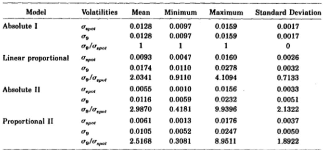
In Tables IV and V we report the estimation results for the spot-rate and forward-rate models, respectively. Before discussing the results, we point out that the estimates for the nine-year forward-rate volatilities reported in
Comparison of Models for Valuing Interest-Rate Options 289
TableIV
Estimated (Absolute) Volatilities of the Spot and Nine-Year Forward Rate for the Forward-Rate Models
This table presents the estimated (absolute) volatiJities of the spot and nine·year forward rate for the forward-rate models. Absolute I is the one-factor model with constant volatility. Linear proportional denotes the one-factor model with linear proportional volatility. Absolute 11 is the two-factor model in which both volatility functions are independent of the levei of the forward rate. In the two-factor model Proportional lI, both volatility functions are proportional to the leveI of the forward rate. The parameters ",po, and ". are the (absolute) volatilities of the instantaneous spot rate r(t) = ((t,t) and the instantaneous nine-year forward rate ((t,t + 9) implied by the different models. Ir multiplied by 100, they represent volatilities in percent p.a. The parameters are estimated for 204 Fridays within the valuation period from January 5,
1990, through November 16, 1993.
Model Volatilities Mean Minimum Maximum Standard Deviation
Absolute I u.pot 0.0128 0.0097 0.0159 0.0017
".
0.0128 0.0097 0.0159 0.0017Ug/utlPot 1 O
Linear proportional aspa' 0.0093 0.0047 0.0160 0.0026
".
0.0174 0.0110 0.0278 0.0032Ug/utlPuI 2.0341 0.9110 4.1094 0.7133
Absolute 11 u spot 0.0055 0.0010 0.0156 0.0033
".
0.0116 0.0059 0.0232 0.0051"glu.pal 2.9870 0.4181 9.9396 2.1322
Proportional 11 uspot 0.0061 0.0013 0.0176 0.0037
".
0.0105 0.0052 0.0247 0.0050Ug/utJpot 2.5168 0.3081 8.9511 1.8922
Table IV are not comparable to the estimates for the nine-year zero-rate
volatilities of Table V. The nine-year forward-rate volatility refers to an
in-stantaneous forward rate maturing nine years from the current day. The latter refers to a rate for a period that is nine years long. Only the
instan-taneous volatility of the spot rate r(t)
=
f(t, t) is comparable across alI models.If uspot and Ug are multiplied by 100, we obtain the (absolute) volatilities
in percentage per annum (p.a.). A division of uspot , as estimated for the
absolute model by an average short rate of 0.088 in the valuation period, results in an approximation for the mean relative volatility of about 15 per-cent p.a.
On average, the volatilities of the forward rates increase with maturity. The only exception is the absolute one-faetor model in which constant vola-tilities are assumed. The (constant) volatility of this model is approximately
equal to the arithmetic mean of uspot and Ug in the linear proportional mode!.