Essays on the monetary aspects of the term structure of nominal interest rates

Escola de

Pós-Graduação

em

Economia

- EPGE

Fundação

Getúlio

Vargas

ESSAYS

ON

THE

MONETARY

ASPECTS

OF

THE

TERM

STRUCTURE

OF

NOMINAL

INTEREST

RATES

Tese

submetida

à Escola

de

Pós-Graduação

em

Economia

da

Fundação

Getúlio

Vargas

como

requisito

de

obtenção

do

Título

de

Doutor

em

Economia

Aluno:

Ricardo

Dias de

Oliveira

Brito

Escola de

Pós-Graduação

em

Economia

- EPGE

Fundação

Getúlio

Vargas

ESSAYS

ON

THE

MONETARY

ASPECTS

OF

THE

TERM

STRUCTURE

OF

NOMINAL

INTEREST

RATES

Tese

submetida

à Escola

de

Pós-Graduação

em

Economia

da

Fundação

Getúlio

Vargas

como

requisito

de

obtenção

do

Título

de

Doutor

em

Economia

Aluno:

Ricardo

Dias

de

Oliveira

Brito

Banca

Examinadora:

Professor

Renato

Galvão

Flores

Jr.

(Orientador)

Professor

Afonso

Celso

Pastore

(EPGE)

Dr.

Franklin

Gonçalves

(BBM)

Professor

Márcio

Garcia

(PUC-Rio)

Professor

Wolfgang

Bühler

(Manhein)

Agradecimentos

Esta tese conclui meus programas de mestrado e doutorado iniciados em 1995 na

EPGE/FGV. Ao longo dos 6 anos e meio, algumas pessoas e instituições foram

fundamentais para que tenha persistido numa jornada que por vezes pareceu equivocada

ou sem fim.

Meu orientador Renato Flores Jr. avalizou todos meus projetos com inesgotável

e cúmplice paciência.

Os professores Marco Antônio Bonomo e Fernando de Holanda Barbosa foram

mais que mestres. Muito acessíveis, estimularam minha auto-confiança, incentivaram a

criatividade e patrocinaram o início da minha carreira acadêmica.

Os funcionários e demais professores da EGPE ofereceram o suporte necessário

para o estudo e a pesquisa, e a rede de financiamento CAPES, CNPq, BBM e FGV

funcionou com eficiência para que não faltassem recursos durante o programa.

Os colegas de doutorado Carlos Hamilton Araújo, Joísa Saraiva, Osmani

Guillen, Márcia Leon, Marcos Tsuchida e Mônica Viegas proporcionaram um ótimo

ambiente de trabalho. Sempre disponíveis para discussões técnicas ou conversas amigas,

foram uma grande fonte de idéias e incentivos.

Os amigos Flávio Cunha, Felipe Pianetti, Fernando Rocha e Sérgio Xavier foram

minha família no Rio de Janeiro.

No ano que passei na Universidade de Chicago, Ruy Ribeiro me recebeu com

inigualável hospitalidade. Me acolheu como um amigo antigo e merecedor de sua

confiança para compartilhar trabalhos acadêmicos e explorar temas para pesquisa.

Cristiana dividiu comigo toda a angústia da tese. Foi confidente, foi conselheira

e foi, sobretudo, privada de convivência. Sem o seu apoio, o trabalho teria sido mais

difícil. Merece carinhosos agradecimentos.

Mais que o fim de um programa de doutorado, esta tese conclui um projeto de

educação formal. Neste programa mais longo, Márcia e Maurício sempre foram amigos

solidários, mestres incentivadores e financiadores generosos. Foram pais exemplares,

sem os quais esta jornada seria impossível.

Rio de Janeiro, 5 de Setembro de 2001

À Márcia

e Maurício

Brito,

índice

Introdução 1

Capítulo 1: Stochastic Growth and Monetary Policy: the impacts on the term

structure of interest rates 9

Capítulo 2: A Jump-Diffusion Yiel-Factor Model of Interest Rates 58

Capítulo 3: What the short-term interest rate can do for mean-reverting

Essays

on

the

Monetary

Aspects

of

the

Term

Structure

of

Nominal

Interest

Rates

Ricardo D. Brito

October 4, 2001

1

Introduction

Interest rates are key economic variables to much of finance and

macroeco-nomics, and an enormous amount of work is found in both fields about the

topic. Curiously, in spite of their common interest, finance and macro research

on the topic have seldom interacted, using different approaches to address its

main issues with almost no intersection. Concerned with interest rate

contin-gent claims, finance term structure models relate interest rates to lagged interest

rates; concerned with economic relations and macro dynamics, macro models

regress a few interest rates on a wide variety of economic variables. If models

are true though simplified descriptions of reality, the relevant factors should be

captured by both the set of bond yields and that of economic variables. Each

approach should be able to address the other field concerns with equal emciency,

since the economic variables are revealed by the bond yields and these by the

However, models are also approximations that choose a subset of states to

imperfectly capture the full set of factors. The set of yields and the set of

economic variables do not capture the same factors nor give the same relative

importance to each factor. Indeed, financial models have not accomplished to

properly incorporate macro variables, despite the belief that their changes are

major sources of changes in the shape of the yield curve. Macro models, on

the other hand, have not accomplished to properly incorporate the yield curve,

despite the belief that their shape is an indicator of economic conditions.

Many stylized facts still challenging established theory may find explanation

in this largely unexplored complementarity. Some that deserve mention are:

(i) the pro-cyclical pattern of the levei of nominal interest rates (Fama &

French [33]);

(ii) the countercyclical pattern of the term spread1, as well as the low

sen-sitivity of long yields to monetary policy changes (Fama & French [33] and

Thornton [66]);

(iii) the pro-cyclical pattern of the curvature of the term structure;

(iv) the lower predictability of the slope of the middle of the yield curve

(Campbell, Lo & MacKinlay [18]);

(v) the negative correlation of changes in real rates and expected inflation

at short horizons (Campbell & Ammer [17] and Barr and Campbell [10]);

(vi) almost ali variance of the yields can be explained by three unknown

factors that impact on the levei, slope and curvature of the term structure

lrThe term spread is defined as the difference between the yield-to-maturities of a long and

(Litterman &. Scheinkman [43]);

(vii) the high sensitivity of the volatility of the short-rate change to leveis

(Chan et ai [19]);

(viii) the low predictability of the short-rate changes (Chan et ai. [19]);

(ix) the overreaction of the short-term rate;

(x) the leptokurtosis of the density of the yield changes at high-frequency

data.

This thesis intends to be a contribution to the integration of the finance

and the macro theories of interest rates. The three essays address monetary

aspects of the term structure of nominal interest rates. Along them, the

dis-continuous setting of the nominal short-rate by the monetary authority plays

a crucial role. Either explicitly or implicitly, the monetary authority forces the

left-end of the term structure to match an exogenously specified levei through

discontinuous changes of the short-term nominal interest rate. Given that the

monetary authority is constrained to keep inflation close to zero, future changes

in the controlled rate can be forecasted by looking at the dynamics of the

ex-pected inflation and may be incorporated into the shape of the term structure.

In the remaining of this section we briefly summarize the three papers.

1.1 Stochastic Growth and Monetary Policy: the impacts on

the term structure of interest rates

This paper builds a simple intertemporal optimization model with staggered

prices a Ia Fuhrer & Moore [35], investment costs and a policy rule for setting

cyclical patterns of the term structure of nominal interest rates.

Neutral interest rate is formally defined and the net disinvestment on bonds

is proposed as a microeconomics foundation for the excess demand term that

appears in the Fuhrer & Moore's [35] sticky inflation equation. Fixed by the

policy rule:

k+-\ =k + vt,

{0

eTwTTÍ with probability ç |tt£_i |

is the monetary policy shock, 7T(_i is the last period inflation, and e and ç are

positive constants, the nominal short-rate process combines with the inflation

stickiness assumption to break monetary policy neutrality. The resulting model

is able to explain the following stylized facts:

(i) pro-cyclical pattern of the levei of nominal interest rates;

(ii) countercyclical pattern of the term spread;

(iii) pro-cyclical pattern of the curvature of the term structure;

(iv) lower predictability of the slope of the middle of the yield curve; and

(v) negative correlation of changes in expected inflation and real rates at

short horizons.

The model extends Balduzzi, Bertola & Foresi's [8], Rudebusch's [62], Tice

& Webber's [67] and Piazzesi's [60] analyses of the monetary policy impacts on

the term structure in the sense that it is done in an intertemporal optimization

1.2 A Jump-Diffusion Yield-Factor Model of Interest Rates

This paper builds a two yields-factor model of interest-rate derivatives pricing,

which is applied to the U.S. Treasury nominal zero-coupon bonds. The two

yields chosen are the Federal Fund Rate Target and the one-year yield, what

allows to separate the monetary policy risk from the remaining macroeconomic

risk.

The Federal Fund Rate Target is shown to be a Poisson process, given

the expectations of the macroeconomic conditions incorporated in the one-year

yield. The one-year yield is parametrized to result in a consistent model, in

accordance with Duffie and Kan [28].

Given the two states, the model adjusts well to the U.S. average yield curve

and to the actual yield curve from January 1990 to December 2000.

Further-more, (vi) almost ali variance of yields can be described in terms of the one-year

yield, the Federal Fund Rate Target and their spread, respectively shown to

impact on the levei, the slope and the hump of the term structure of nominal

interest rates.

The model is a simple alternative to Babbs & Webber [6], Attari [5], El-Jahel

et ai. [30], Duffie et ai. [29], Piazzesi [58] and Das [25].

1.3 What the short-term interest rate target can do for

mean-reverting modelling

This paper shows that the bad fit of univariate constant-mean-reverting

is due to the omission of its target, discontinuously set by the Federal Open

Market Committee. With a constant long run mean, neither the levei volatility

models like Chan et ai. [19], nor the stochastic levei volatility models suggested

by Brenner et ai. [13] are able to explain the rate changes or the squared rate

changes. The variable-mean-reverting diffusion process that combines the rate

target as the long-run mean with the stochastic levei volatility results in an

improved fit and forecasts a considerable proportion of both changes.

The puzzling (vii) Chan et al.'s [19] high sensitivity of the volatility of the

short-rate change to leveis shrinks; while (viii) the predictability of the

short-rate changes improves, (ix) The apparent Federal Fund Rate overreaction is

also solved. Because the rate target is generated by a jump process and the

volatility seems to be of the stochastic levei kind, (x) the density of yield changes

are not normally distributed and fatter tails are justified. Furthermore, weak

evidences are produced that the rate target might outperform the Federal Fund

Rate as a short-term factor in term structure models.

The model extends Chan et ai. [19], Brenner et ai. [13] and Hamilton [37]

specifications.

2

Conclusion

and

Extensions

Understanding the monetary aspects involved in the term structure of nominal

interest rates seems to payoff in improved ability to explain the interest rate

dynamics as the three essays of this thesis have shown. Represented by the

leveis of abstraction: in a complete economy model like Stochastic Growth and

Monetary Policy, in a more specific asset pricing model like A Jump-Diffusion

Yield-Factor Model of Interest Rates, or in a specific parametrization of the

stochastic process followed by the short-rate like What the short-term interest

rate target can do for mean-reverting modelling.

The usual list of extensions necessary to give research some credibility apply

to ali three papers. Other empirical experiments may show how good are the

proposed models to fit various sets of data, in and out of the sample. The

relative importance of the individual hypotheses to generate the model results

deserve explicit study and the testable hypotheses should be checked.

Each paper also suggests particular extensions. In Stochastic Growth and

Monetary Policy, different sets of parameters can be simulated and,

alterna-tively, the set of parameters can be fully estimated. The model's speed of

ad-justment and length of the cycles should be compared with the observed ones.

The usual confrontation of the model generated dynamics with the dynamics

implied by an unrestricted VAR also deserves mention. Given that expansions

are longer than recessions, the introduction of some asymmetry may improve

the actual fits.

In A Jump-Diffusion Yield-Factor Model of Interest Rates, the comparison

with other bond pricing models may give an idea of the model relative efficiency.

How good are out of the sample predictions is also an important complementary

exercise.

In What the short-term interest rate target can do for mean-reverting mod

of the proposed process to the empirical one guiding the choice. However, rather

than local improvements as alternative GARCH specifications, it is thought that

the results in this and the previous papers point out the clear need of

abandon-ing the univariate set-up and using multivariate diffusions models to address

Chapter

1

Stochastic

Growth

and

Monetary

Policy:

the

impacts

on

the

term

structure

of

interest

rates

October 5, 2001

Abstract

This paper builds a simple, empirically-verifiable rational expectations

model for term structure of nominal interest rates analysis. It solves a

stochastic growth model with investment costs and sticky inflation,

sus-ceptible to the intervention of the monetary authority following a policy

rule. The model predicts several patterns of the term structure which

are in accordance to observed empirical facts: (i) pro-cyclical pattern of

the levei of nominal interest rates; (ii) countercyclical pattern of the term

spread; (iii) pro-cyclical pattern of the curvature of the yield curve; (iv)

lower predictability of the slope of the middle of the term structure; and

(v) negative correlation of changes in real rates and expected inflation at

short horizons.

JEL classification: E32; E43; E52

Keywords: Controlled Short Rate; Discontinuous Changes; Nominal

1

Introduction

This paper provides an answer to two apparently unrelated questions:

How can an intertemporal equilibrium model adequately fit an arbitrary

exogenous term structure of interest rates?

What is the role of monetary policy in determining the term structure of

interest rates?

On the first issue, intertemporal general equilibrium modelling of interest

rates still leaves many questions unanswered. As an example, scalar

time-homogenous afiine equilibrium models1, that provide tractable and rich analytic

results with terse description of an equilibrium economy, are intrinsically

inca-pable of fitting an arbitrary exogenous term structure because of their constant

levei of reversion. Worse, when tested against more general scalar

specifica-tions, they are usually rejected, suggesting either the existence of nonlinearity

or of omitted variables (Chan et ai. [19] or Ait-Sahalia [3]).

On the second issue, despite the belief that changes in the monetary pol

icy impact on asset returns in general2 and are a major source of changes in

the

shape

of the

yield

curve3,

micro-financial

models

have

not

accomplished

to

properly incorporate it yet. The neglect to deal with macro links leaves

unex-plained, certain stylized facts like the pro-cyclical nominal interest rate leveis,

the countercyclical term spread (Fama & French [33]), or the negative short-run

'The univariate version of Cox, Ingersoll and Ross [24] can be seen as the most important

member of the class.

2 For example, Thorbecke [65] and Patelis [56] document the existence of a monetary risk

premium and show the role of monetary policy in the predictability of the asset returns.

correlation between expected inflation and the expected future real interest rate

(Campbell & Ammer [17] and Barr & Campbell [10]).

As macro links, omitted variables and constant reversion leveis seem to

be the weak points of the scalar time-homogeneous equilibrium models, an

attempt is made here to incorporate a macro monetary policy variable into

an intertemporal equilibrium model. The goal is to get a simple,

empirically-verified rational expectations model for the term structure of nominal interest

rates. A model which allows great flexibility in the changes of the yield curve,

in response to changes in the macroeconomic environment.

We portray the character of fluctuations in the term structure of nominal

interest rates, inflation and aggregate output with staggered price contracts

and investment costs, subject to technology shocks and expectational errors

by price bargainers. We end up solving a stochastic growth model, subject

to investment costs and sticky inflation similar to Fuhrer [34], but susceptible

to the intervention of an externai authority. The intertemporal optimization

implies a complete description of the multi-period expected returns, and the

model allows the derivation of a nominal term structure which incorporates the

effects of monetary policy. Through discontinuous changes of the short-term

nominal interest rate, the Central Bank forces the left-end of the term structure

to match an exogenously specified levei. This implies a non-zero net supply of

nominal riskless bonds and adds the possibility of jumps in ali forward-looking

variables. Given that the monetary authority is constrained to keep inflation

close to zero, future changes in the controlled rate can be forecasted by looking

shape of the term structure.

The resulting model extends Balduzzi, Bertola & Foresi's [8], Rudebusch's

[62], McCallum's [47], Tice k Webber's [67] and Piazzessi's [60] analyses of

the monetary policy impacts on the term structure in the sense that, in an

intertemporal equilibrium framework, it allows the joint explanation of more

stylized facts. Indeed, with a relatively simple model it is shown that the mon

etary policy has real effects. We eventually explain: (i) the pro-cyclical pattern

of the levei of nominal interest rates; (ii) the countercyclical pattern of the

term spread4 (as well as the low sensitivity of long yields to monetary policy

changes); (iii) the pro-cyclical pattern of the curvature of the term structure;

(iv) the lower predictability of the slope of the middle of the yield curve; and

(v) the negative correlation of changes in real rates and expected inflation at

short horizons. Though empirical evidence on these facts is abundant in the

literature (see for example, Campbell, Lo & MacKinlay [18], Fama & French

[33], Rudebusch [62] and Barr and Campbell [10]) no simple model exists

tak-ing simultaneously into account ali them. Moreover, implications of the here

developed model can be explored in a bond pricing context.

The paper has the following structure. Section 2 presents the empirical

patterns, while section 3 reviews the term structure pattern implied by the

plain Real Business Cycle model and points out its nominal indeterminacy.

Both act as a motivation to section 4, where the proposed model is explained in

a representative agent framework. Examples and simulations are performed in

4 The term spread is defined as the difference between the yield-to-maturities of a long and

section 5, and section 6 concludes. The equivalence between the representative

agent and the competitive formulation of the model is fully shown in Appendix

1; Appendix 2 explains the numerical method used in the simulations.

2

Some

Stylized

Facts

This section presents empirical evidences on the movements of the term

struc-ture of nominal interest rates, inflation and output, to which the numerical

predictions of the theoretical models will be subsequently compared. The em

pirical pattern of the term structure is reproduced below using the interest

rate data available at the FED of Saint Louis' web site (www.stls.frb.org/fred),

which are taken from the H.15 Release by the Board of Governors. The seven

rates chosen were: 3-Month Treasury Bill Rates (TB3m), 6-Month Treasury Bill

Rates (TB6m), 1-Year Treasury Bill Rates (TB1), 3-Year Treasury Constant

Maturity Rate (CM3), 5-Year Treasury Constant Maturity Rate (CM5), 7-Year

Treasury Constant Maturity Rate (CM7), 10-Year Treasury Constant Maturity

Rate (CM10). T-Bills are secondary market rates on Treasury securities and

the CM rates are constant maturity yields.5.

For B\, the nominal price at t of the purê discount j period bond (or the

zero coupon bond that matures in j periods from t), the yield-to-maturity, yf,

is the per period interest rate accrued during the j periods:

°The results to be presented below hold for the Fama k, Bliss data set as well, that uses

only fully taxable, non-callable bond. The monthly data contain one to five years-to-maturity

bonds and cover the period from July 1952 to January 1998, providing 547 observations. The

Fama and Bliss data set was constructed by Fama and Bliss [32] and was subsequently updated

by the Center for Research in Security Prices (CRSP). The results can be made available

what means the yield-to-maturity is the average return on the bond held until

maturity.

Because B\ is known at time t, yf is the j period riskless nominal rate

prevailing at time t for repayment at t + j. The one period riskless nominal

rate prevailing at time t for repayment at t + 1 deserves special notation, it:

and is denoted the spot interest rate. For j > l, the l period nominal holding

return of the j period bond between t and t + l, h3t+l t, is the per period

interest rate accrued during the / periods:

Given the consumer price index at t, Pt, and the inflation between t and

t + l, ftt+i, t = -^ lj the l period real holding return of the j period

nominal bond, rlt+í t, can be analogously defined as:

Note that both rJt+l t, itt+i, t and h3t+l t only become known at t +1.

(ro). They were transformed to yield-to-maturity by respectively: y3' = (1 +

°tbe\ * ioõ)^ 1 and y3' = (1 ru * iqõ) * 1, where j is time-to-maturity in

years. Ali yields below will be expressed in annualized form.

2.1 Pro-cyclical nominal interest rate leveis and countercyclical

term spread

The evolution of the yields-to-maturity of the three-month and of the ten-year

bonds are plotted in Figure 1 with shades added to mark the business cycles.

Every white period points one expansion cycle from trough to peak, as classified

by the NBER. The gray periods mark the contraction periods from peak to

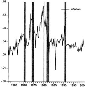
trough. The (i) pro-cyclical pattern of the levei of interest rates is clear: the

levei increases during expansion and decreases during contraction. This may

be related to the pro-cyclical pattern of the inflation levei, as shown in Figure

2.

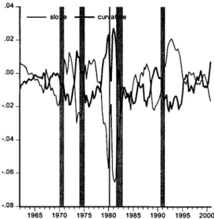
Figure 3 shows the evolution of the slope and the curvature of the yield

curve

6.

The

(ii)

term

spread

presents

a countercyclical

pattern:

the

slope of

the yield curve is big at the trough and decreases during the cycle to become

small at the peak. (iii) Curvature seems to decrease along contractions (shades)

and to increase during expansions.

From (i), (ii) and (iii), it results that the mean term structure at the trough

is a positive sloped, relatively steeper, concave curve, while the mean term

structure at the peak is a negative sloped, relatively flatter, convex curve.

6 The slope of the yield curve is nothing more than the term spread (CM10 TB3m). The

2.2 Lower predictability of slope of the médium term rates

In the analysis of the term structure, the many versions of the Expectation

The-ory of the term structure of interest rates have played an important role. Loosely

stating, the Expectation Hypothesis says that the expected excess returns on

long-term bonds over short term bonds (the term premiums) are constant over

time. This means the term premium can depend on the maturity of the bonds

but

not

on time:

Et \h3t+l

t - h^+l

t] = f (j, k, l), with

% = 0 V j > k > l

7. In its

Purê

version

(the

Purê

Expectation

Hypothesis,

PEH),

it imposes

the

term premium to be zero.

If any version of the Expectation Hypothesis holds, the slope of the yield

curve is able to forecast interest rate moves, and this predictability is uniform

along ali maturities. For example, to test such a predictability for the

"one-period return", the PEH reduces to check whether the slope, 6, of the regression:

4:í - vi) = a + &jry

(v\ - ví)

is significant. Indeed, the above hypothesis implies that 6 = 1 for every l.

Using monthly zero-coupon bond yields over the period 1952:1 to 1991:2 8,

Campbell, Lo & MacKinlay [18] estimated equations similar to (1) for 2 to 120

months and got the results shown in Table 1.

Besides the ò's being statistically different from 1, the stylized fact that their

results bring to scene is the U-shaped pattern of these slope coefficients: the

7The Expectation Hypothesis can be stated in real or in nominal terms.

forecasting power diminishes from the one month to the one year case and then

increases up to the ten years case. This means that (iv) the predictability of

the middle of the yield curve is lower than those of the edges.

2.3 Principal component analysis

Are the previous four stylized facts the result of some identifiable factors? In

this regard, principal component analysis might point at least how many factors

are relevant for empirical term structure motion. Table 2 shows factors with a

pattern similar to the one uncovered by Litterman & Scheinkman's [43].

The first factor has the same sign in ali bonds but, different from Litterman

& Scheinkman, its impact is higher on the shorter ones. This gives a different

interpretation, that the first factor causes moves in the leveis and in part of

the slope changes. The second factor changes sign from the short end to the

long end of the maturities, which means it causes the changes in slope. Finally,

the third factor, which has more impact at the short and long ends of the term

structure, is interpreted as the curvature factor.

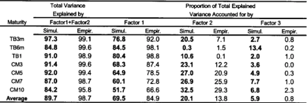
Table 3 shows the proportion of total variance explained by the three factors.

In the FRED data, the first two factors explain most of the movements and

almost nothing is left to factors 3 and further 9.

Using the FRED 1969-2000 sample and varying frequency, we have

per-formed other principal component analyses (not shown) and obtained that,

9Litterman & Scheinkman [43] used weekly observations, from January 1984 to June 1988,

of maturities 6-month, 1, 2, 5, 8, 10, 14 and 18-year. They got averages of 89.5 %, 8.5 % and 2

% for the proportion of the total explained variance by the first three factors. Their different

result might have been caused by the different frequency and length of the time series, or span

once frequency is increased, the first factor loses explanatory power to the

sec-ond and third ones. This is a weak evidence that the 2nd. and 3rd. factors are

more important in explaining short run movements 10.

2.4 Negative correlation of changes in real rates and expected

inflation at short horizons

Well known in the fixed income theory is the Fisher hypothesis that there is no

correlation between the expected inflation and the real interest rates: nominal

interest rates change to fully compensate for expected inflation variations.

However, this hypothesis is not verified once taken to data: (iv) there exist

negative correlation between expected inflation and real interest rate at short

horizons. This fact is shown for example by Barr and Campbell [10], who,

working with U.K. data, find correlations of changes in real rates and expected

inflation of-0.69, -0.06 and-0.08 for 1-year, 5-year and 10-year, respectively11.

The significant negative correlation got at a short horizon is puzzling, since it

is expected that investors increase (decrease) their asked nominal interest rates

every time a higher (lower) inflation is expected.

10This is also an evidence that L&S different results might have been caused by the different

length of the time series or span of the maturities.

11 Campbell & Ammer [17] and Pennacchi [57] find the same evidence using respectively

3

ASimple

Intertemporal

EquilibriumTheoryof

the

Term

Structure

with

production

Because intertemporal optimization models imply a complete description of the

multi-period expected returns, and the term structure of interest rates is merely

the plot of these observed returns, they are suitable as the microfoundation of

a term structure model, as shown by Cox Ingersoll and Ross [23].

In the Real Business Cycle (RBC) model with labor supplied inelastically,

the representative agent maximizes:

(2)

i = t

with: u'(.) > 0, u"(.) < 0; subject to the budget constraint:

3 = 2

7Tt,t-i)

to the technology shock AR(1) dynamics:

(3)

-Tf,

N(0,o*);

(4)

and the transversality conditions:

lim

13%

= 0;

where:

c stands for real consumption;

k is the real capital stock;

0 is the productivity shock;

0 < a < 1 is the capital elasticity12;

6 is capital depreciation;

(1 + 7Tt,t-i) = -p-j^ is the infiation between í 1 and t, with the price index

Pt not known before í;

(1 + it) is the nominal interest rate of the one period bond held between

í 1 and t, known at t 1;

B3t is the nominal price of the j period bond;

òj is the quantity of the bond the consumer carries from í 1 to í, and j is

the number of periods to maturity;

ò° is the

quantity

of the

bond

redeemed

at t;

and Tt are real taxes.

Because labor is inelastically supplied, the production function is presented

in terms of per-capita capital, and the above formulation couches the case of

a constant return-to-scale production function. Also, to make presentation

lighter, instead of the usual normalization of nominal unit price at maturity,

12The production function f (k,0) = dtkf presents the usual conditions:

/i () > 0, h (.) > 0, / (.) < 0, /, (0,.) = oo, h (oo,.) = 0;

B®

= 1 V t, we

assume

that

the

next-to-mature

bond

costs

one

nominal

unit

and is worth (1 + ít+i) nominal units at redemption.

From the above, the representative agent value function can be posed as:

V

[kt;l4;j>0;

₍₇₎

max

c, k, b

-At

2 -(1-6) kt

and solved to result in the agenfs optimal allocation rules:

v! (et)

= f3Et

{ [adt+,k?J

+ (1 - 6)]

u' (cí+1)}

₍₈₎

and

u' (ct)

7Tt+1,t)

Vj;

(9)

(10)

taking prices as given.

Recursion on (10) and the law of iterated expectations implies the lperiod

1 = _Pt+i Pt u'(ct+l) _u'(ct)

(11)

and gives the whole real term structure implied by the model.

Inasmuch as the yield-to-maturity of every lperiod bond (y[) is known for

certainty

at t, (l + ylt)

= -gr,

it can

be

taken

out

of the

expectation

operator,

resulting in:

1

B>

t u'(ct) Vi; (12)

that provides the whole nominal term structure.

It is trivial

that,

for

l = 1, yj

= it+Y,

and

the

above

formula

simplifies

to:

1 =

_rt+1,

_{t) -^}

₍₁₃₎

where the spot rate it+-\ can be put outside the expectation if desired.

From (12), again by use of the law of iterated expectations, we obtain:

Covt u'(ct+l)

;, t u'{ct)

(14)

Vi;

Equation (14) means the PEH holds only in the spedal cases where the risk

premium is zero.

Also, working on (12), results in the generalized "one-period return" PEH:

(15)

Covt

as called by Campbell, Lo and MacKinlay [18]. Again, only when the risk

premium is zero, does the "one-period" PEH hold.

The agenfs optimal conditions allow us to define:

u' (ct)

as the stochastic discount function (or the pricing kernel); which in the present

model is equivalent to the intertemporal marginal rate of substitution in

con-sumption.

3.1 Equilibrium without externai intervention: inflation and

nominal interest rate indeterminacy

An equilibrium sequence is defined as a set of stochastic vectors

ct, it+i,

Kt,t--\,

rl+i,v

frt+i>

Tt)

satisfying

the

f.o.c.'s

and

the

Without externai intervention, the exogenous supply of bonds is zero:

as well as taxes rt = 0, and, given (4), the consumers' decision simpliíies to

split wealth between capital and consumption by obeying (8) and the simplified

budget constraint:

(17)

for every t.

The initial capital stock, the technology dynamics (4), and the

transversal-ity condition (5) define the saddle path expected to be followed by (fc , c) in the

system (8) and (17). Substitution of (17) into (8) defines a stochastic difference

equation in k that, given the initial capital stock, initial technology and (5),

obtains the optimal capital path (fc*) and provides the inputs to obtain the

optimal consumption path (c*) by (17). The above hypotheses are enough to

guarantee that the distribution of optimum aggregate capital converges point

wise to a limit distribution when returns are decreasing: fc is pushed to the levei

kss where the expected marginal productivity of capital equals the rate of time

preference:

afc"s~1

6 = (1//3)

- 1 . When

returns-to-scale

are

constant,

they

are as well enough to guarantee that the rates of growth converge pointwise to

a limit distribution13.

The application of {C(}^0 to (11) endogenously determines the expected

/ period real returns on a j period nominal bonds from t to t + l:

and gives the whole expected real term structure implied by this equilibrium.

We now define what we understand by neutral values.

Definition 1 At any time t, the endogenous variables values are neutral,

de-noted

(*£,,

cf,

i?+,,

h?+(v

<1)t,

r?+lt,

bfjt+^,

when

the

real

stock

of

bonds is fully rolled over with no portfolio rebalance:

This means that we qualify ali interest rates as neutral when they are

ob-tained without changes in the bonds' maturity profile. There is no net externai

intervention, in the sense that the debt-credit profile is kept constant. Thus,

within a period, the neutral values are nothing more than those for which the

private sector's net demand for every maturity bond is zero, what means people

do not sell bonds to finance capital or the other way around.

Because there is a stochastic shock in the production function, the neutral

real spot rate nuctuates around a trend defined by the optimal capital path.

For example: if kt is increasing along time and the production function presents

decreasing returns-to-scale, the productivity trend is decreasing and real neutral

rate is expected to decrease as the economy tends to the steady state.

completely defined by (4), (8), (17) and (5). Equation (13) is nothing more than

the Fisher relation that defines next period inflation given the spot nominal

interest rate, or the other way around. Because the expected spot real interest

rate is completely determined by the real factors and is every time the expected

marginal productivity of capital, expected inflation sensitivity to the levei of

the nominal interest rate is one, what means no correlation between nominal

and real variables.

Although the inflation and nominal rate indeterminacies are a consequence

of having more variables than equations, the inclusion of a cash-in-advance

restriction or a fiscahst-theory type of reasoning does not change the above

conclusions. Due to this one-to-one correspondence between i and n, there is

no cyclical pattern (i) in the levei of the nominal term structure, (ii) or in that

of the term spread, (iii) or in that of the curvature. (iv) The predictability

of the slope of the yield curve is good and equally credible for every maturity.

Moreover, (v) there is no correlation between expected inflation and the real

interest rate since the real interest rates vary with the marginal productivity of

capital and the Fisher hypothesis holds.

Summing up, system (4), (8), (17) and (5) alone does not split the changes

in the nominal rate into changes in the real rate and inflation, and is not of

great use in explaining how monetary policy affects real activity and inflation.

Basically, it assumes neutrality (and superneutrality) and thus thwarts the

pos-sibility that nominal interest rate and inflation vary independently. Quite

un-realistic, inflation reduction to zero can be done in one painless down-move of

on the real activity.

Notwithstanding, there exists one degree of freedom in the above model to

couch an ad hoc assumption, and this is done, in conjunction with inílation

stickiness, in section 4.

4

The

Model

The proposed model describes a closed economy 14 with firms and capital

ac-cumulation, subject to investment cost and staggered price contracting, and

susceptible to the intervention of a monetary authority. For presentation

pur-poses, we develop the main ideas in the representative agent framework. The

equivalence with a more detailed economy, where consumers and firms interact

in a world of staggered price contracting, is shown in Appendix 1.

4.1 The Real Side with investment costs

The representative agent maximizes (2), subject to a budget constraint slightly

different from (3):

= 6tk? + (1 - 6) kt +

(l+7Tt)t_i)

14As pointed in Meltzer [49] pp.50, in an open economy, the exchange rate would be just

one more of the many relative prices in the transmission process, without altering the basic

and

to (4), (5), (6);

where:

<p (^- -

l\

is the

cost

of adjustment,

and

the

other variables have the previous stated meaning.

Now, the representative agent value function can be posed as:

V (kt-M;

j > 0;6t)

max <

c, k, b

-A,

-etk? - (i

and the solution is similar to the one in section 3, except that:

replaces (8).

4.2 Contracting Specification and the Inflation Dynamics

Once accounted the investment costs, it is assumed that consumption and cap

ital goods (c and k) are the same final good, which is the aggregation of two

differentiated goods produced, consumed and invested together in a fixed

pro-portion of half each. Although undesirable, the no substitutability between

these (differentiated) component goods simplifies matters and buttresses a

gered price contracting similar to Fuhrer & Moore [35]. In our paper, agents

negotiate the nominal price contracts of the two final goods, that remain in

ef-fect for two periods. As the model hypothesizes that production, consumption

and investment are split between these two goods, the aggregate price index at

t is defined as the geometric mean of the contract prices:

x x

Pt = Xz X2 - (í)c>\

where:

Xt is the contract price

and Pt is the aggregate price index at t.

Agents set nominal contract prices so that the current real contract price

equals the average real contract price index expected to prevail over the life of

the contract, adjusted for excess demand conditions:

xt

(23)

where the excess demand term Yt was parametrized as Yt = eyt. With this, yt

is the excess demand which can be calculated from the budget constraint (19)

as:

Vt =

fct+1+^(^l-l

3 = 2

- (etk? + (i

í

(l + 7rtlí_i)

Considering the expression after the first equality signal, the two first members

describe total demand for goods, while the last one (the big expression between

brackets) is the supply of goods. Thus, excess demand can be read as the

private sector's net demand for bonds, and there is no excess demand (yt = 0)

when variables from t to t + 1 are neutral (as stated in the Definition).

Equation (23) causes the inflation dynamics:

(1 + 7rí)t_i)

= (1 + 7rt_1,í_2)5

(1 + Et [7rt+lit])*

(YtYt^ynt,

(25)

where Qt = eWf is the expectational error orthogonal to date í 1 information

set, and allows inflation stickiness in the present model. Note that if expressed

in log terms, (25) gives an expression very similar to the one in Fuhrer íc Moore

[35], which will be used in the simulations in section 5 below.

4.3 The Monetary Authority Intervention and the Role Played

by Money

Since we are interested on the study of moves in the yield curve, and not on the

study of optimal monetary policy rules, we don't care about objective functions

of the monetary authority and related issues. It is enough that the monetary

authority be concerned about inflation, have funds to intervene in the bond

market, and knows its dynamics is given by (25). This being the case, it is

prone to control the one-period spot interest rate to fight inflation. Due to

operating constraints, it is assumed, without loss of generality, that it uses the

«t+1 =k + vu (26)

where:

!0,

probability :

and e and ç are positive constants 15.

In other words, the spot rate tends to remain constant from period to period,

except for jumps whose probability is an increasing function of the inflation

levei. If inflation is positive the eventual jump is positive, and if inflation

there is deflation the jump is negative. When inflation grows, the probability

of jumps increases and so the expected value of the next period spot rate.

Because inflation is persistent, policy only reverts when the inflation target has

been mostly reached.

The key to our model is monetary authority behavior in the bond market.

It acts buying or selling one-period bonds that pay riskless nominal interest

rate (1 + it+i), but risky real interest rate:

it+i

revealed at t +1. Besides, the authority runs no déficit, what forces it to charge

the individuais a lump sum tax to payoff the net interest:

15 (26) implies the monetary authority inflation targeting is zero. This assumption can be

t°ví>o'

(27)

where bf stands for the per capita bond demand.

As individuais receive the full proceeds of bonds they hold and are charged

lump sum, they choose to long or short the one-period bond once its real

ex-pected return diverges from the expected neutral rate. Thus, although lending

to or borrowing from the monetary authority are just simple storage in the

aggregate, non-zero net demand for one-period government bonds shows up due

to the non-cooperative individual behavior induced by the tax system.

Not only the above rule makes it easy to forecast tomorrow's spot rate, but

it also answers for the system stability as long as it guarantees that inflation

does not explode, providing the long run levei of the variables. Stability is the

cause for the long rates' low sensitivity to monetary policy changes: given the

parameters, long run values are implied, and they are the ones that weight most

in the valuation of long term bonds.

No explicit cash motive has been couched; but, without the cash-in-advance

restriction, why would society use money and bear the costs of monetary policy?

Like Woodford [69], it is assumed that modelling the fine details of the payments

system and the sources of money demand is inessential to explain how money

prices are determined or to analyze the effects of alternative policies on the

inflation path or on other macro variables.

Though buttressing the use of money is not a goal of this paper, we point

gains, and that is why society copes with the monetary authority and its effects.

The economic system is enormously more efficient with than without money and

the monetary authority. Loosely modelling, at the real side, there exist storable

goods and two possible production systems. The monetary system, fM, makes

use of money, allows specialization and is thus much more productive than the

other,

fB,

non-monetary,

non-specialized

system:

fM

(k,

9)

>

fB

(k,

9)

Mk.

Although storage is also possible, it is greatly inefficient: production always

generates net goods, even after accounting for ali sort of costs and when 9 = 9mf,

while storage just returns the amount stored back.

It is just being assumed here that the gain from being a monetary economy

is discrete and independent of the inflation levei, up to an inflation upper bound

above which the economy retraces to the non-monetary system (fB). The dread

to bear such a retrace is what justifies the externai authority concern about the

inflation levei. Due to system stability, it will always be assumed that inflation

is below the upper bound and / = fM.

Since real balance effects do not appear in the inflation dynamics (25), nor

the monetary authority controls the money supply 16, the inflation levei

de-termination does not depend upon money demand. The key to analyze the

determination of the inflation levei without explicit reference to money is to

model inflation as a function of the levei of the real interest rate, and nominal

interest rate as a function of past inflation. This makes real quantities

depen-dent upon the levei of inflation and allows the introduction of the monetary

authority and its policy effects.

4.4

Equilibrium

with

Intervention

Possibility

Equation (19) can be simplified a bit. Because the Central Bank only intervenes

in the

oneperiod

bond

market,

only

6° and

b\+-\

can be

different

from

zero

and

the exogenous supply of the bonds longer than one period is zero: \Pt = 0 V j > 1.

In the representative agent world, equilibrium means:

bi = b°t;

by the intervention policy (27), the economy budget constraint (19) becomes:

(28)

and the excess demand (24):

Vt = <p - l h? + (1-6) kt) (29)

with

ct,

kt+i,

òj+1

optimally

given

by

(21)

and

(9).

Inflation dynamics simplifies to:

(1 + TTt.t-O

= (1 + TTt-U-2)?

(1 + Et

[7Tt + 1,t])2

exp

{7

(-òt1+1

+ b^

The

economy

equilibrium

sequence

\0t,

it+1,

ct,

fct+i,

6j+i,

7rt)t_i,

r^)t_-,

is now given by the system of six simultaneous equations (28), (4), (30), (26),

(21) and (13), and the transversality conditions (5) and (6), given the initial

values

for

tto,-i

, ò°,

fci

and

i-\.

4.5 Understanding the model dynamics

The monetary transmission mechanisms are Tobin's Q theory of investment and

the wealth effects on consumption: the spot rate change sponsors consumption

and portfolio responses with real effects.

Although in the representative agent framework, we are able to argue in

terms of the Q-theory of investment. It is possible to get the evolution of

marginal Tobin's Q:

for the optimal capital sequence {k%}^0 .

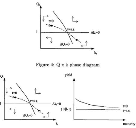
To illustrate the implications of the model, we can make use of phase

dia-grams to look at the implied dynamics and the evolution of the term structure

along time. Figure 4 shows the saddle path for the pair (Q, k). Q is above unit

for increasing k and is below unit for decreasing k.

The steady state is the point where the effective output equals the potential

one, and there is no excess demand (yt = 0). In this case, at every technology

shock that improves (worsens) eíRciency, AQ = 0 moves northeast (southwest).

The effect is similar in the case of monetary interventions that lower (rise)

the real interest rate. However, as these last interest changes are transitory, a

future.

The variety of term structure shapes and dynamics allowed makes

com-prehensive illustration unfeasible, but intuition can be gained in the analysis of

simple cases. For example, without inflation, the left diagram in Figure 5 shows

the dynamics of Q and K, and the right diagram shows the implied dynamics

of the real term structure. It is the case without intervention of an economy's

growth path.

From equation (18) it can be inferred that the real term structure becomes

flatter as the economy comes close to the steady-state (t = s.s.), since the ratios

of two different time consumptions approach unity (and the real yields approach

/3~1

for

every

maturity).

y{ is given

by:

and at t = 0 (ko below kss), the real term structure is downward sloping since

et is expected to grow at decreasing rates. The just described expansion path

contrasts the initial negative slope of the real term structure with the empirical

initial positive slope of the nominal term structure shown in section 2. This

stress our that plain RBC models, or the univariate version of Cox, Ingersoll and

Ross [24], aren't good enough to explain the nominal term structure. Something

practitioners in the financial markets are well aware of.

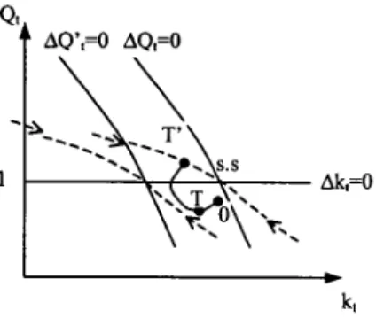
Figure 6 shows what happens when a temporary increase in the real spot

tight of the Central Bank to íight increasing inflation17: once the tight becomes

expected, Q jumps down and K begins to decrease up to the time when the

change happens (at T). Between the effective tight and the time policy is again

loosened, Q increases, while K íirst decreases, to increase after Q reaches unit.

(Q,K) changes happen so that when policy reverts to loose again (at T'), the

pair is over the original saddle and goes to the steady-state.

Figure 7, on the other hand, shows what happens when the time of the

target is uncertain. Once the change becomes justifiable by "high" inflation, Q

jumps to an intermediary saddle path, located in accordance with the proba

bility of change. While the change does not happen, inflation is increasing and

the intermediary saddle moves southwest (due to the increasing probability),

bringing together the pair (Q, K). Once the tight takes place (at T), Q jumps

again to a point that depends on the expected future monetary policy.

The combination of the real spot interest rate with the inflation dynamics

allows to obtain ali sort of shapes for the term structure.

4.6 Explanation of the stylized facts

The five stylized facts can be explained by our model.

With the spot-rate exogenously fixed, sticky inflation and adjustment costs,

the Fisher hypothesis of constant real interest rates can't hold and the expected

real spot interest rate strays from the expected marginal product of capital for

a while. A positive (negative) inflation shock not accompanied by a spot-rate

17This is an unrealistic exercise with didactical purposes only. Central Bank's interventions

jump lowers (raises) the real interest rate below (above) the present capital

productivity levei and sponsors capital investment (disinvestment). But, due

to increasing investment costs, capital does not adjust instantaneously.

Inasmuch as the expected inflation is pro-cyclical, (i) the nominal interest

rates levei is high in the peak and low in the trough of the business cycle.

Pro-cyclical nominal rates means existing bonds are expected to lose (gain)

value during the expansion (contraction) as the rates increase (decrease). The

negative of the modified duration of the bond, defined as:

O D 1

M. Duration = =

j-dy B (

shows that longer bonds are relatively more affected by the expected future

change in the levei of the term structure. Thus, (ii) the countercyclical pattern

of the term spread can be explained as a "levei upside-move risk" that is

pro-portional to the bond duration. Due to system stability, people believe there

are upper and lower bounds for the expected inflation and the probability of

a monetary authority action against inflation is increasing with inflation itself.

When the economy begins an expansion, the nominal interest rates and infla

tion leveis are low, and inflation is expected to grow. Spot rate jumps in the

near future will have positive signs, this meaning lower bond prices and capital

losses for the long maturities bond holders, who charge their borrower for that.

As expansion takes place, inflation increases, followed by the spot-rate. Since

there is a perceived upper limit for the inflation, the 'levei upside-move risk'

The description of the recession goes along the same lines.

Convexity, defined as:

d2B

1

.

Convexity = -^-0- = J {j

shows that the (iii) pro-cyclical curvature is explained by the same 'levei

upside-move risk'.

The way nominal spot interest rate is modified gives rise to a (iv) negative

short-run correlation between expected inflation and expected future real inter

est rate, since inflation innovations are not instantaneously transmitted to the

nominal spot rate.

The monetary authority operating procedure, together with inflation

sticki-ness and the system stability seem enough to justify (v) the better predictability

of the slope of the yield curve at the short- and at the long-ends respectively

(or the worse predictability of the slope of the middle of the yield curve). The

monetary authority operating procedure and inflation stickiness imply the

per-sistency of monetary policy and that inflation lasts for a while, explaining the

good predictability of the slope at the short-end of the term structure. At the

long-end, because the system is stable, long-term bond yields are mainly de

fined by the long run values, and shocks have a transitory and small impact.

Investors have reasonable certainty about inflation and the spot rate in the

near future, as well as in the long run given the system is stable. However, due

to the same inflation stickiness and operating procedures, people is uncertain

reverted, these being the causes for increased middle term uncertainty.

In the context of the present model, we have three shocks that can be

de-composed into orthogonal factors, but not interpreted as a factor itself. Our

structural shocks are not orthogonal: technology shocks may cause

expecta-tional errors and inflation, and inflation may cause spot rate jumps. Factor 1

for example, which affects ali yields with the same sign but affects long yields

less, might have considerable weight on the technology, e, and expectational

error shock, u, since both impact more short rates and die out with time. We

thus let factor interpretation for further research.

5

Model

Solution,

Simulations

and

Predictions

Equations (4), (13), (25), (26), (21) and (28) form a non-linear stochastic

differ-ence system with rational expectations that can be numerically solved according

to Novales et ai. [55] by use of Sims [63] method described in the Appendix 2.

Numerical exercises reported below used the following set of parameters:

a = 0.4 and 6 = 0.025 are standard calibration parameters for quarterly

fre-quency data. Values for cr = 2 and /? = 0.995 are in accordance with Fuhrer's

[34] similar model. A ip = 380 seems reasonable in view of the existing literature

(see Dixit & Pindyck [26]). Finally, p = 0.9 and 7 = 0.024 were estimated from

data. The procedure performed to estimate p was close to Cooley&Prescott

[20]: first assuming capital does not vary from quarter to quarter, we have

log#t - log#t_i = (logYi - logFf_i), an expression which allows building up

the

obtained

9's,

p is estimated.

The

7 was

estimated

by

instrumental

variables

using CPI inflation seasonally adjusted and the negative of the System Open

Market Accounting Holdings (per-capita and discounted a trend).

5.1 Experiments

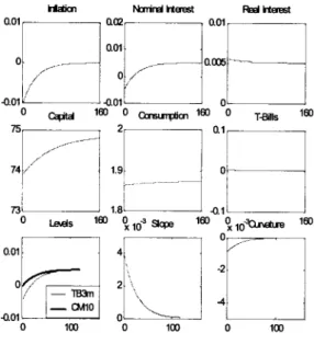
Figures 8 and 9 illustrate the dynamics of two experiments: (i) a disinflation

experiment, when infiation and capital start above the steady state (Figure 8),

and (ii) an expansion experiment, when capital as well as inflation start below

the steady state levei (Figure 9).

As shown in Figure 8, the levei of the nominal interest rates are initially

high, but the short real interest rate is expected to increase and inflation to

decrease. The evolution of the term structure is illustrated in the figure.

In Figure 9, capital and consumption increase along time, while the real

interest rates decreases.

In both cases the impulse response functions seem to describe real data18.

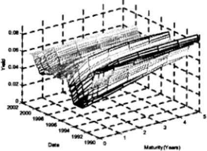
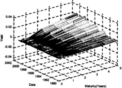
5.2 Simulation with the U.S. data

It is worth asking if the numerical predictions of the theoretical model present

patterns similar to the stylized facts in section 2.

In a attempt to test whether the model reproduces the data pattern, we have

performed the following Monte Cario exercise: given date t states 7rí_iií_2, ò?,

kt, and it+-\, to build the joint expectation conditional on the available

informa-18 More rigorous tests are certainly desirable; comparision with an unrestricted VAR seeming

tion set, 500 random paths of the modeFs variables were obtained by simulating

the system 10 years ahead, using shocks got from a bivariate normal random

00725 ]

, which is the estimated

ma-vector with covariance matrix

» -.002 .00579 ,

trix from the above residual series. With the joint expectation of the model

variables calculated, the nominal term structure on t was then defined by the

yields of the many maturity bonds:

To move from t to t + 1, and calculate the term structure on t + 1 as

just described, we assumed the realized shock to be the residual shock (et, Qt)

estimated from equations (4) and (25) from 1969:1 to 2000:4. The ? was as

the residual of the equation for estimating p. The Q was the residual of the

equation for estimating 7 (see Section 5 introduction).

The results are sensible and "close" to the qualitative pattern documented

in Section 2. Tables 4 and 5 below show the relative importance of the factors

and their respective eingenvectors.

The simulation also reproduces the correlation between expected inflation

and real interest rate. Table 6 shows the obtained values, which are close to

6

Conclusion

The simple macro model developed in this paper is able to fit the empirical term

structure of interest rates in different situations. It doesn't focus on the behavior

of some instantaneous spot rate process, derived from a particular equilibrium

model, to obtain the term structure, as usual in the literature. Instead, it

sees the spot-rate as an instrument of the monetary authority, who controls

it to match the goal of low price variation. A key behavior ai rule introduces

the needed flexibility in linking macro variables changes to movements in the

yield curve. This being the case, the long run leveis of the state variables may

be forecasted with a high degree of accuracy, as well as the future changes in

the spot rate. To obtain the term structure, people does take into account the

current drift of the inflation and what future monetary policy actions it implies.

Simulations produced results qualitatively close to several stylized facts: (i)

pro-cyclical pattern of the levei of nominal interest rates; (ii) countercyclical

pattern of the term spread (as well as low sensitivity of long yields to monetary

policy changes); (iii) pro-cyclical pattern of the curvature of the term structure;

(iv) lower predictability of the slope of the middle of the yield curve; and (v)

negative correlation of changes in real rates and expected inflation at short

horizons. Other empirical experiments may show how good is the proposed

model to fit various empirical sets of data. From a theoretical viewpoint, new

and probably more accurate, bond pricing mechanisms can be developed from

Appendices

A

The

Competitive

Problem

The equivalence of the representative consumer with a competitive economy

is shown below. As usual in the competitive framework, consumers and firms

maximize their objective function taking prices as given. Without loss of

gen-erality, it is assumed that the firms are the owners of capital and are ali equity

fmanced19.

A.1 Consumers

The consumers budget constraint is given by:

(A.l)

J=2

= (qt + dt) zt + wtk +

J=l

and the transversality conditions (6) and:

where: q is the real stock price; z is the quantity of the stocks; d is the real

dividends; wt denotes the real wage; and lt is the amount of labor.

This results in the consumers' optimal allocation rules:

For the firms decision between equity and debt in a framework similar as ours, see Brock

1 = i3Et

h+1

+^m/(ct-^)l

(A 3)

L

Qt

u'(ct)

J

and (9), (11), taking prices as given.

Given that consumers do not enjoy leisure, lt = 1 V t.

A.2 Firms

At the firm's side, the law of motion for its capital stock is:

= K?

+ If = (l-6)Kt

+ If;

where:

Kt+-\ is the capital stock to be used next period;

Kf

stands

for

used

capital

demanded

for

use

next

period;

and

if

is the

real

investment

on

new

capital.

Define the gross profits to be given by:

= f(Kulu6t)-wtlt.

Assuming firms are ali equity financed, the following identity holds:

Pvofüst = RE + dtzt,

and the ex-dividend relation is:

with RE for retained earnings and pk, t being the real price for used capital.

Financing of new and used capital obeys:

Pk, tKf + I? + <p (ç^-

- l) =RE

and the net cash flow is defined as:

- 6) pk

Nt =

+ qt (zt - zt+-\)

Thus, the firm problem can be posed as:

W (Kt) = max {Nt + Et [MUW (Kt+i)]} ,

K, l

with M-\t treated parametrically by firms20, and gives the first order conditions:

(A.4)

(A.5)

The envelope is:

= h (Kt,lt,et) - - l - S)Pkt t. (A.6)

Substituting the envelope forwarded one period into (A.4) as well as (A.4)

into (A.5) results the firnis' optimal decision rules:

Pk, t

= Et

(A.7)

^

and

taking prices as given.

It is worth pointing that by (A.3) and (32):

«Zt+1

Qt

Pfc.t

and pfc; t is equal to Tobin's marginal Q is given by:

A.3 Competitive Economy Equilibrium

An equilibrium is defined as a set of stochastic processes

ytj+V

5*'

Pk,t>

zt,

bt+-\,

k+-\,

Ct,

IA

satisfying

the

f.o.c.'s

and

the

market

clearing conditions.

Because lt = 1 V t, we can argue in terms of per capita capital kt.

To make things simpler, assume there is no issue of new shares and the firm

finances itself by retained earnings:

zt+i zt = 1,

which implies, by the ex-dividend relation and the market clearing that:

Qt = Pk,th+-\ Vi.

The economy resources constraint is thus:

(A.8)

and given the model parameters, the economy equilibrium conditions become:

Pk,t = (5Et

[í/i(A*+i

1 0t+,)-2<p('^-l)^-

+ (l-6)pkt

and

with ct given by (A.8). A system of two simultaneous equations that can be

solved for the two unknowns pk and k (or Q and k).

B

Numerical

Solution

The non-linear stochastic difference system with rational expectations (4),

(13), (25), (26), (21) and (28) can be linearized around the steady and solved

by some linear solution methods with reasonable precision, as shown in Novales

et ai. [55].

We have chosen to use Sim's [63] method to solve our model. The

proce-dure consists of dealing with each conditional expectation and the associated

expectational error as additional variables, adding to the system an equation

that defines the expectational error. In our case, we have defined the variables:

u'

and the respective expectational errors T)-\t, r]2t, r]3t.