Environment Interaction
Kai Yu1*, Sholom Wacholder1, William Wheeler2, Zhaoming Wang1,3, Neil Caporaso1, Maria Teresa Landi1, Faming Liang4
1Division of Cancer Epidemiology and Genetics, National Cancer Institute, Rockville, Maryland, United States of America,2Information Management Services, Rockville, Maryland, United States of America,3Core Genotyping Facility, SAIC Frederick, National Cancer Institute–Frederick, Frederick, Maryland, United States of America, 4Department of Statistics, Texas A&M University, College Station, Texas, United States of America
Abstract
An important follow-up step after genetic markers are found to be associated with a disease outcome is a more detailed analysis investigating how the implicated gene or chromosomal region and an established environment risk factor interact to influence the disease risk. The standard approach to this study of gene–environment interaction considers one genetic marker at a time and therefore could misrepresent and underestimate the genetic contribution to the joint effect when one or more functional loci, some of which might not be genotyped, exist in the region and interact with the environment risk factor in a complex way. We develop a more global approach based on a Bayesian model that uses a latent genetic profile variable to capture all of the genetic variation in the entire targeted region and allows the environment effect to vary across different genetic profile categories. We also propose a resampling-based test derived from the developed Bayesian model for the detection of gene–environment interaction. Using data collected in the Environment and Genetics in Lung Cancer Etiology (EAGLE) study, we apply the Bayesian model to evaluate the joint effect of smoking intensity and genetic variants in the 15q25.1 region, which contains a cluster of nicotinic acetylcholine receptor genes and has been shown to be associated with both lung cancer and smoking behavior. We find evidence for gene–environment interaction (P-value = 0.016), with the smoking effect appearing to be stronger in subjects with a genetic profile associated with a higher lung cancer risk; the conventional test of gene–environment interaction based on the single-marker approach is far from significant.
Citation:Yu K, Wacholder S, Wheeler W, Wang Z, Caporaso N, et al. (2012) A Flexible Bayesian Model for Studying Gene–Environment Interaction. PLoS Genet 8(1): e1002482. doi:10.1371/journal.pgen.1002482
Editor:Nicholas J. Schork, University of California San Diego and The Scripps Research Institute, United States of America
ReceivedJune 1, 2011;AcceptedNovember 30, 2011;PublishedJanuary 26, 2012
Funding:This work was supported by the Intramural Research Program of the National Institutes of Health, National Cancer Institute, Division of Cancer Epidemiology and Genetics. The funders had no role in study design, data collection and analysis, decision to publish, or preparation of the manuscript.
Competing Interests:The authors have declared that no competing interests exist.
* E-mail: [email protected]
Introduction
Genome-wide association studies that focus on detecting the main effect from individual single nucleotide polymorphisms (SNPs) have successfully identified more than 4,000 SNPs associated with different diseases [1]. To achieve a better understanding of the mechanisms underlying disease development, it is of great interest to follow up those genetic findings with more detailed analyses investigating how the gene and environment interact in their influence on disease risk. One popular approach aims at detecting SNP-environment interaction between individual SNPs and established environmental risk factors [2,3,4]. One of the few successes for this approach is the interaction detected between cigarette smoking and two genetic variants, a NAT2 tagging SNP and a GSTM1 deletion, in a multi-stage genome-wide association study (GWAS) of bladder cancer [3].
The standard approach to the study of gene–environment joint effect inspects one marker at a time, assuming that a single marker is the functional unit in the gene and environment interplay. This single-marker approach could misrepresent and underestimate the genetic contribution to the joint effect when one or more functional loci, some of which might not be genotyped, exist in the region, and interact with the environment risk factor in a
complex way. A more global approach that simultaneously considers all genetic markers might capture more of the genetic variation within the entire targeted region, and provides a better opportunity to reveal complicated gene–environment interactions [5]. The global approach would be more informative if it has the capability showing how an environmental effect varies according to a subject’s genetic profile.
We provide a flexible Bayesian modeling framework for the study of gene–environment joint effects. We consider a case-control study with genotypesGat a set of SNPs within a given region and a measurement for the environment exposureEavailable for each subject. We seek to identify a latent genetic profile variableLthat classifies the multilocus genotype G into different categories (clusters) such that subjects with their genotype assigned to the same genetic profile category share the same disease risk model, which is a standard logistic regression model with its own intercept term and slope. The intercept term represents the baseline log odds, common for subjects sharing the same genetic profile. The slope represents the effect (i.e., log odds ratio) of the environment risk factor for subjects with the given genetic profile. The model that we try to build and make inferences from is essentially the logistic regression model consisting ofLand Eas main effects and their product as an interaction term; the unusual aspect is that the
Copyright:ß2012 YYu et al. This is an open-access article distributed under the terms of the Creative Commons Attribution License, which permits unrestricted use, distribution, and reproduction in any medium, provided the original author and source are credited.
definition of the latent genetic profileLis a priori unknown. To account for the uncertainty in the cluster assignment underlying the definition ofL, we adopt an idea from the hidden Markov model originally developed for modeling the spatial heterogeneity of the disease event rate, observed on a predefined set of areas [6]. In this Bayesian model approach, Green and Richardson tried to allocate areas into a number of clusters and assumed a common disease rate for areas assigned to the same cluster. The mechanism for the area allocation was modeled through the Potts model [7], which favors probabilistically those allocation patterns where ‘‘neighboring’’ areas are assigned to the same cluster. Note that the spatial dependence assumption is generally appropriate in situations where the event rate is expected to take on similar values in neighboring areas. To draw the connection, we can think of each type of observed multi-locus genotypeGas an ‘‘area’’. We would like to use the Potts model to guide the cluster assignment through a certain level of ‘‘spatial’’ dependence, i.e., similar genotypes (nearby areas) tend to be assigned to the same cluster, as in other applications in genetics studies, including the study of haplotype association [8,9]. We use the Markov chain Monte Carlo (MCMC) sampling method (e.g., [10,11]) to fit the proposed model, incorporating several recent advances in the MCMC methodology. We adopt a recently developed algorithm [12] to update the regulating parameter in the Potts model, which has an intractable normalizing constant, and cannot be handled by the standard Metropolis Hastings algorithm. This algorithm allows us to consider the parameter of interest on its original continuous scale and obviates the need for a finite number of selected grids with their normalizing constants pre-calculated, a strategy taken by Green and Richardson [6]. To identify the optimal genetic profile assignment, we use an ensemble averaging method that aggregates different cluster assignments generated by the MCMC samplers into a consensual one. We find that this cluster algorithm works quite well in simulation studies. A similar idea has been used by Liang [13] and Molitor et al[14] in different contexts. We also propose a resampling-based test based on the fitted Bayesian model that can be used to formally test for the existence of gene– environment interaction.
We apply the proposed method to study the joint effect of cigarette smoking intensity and genetic variants in chromosome
region 15q25.1 using data from EAGLE, a population-based case-control study conducted in Italy [15]. Cigarette smoking is an established major risk factor for lung cancer. Besides environmen-tal exposures, recent GWAS identified a few chromosome regions (e.g., chromosomes 15q25.1, 5p15, and 6p21) harboring genetic variants underlying a susceptibility for lung cancer [15,16,17]. In particular, the chromosome 15q25.1 region, which includes the CHRNA5-CHRNA3-CHRNB4 cluster of cholinergic nicotinic receptor subunit genes, has been shown to be associated with both lung cancer and smoking behaviors, such as cigarette smoking intensity [18,19,20,21,22]. Although there is no evidence suggest-ing the existence of multiple loci in this region independently contributing to lung cancer susceptibility in populations of European ancestry [16], it does appear that there are multiple independent loci within 15q25.1 affecting smoking intensity [19]. The main goal of our analysis is to evaluate whether the effect of smoking intensity varies with genetic variants in 15q25.1. Our analysis finds evidence for gene–environment interaction, with the relative risk for smoking appearing to be stronger in subjects with a genetic profile associated with a higher lung cancer risk. The proposed resampling-based test derived from the fitted Bayesian model also detects significant gene–environment interaction (P-value = 0.016). On the other hand, the standard single-marker approach that aims at detecting the interaction between a SNP and smoking intensity fails to reveal any evidence of interaction, with the smallest observed nominal P-value being 0.021 among the 32 testing SNPs, and the adjusted P-value based on the permu-tation test being 0.29.
Materials and Methods
We first introduce the Bayesian model and describe the MCMC algorithm for fitting this model. Next we provide procedures for posterior inference using samples generated by the MCMC sampler, including a method for deciding the number of clusters and a method for identifying the optimal cluster assignment once the number of clusters is determined. We validate the proposed method using simulated data. We then apply the method to study the gene–environment joint effect using data generated from the EAGLE lung cancer case-control study.
The Bayesian Model Setup
Assume we have data collected from a case-control study, with n1 cases, n0 controls. Let n~n0zn1 be the total number of subjects in the study. For the ith subject, we denote its observation by ðYi,Ei,Xi,GiÞ, where Yi~1 for a case, 0 for a control; Ei is the observed exposure for the environment risk factor of interest;Xi represents measures on a set of covariates; andGirepresents multilocus genotypes observed on a set of SNPs in a pre-specified region. In the following discussion, we use the term genotype to refer to the multilocus genotype observed on all considered SNPs within the targeted region. We intend to develop a model for the G-E joint effect that permits G-E
interaction. More specifically, we assume the true underlying risk model has the following form:
log p(Yi~1) 1{p(Yi~1)
~
a1zb1Eizt’Xi, ifGi[cluster 1,
a2zb2Eizt’Xi, ifGi[cluster 2,
:::
aKzbKEizt’Xi, ifGi[clusterK,
8 > > > <
> > > :
ð1Þ
where clusters 1 toKrepresent a partition of the genotype space; ak is the intercept term representing the common baseline log Author Summary
odds for subjects with their genotypes in clusterk;bkis the effect ofE(in term of log odds ratio) in the disease model for clusterk, k~1,:::,K; and t is the vector of coefficients for the set of covariates X and is constant regardless of a subject’s genotype. Notice that if the partition of the joint genotype space is known a priori, we can derive the correspondingK-category genetic profile variableLbased on the cluster assignment. The above model (1) is then essentially the standard logistic regression model consisting of LandE as main effects and their product as the interaction term, with adjustment forX, and has the following form:
log Pr (Yi~1) 1{Pr (Yi~1)
~a1zt’Xizb1Eiz XK
k~2 ak{a1
ð ÞI(Li~k)z
XK
k~2 bk{b1
ð ÞEi|I(Li~k):
Thus it is clear that there is noG-E interaction ifb1~b2~ ~bK, and the interaction exists if otherwise.
In real applications, we do not know a priori the partition of the genotype space. IfG consists of just one SNP, the goal can be achieved easily by using a saturated logistic regression including bothE andG(as a three-level categorical variable) as the main effects and their product as the interaction term. For situations whereGconsists of multiple SNPs (e.g., more than 10), as in the case of the EAGLE lung cancer study, we propose the following Bayesian model that simultaneously searches for the optimal partition of the genotype space and estimates the unknown parameters in the corresponding risk model (1).
The Bayesian model is built up in a hierarchic framework. We first describe our model by assumingK, the total number of clusters, is known. We will describe how to chooseKlater. Suppose there are
Htypes of genotype configurations observed in the sample, labeled as genotype 1, 2, …,H. We define the latent genotype allocation vectorz~(z1,:::,zH), withzh[f1,:::,Kg, being the cluster
assign-ment for genotype h, h~1,:::,H. For subject i, we denote its genotype id byhi. Given the allocation vectorz~(z1,:::,zH)and the set of coefficientsC~f(ak,bk,t),k~1,:::,Kgfor the disease model (1), the probability of subjectihaving the disease outcome is
p(Yi~1jz,C)~
exp (azh
izbzhiEizt
’Xi)
1zexp (azh
izbzhiEizt
’Xi),i~1,:::,n: ð2Þ
In the above model specification, we use the prospective likelihood function (2) for observed case-control data, which were collected under a retrospective sampling scheme given the disease outcome. The use of the prospective likelihood function can be partially justified by the general results from Staicu [23] and Seaman and Richardson [24]. They showed the equivalence of prospective and retrospective analysis in the Bayesian framework in the sense that both approaches could yield the identical marginal posterior distribution of the log odds ratio under analyses with properly specified priors. In model (2), the effect of
Evaries withG. Thus we call it the Bayesian risk model allowing for G-E interaction. As a comparison in the analysis, we also consider a model assuming a homogeneous effect fromE, which is defined as
p(Yi~1jz,C)~
exp (azh
izbEizt
’Xi)
1zexp (azh
izbEizt
’Xi)
,i~1,:::,n: ð3Þ
We call this model the Bayesian risk model without G-E
interaction. In what follows, we will describe methods for fitting model (2), the one allowing for G-E interaction. Similar procedures can be applied to model (3).
To model the distribution of the allocation vector z, we first choose a similarity metric to define the spatial contiguity between any two genotypes. LetJdenote the total number of considered SNPs within the region, with the genotype at a given SNP being coded as 0, 1, or 2 according to the number of copies of the minor allele. Let genotypes h and h’ have the configurations
gh,1,:::,gh,J
ð Þ and ðgh’,1,:::,gh’,JÞ, wheregh,j is the genotype at the jth SNP for the multilocus genotype h. We first define the distance between them as
dh,h’~
ffiffiffiffiffiffiffiffiffiffiffiffiffiffiffiffiffiffiffiffiffiffiffiffiffiffiffiffiffiffiffiffiffiffiffiffi 1
J XJ
j~1
gh,j{gh’,j
2 v2 j v u u t ,
wherev2 j~
Pn i~1
ghi,j{ggj
2
n{1 is the variance for the genotype at SNP
jobserved in the sample, withghi,jbeing the genotype at SNPjfor
subject i, and ggj~ 1 n
Xn
i~1
ghi,j. Then we define sh,h’~1 if h’ is
among the 4 (distinctive) genotypes closest to genotypeh, andhis among the 4 genotypes closest to genotypeh’;sh,h’~0:5ifh’(orh)
is among the 4 genotypes closest to genotypeh(orh’) but this is not true in both cases; andsh,h’~0for all other cases.
We model z with the Potts model, which has a regulating parameter y governing the level of spatial dependency in the cluster assignment. The Potts model has the following form:
pK(zjy)~exp½yU(z){hK(y),
where U(z)~ P h=h0
sh,h0I½zh~zh0, with I½zh~zh0 being the
indictor function, i.e., I½zh~zh0~1if zh~zh0 and 0 otherwise, and where
hK(y)~log
X
z[f1,2,:::,KgH
exp½yU(z)
0
@
1
A
is the log normalizing constant. Under the Potts model withy~0, the cluster assignments are allocated independently for different genotypes. Whenyw0, the cluster assignments for two neighboring genotypeshandh’(i.e., two genotypes withsh,h’w0) are correlated.
The level of correlation (spatial dependence) increases withy. For example, under the genotype configuration observed in the EAGLE study andK~2, the average probability that any two neighboring genotypes are allocated to the same cluster is 0.5 wheny~0:0. It increases to 0.83, and 0.97 fory~0:6and 1.2, respectively. More discussions of the Potts model can be found in [6].
interval ½0,ymax, which covers an appropriate region ofy such that the resulting class of Potts models are flexible enough to capture a wide range of spatial dependence. We note thatymaxcannot be too large. Ifyis over a critical point, the corresponding Potts model would essentially force almost all elements into the same cluster, a well known phenomenon for the Potts model called phase transition property [25], and in this situation, the MCMC simulation tends to get stuck. We did some experiments to explore the setting ofymax for the Potts model based on the neighborhood configuration observed in the EAGLE study. We found the valuey~1:2induces a high level of spatial dependence, with the average probability that any two neighboring genotypes are allocated to the same cluster being 0.97 atK~2; and wheny~1:5, the average probability goes to 0.99, which indicates an extremely high level of spatial dependence for the Potts model. Based on these observations, we decided to setymax~1:2in our EAGLE study application, as well as in simulation studies that assume the same neighborhood structure as the EAGLE study. We consider only a uniform prior for ysince in practice we usually do not know which level of spatial dependence is more likely than the others. But the algorithm described below can certainly be used with other prior functions if necessary.
Putting all the foregoing models together, we can express the joint distribution of all variables as
p(y,C,zjY)!p(y)p(C)p(zjy)p(YjC,z),
where p(YjC,z)~ Pn i~1p(YijC,
z). The inference (for a fixed total number of clustersK) ony,C, andzcan be based on the following MCMC algorithm.
The MCMC Algorithm
Updating coefficients C. The full conditional function for coefficients C~f(ak,bk,t),k~1,:::,Kg in the risk model can be written as
p(Cj )!p(C)|P n
i~1
I(Yi~1) exp (azh i
zbzh iEi
zt’Xi)
1zexp (a
zhizbzhiEizt’Xi) z 2
4
I(Yi~0) 1zexp (azh
izbzhiEi zt’Xi)
3
5:
ð4Þ
We can use the standard Metropolis-Hastings (MH) steps to updateC, conditioned on the current values of other parameters. The detailed algorithm is given in Text S1.
Updating the allocation vector z. Following Green and
Richardson [6], we can update the allocations zusing a Gibbs kernel; that is, for the genotypeh, its cluster assignment is updated by drawing from the following full conditional distribution,
p(zh~kj )!exp ytkhð Þz
|P i:hi~h
I(Yi~1) exp (akzbkEizt’Xi) 1zexp (akzbkEizt’Xi)
z I(Yi~0) 1zexp (akzbkEizt’Xi)
,
k~1,:::,K, ð5Þ
where tk hð Þz~
P
h’:zh’~k,h0=h
sh,h0 is the sum of similarity scores
between the genotypehand other genotypes currently assigned to clusterk.
Since the sampling space forzis discrete, the standard Gibbs sampler can be improved by the Metropolized Gibbs sampler [26]. Thus we choose this sampler for updating the allocation vector. A summary of the algorithm is given in Text S1.
Updating the regulating parameter y. The regulating parameteryhas the following full conditional distribution:
p(yj )!p(y) exp½yU(z){hK(y): ð6Þ
If the standard MH algorithm is used, updatingywould involve the evaluation of the normalizing constant hK(y) for the Potts model, which is prohibitive when the dimension of z is large. Green and Richardson [6] chose to restrictyto a pre-specified finite set of values; they used the thermodynamic integration approach [27] to estimatehK(y) for a given value of K. Those estimates were then used in the MCMC sampler. The estimate of hK(y) at pre-specified grid points might lead to biased Monte Carlo estimates ofyand other parameters.
Here we propose to use the recently developed Monte Carlo Metropolis-Hastings algorithm (MCMH) [12] to sampleyfrom p(yj ). This new algorithm replaces the ratio of normalizing constants at any two values of y by a Monte Carlo estimate, which is obtained through a set of mauxiliary samples, in the MCMC iterations, thus allowing us to consideryon its original continuous scale instead of on a finite number of pre-specified points. As shown in [12], this algorithm ensures that the Monte Carlo estimate of the parameter will converge to its posterior mean. In our numeric experiments, we find it is appropriate to choose the number of auxiliary samplesmto be between 50 and 100. A summary of the algorithm for updatingyis given in Text S1.
Posterior Inference
In our simulation studies and the real data application, we find the MCMC algorithm generally converges after 100.000 iterations. Below we describe a procedure for determining the number of clusters, and an ensemble averaging method for the identification of the cluster assignment based on the MCMC samples.
Determining the number of clusters. We choose to use the deviance information criterion (DIC) proposed by Spiegelhalter
et al [28] for determining the number of clusters. For a given number of clustersK, define the devianceDK(Y,C,z)as
DK(Y,C,z)~{2 lnP n
i~1p(YijC, z):
We can calculate the posterior expected devianceE D½ K(Y,C,z)jY by averaging the deviance calculated at samples of(C,z)generated by MCMC output. We calculate the devianceDK(Y,CC,zz)at the posterior mean of the parameters as
DK(Y,CC,zz)~{2 lnP n
i~1
I(Yi~1) exp (aa(i)zbb(i)Eiztt’Xi) 1zexp (aa(i)zbb(i)E
iztt’Xi) z "
I(Yi~0) 1zexp (aa(i)zbb(i)E
iztt’Xi)
,
where aa(i) and bb(i)
DICK~2E D½ K(Y,C,z)jY{DK(Y,CC,zz):
To determine the number of clusters, we run the algorithm with different values of K (e.g., K~1,:::,Kmax, with Kmax~8) and compute their DIC values. The DIC criterion favors models with small DIC values. To take the Monte Carlo variation into the consideration, instead of choosing theKwith the smallest DIC, we adopt the+1 standard error (SE) rule originally proposed for the tree model selection [29]. To use this rule, we run the MCMC algorithm 20 times, with different random seeds for each considered value of K, and then pick the optimal number of clustersKas the smallest one such that
ave(DICK)vave(DICK0)zse(DICK0), ð7Þ
whereave(DICK)is the average of the values of DIC measured at K over 20 runs, K0~arg min1ƒKƒKmaxave(DICK), and
se(DICK0) is the Monte Carlo standard error estimated for
DICK0 based on 20 runs.
Based on our numerical experiments, we found that the Monte Carlo standard error usually is less than 1 if the MCMC chain converges. So, if there is only one run for eachK, we recommend pickingKas the smallest one such that
DICKvmin1ƒKƒKmaxDICKz1: ð8Þ
We use this rule, hereafter called the+1 rule, to select the optimal number of clusters in simulation studies.
Identifying the cluster assignment. After the determi-nation of the number of clustersK, it is usually helpful to identify the consensual cluster assignment rule that assigns each genotype to one of theKclusters. We can also use this partition to assign each subject to one of the clusters based on his or her genotype’s assignment. Here we adopt the ideas from Liang [13] and Molitor
et al[14] to find such a partition. Based on the samples generated from MCMC runs under theK-clustermodel, we letc
h,h’be the
proportion of times that the genotypeshandh’are assigned to the
same cluster. We then use ffiffiffiffiffiffiffiffiffiffiffiffiffiffiffi1{ch,h’
p
as the dissimilarity metric and apply the PAM (partitioning around medoids) method [30] to partition genotypes intoKclusters. Simulation studies presented later show this clustering algorithm works quite well in identifying the appropriate clusters.
A Resampling-Based Test for Gene–Environment Interaction
It is usually desirable to have a formal statistical test or decision rule for inference regarding the presence of an interaction. Here we propose a resampling-based test for this purpose. First we fit model (2), the Bayesian risk model allowing forG-Einteraction, under various numbers of clusters. Then we use the +1 rule to identifyK, the optimal number of clusters that is not less than 2, and the corresponding consensual cluster assignment L. We requireK§2for this interaction test because the interaction test is not defined forK~1. We use the maximum likelihood estimate (MLE) to establish the following logistic regression model,
log Pr (Yi~1) 1{Pr (Yi~1)
~c1zl’Xizm1Eiz
XK
k~2
ckI(Li~k)z XK
k~2
mkEiI(Li~k), ð9Þ
whereLiis the cluster assignment for subjecti,i~1,:::n, given by the consensual cluster assignmentL. This model includes the main effects ofLandE, as well as their interactions. We can conduct a likelihood ratio test comparing model (9) with the similar model without the interaction terms and obtain the corresponding ‘‘P-value’’, denoted byd, based on the Chi-squared distribution with K{1degrees of freedom (df). Clearly, this ‘‘P-value’’dtends to overestimate the significance level of the interaction, as the variableLis data-driven, but a small value fordprovides evidence against the null. We can usedas the test statistic and apply the following resampling-based procedure to evaluate its significance level.
1. Apply the MCMC procedure to fit model (3), the Bayesian risk model without G-E interaction, on the observed data and identify KNull §2, the optimal number of clusters, using the +1 rule, as well as the corresponding consensual cluster assignment.
2. Use MLE to fit the following logistic regression model based on the observed data,
log Pr (Yi~1) 1{Pr (Yi~1)
~ X KNull
k~1 ~
cckI(LNulli ~k)z~ll’Xizmm~Ei,ð10Þ
whereLNull
i is the cluster assignment for subject i,i~1,:::n, given by the consensual cluster assignment identified in Step 1, and~mm,~cck,k~1,:::,K
Null, and^llare the estimated coefficients. 3. Use the model given by (10) to generateBsets of bootstrap null datasets. Each null dataset is a copy of the observed dataset, except the outcome for every subject is regenerated according to the probability model given by (10).
4. For thebth null dataset,b~1,:::,B, obtain the test statisticd(b) using the same procedure used above for obtainingd.
5. The estimated P-value fordis given by 1 B
XB
b~1
I(d(b)vd)
In Steps 1 and 2 we establish the Bayesian risk model under the null hypothesis that there is no G-E interaction and the corresponding logistic regression model. We use the fitted logistic regression model (10) to generate multiple null datasets in Step 3 based on the parametric bootstrap procedure [31]. In Step 4, for the bth generated null dataset, we first apply the MCMC procedure to establish the Bayesian model given by (2) and next identify the optimal number of clusters with the+1 rule, as well as the corresponding consensual cluster assignment. Then we fit the corresponding logistic regression model withG-Einteraction and obtain the test statisticd(b) from the likelihood ratio test.
Results
The EAGLE Study
represent each subject’s genetic variation pattern in the region. The reason for removing redundant SNPs is to ensure that the similarity measure between any two types of multilocus genotypes is not dominated by a set of SNPs in high linkage disequilibrium. The summary of the 15 chosen tagging SNPs is given in Table 1.
Simulation Studies: Performance of the Bayesian Model
We conducted simulation studies to evaluate the performance of the proposed method for fitting the Bayesian model allowing for
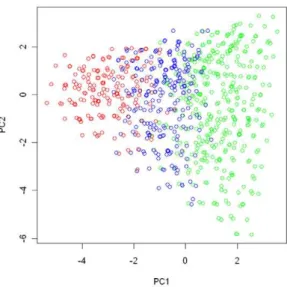
G-E interaction. In the simulation study we were interested in studying the interaction between a binary environment risk factor (E~0or 1) and genetic variants (G) within a candidate region. We used genotypes at 15 tagging SNPs (Table 1) in 15q25.1 observed in the EAGLE study to represent the joint genotype distribution for the simulated population, which consisted of 766 distinct multilocus genotypes. We chose the 2nd, 6th, and 10thSNPs listed in the Table 1 as the functional SNPs, and divided the genotype space into the following three regions according to the total number of risk alleles (assuming the minor allele to be the high-risk allele) among the 3 functional SNPs: region I, consisting of genotypes with g2zg6zg10ƒ1; regions II, consisting of geno-types withg2zg6zg10~2; and region III, including genotypes withg2zg6zg10w2. We conducted a principal component (PC) analysis on subjects from the EAGLE study with genotypes at the 15 SNPs as their coordinates. Figure 1 shows how genotypes (subjects) in each of the three regions were distributed in the first 2-PC space, with regions I, II, and III in green, blue, and red, respectively.
The disease risk models we considered had the form given by (1). Their definitions are given in Table 2. Under ModelM1there was no genetic effect and no interaction betweenGand E, and thus there was no risk heterogeneity in the genotype space. Under M2andM3, coefficientsaandbhad the same clustering pattern. Under modelsM4, the risk heterogeneity patterns foraandbwere not matched, unlike those under modelM2andM3. In modelM4, the two clusters defined byawere region I, and regions II and III combined, while the two clusters defined by the effect ofb were regions I and II combined, and region III.
We assumed that the environmental exposure statusE(0 or 1) andGwere correlated in the general population. The distribution of E depended on G in the following way: for a subject with genotype in region I, the probabilities of being unexposed (E~0) or exposed (E~1) were 0.7 and 0.3; for a subject with genotype in one of the other two regions, those probabilities were 0.4 and 0.6 forE~0andE~1. Thus the distribution ofEwas quite different for subjects with different genotypes.
Under each model, we simulated 50 datasets representing a case-control study with 1500 cases and 1500 controls. We ran the MCMC algorithm with 2,000,000 iterations with the first 1,000,000 iterations being discarded. We used an algorithm similar to that described in [32] to simulate the case-control study. Note that under the case-control sampling scheme, we do not need to specify a value fora1. Instead, we just need to know the values ofai{a1,i~2,3, in order to simulate datasets from a case-control study.
For each simulated dataset, we applied our method withm~50 auxiliary samples, with the number of clustersKranging from 1 to 8. We used the+1 rule defined by (8) to identifyK, the optimal number of clusters. Table 3 provides a summary of the number of clusters identified over 50 simulated datasets under each risk model. We can see from the table that the+1 rule performs quite
Table 1.Summary of 15 tagging SNPs chosen for the EAGLE study.
SNP id Position MAFa Oddsratiob P-valueb PC1c PC2c
rs1394371 76511524 0.32 1.110685 7.34E-02 0.238102 0.289431
rs12903150 76511700 0.22 0.916667 1.89E-01 20.22088 0.066403
rs12899131 76513940 0.38 0.973222 6.27E-01 20.36255 0.013854
rs2656069 76532762 0.23 0.760253 7.67E-05 0.110054 20.40066
rs13180 76576543 0.39 0.873685 1.75E-02 20.08845 20.374
rs3743079 76578116 0.17 1.075484 3.13E-01 20.2273 20.05414
rs3885951 76612972 0.12 1.279568 2.30E-03 0.158959 0.186958
rs2036534 76614003 0.24 0.698668 1.23E-07 0.120671 20.42301
rs2292117 76621744 0.36 0.908155 8.78E-02 20.39076 0.034655
rs680244 76658343 0.37 0.911216 1.03E-01 20.39566 0.037326
rs578776 76675455 0.29 0.738028 1.45E-06 0.085806 20.39304
rs12914385 76685778 0.41 1.416705 3.68E-10 0.258519 0.31863
rs1948 76704454 0.3 0.878962 3.10E-02 20.36327 0.013799
rs11636753 76716001 0.35 0.89959 6.74E-02 20.35628 0.025404
rs12441998 76716427 0.24 0.725298 2.24E-06 0.096535 20.36738
aThe minor allele frequency was estimated based on the control samples in the
EAGLE study.
bThe per-allele OR and the one degree of freedom Wald test for the association between lung cancer and the SNP based on the logistic regression model adjusted for smoking intensity, age, and gender. The SNP genotype was coded as the copy number of the minor alleles.
cLoadings of individual SNPs on the first and second principal components
based on the principal component analysis conducted on the selected subjects from the EAGLE study used in the real-data application. The highlighted values in the PC2 column are the ones that dominate the definition of the 2nd principal component.
doi:10.1371/journal.pgen.1002482.t001
Figure 1. The partition of the genotype space in the simulation study.We conducted a principal component analysis on all subjects from the EAGLE study with genotypes at the 15 chosen tagging SNPs as coordinates. We plot subjects by their first and second principal components. Subjects with the same multilocus genotype were represented by a single point in the plot. The points in green, blue, and red colors are those subjects (genotypes) belonging to region I (consisting of genotypes having no more than 1 risk allele among the three considered functional SNPs), region II (consisting of genotypes having 2 risk alleles), and region III (consisting of genotypes have more than 2 risk alleles).
well in identifying the right number of clusters, even in situations where there is no clustering structure (i.e., the true number of clusters,Ktrue, is 1).
We evaluated the performance of the algorithm for cluster assignment by comparing the cluster assignment estimated at K~Ktrue with the true underlying cluster assignment chosen by the simulation design. For modelM4, the clustering patterns fora and b were not matched. In this case we treated the finer partitioning (given by Figure 1) that accommodates the clustering patterns of both a and b as the true one. The accuracy of the estimated cluster assignment was measured as the proportion of subjects being assigned to the same cluster by both assignments (the estimated one and the true one). The accuracy summary over 50 replications under various considered models (exceptM1, the model with no clustering structure) is given in Table 4. It indicates that the cluster assignment algorithm appears to be able to partition the subjects (and genotypes) into the proper subgroups, provided that the correct number of clusters can be identified.
We also evaluated the accuracy of the estimated coefficients (a andb). Based on the true risk model (1), subjectiwith genotypehi was assigned to one of the risk models. We considered coefficients aandbin that risk model to be the true coefficient values for this subject. Thus, subjects with their genotypes belonging to the same cluster would share the same true coefficient values. We usedbb^(i), the posterior median ofbassigned to subjectibased on MCMC samples generated under K~K, as the estimates for the underlying coefficients. The number of clustersKwas estimated by the +1 rule, as described previously. Since the odds for the genetic effect is not identifiable under the case-control design, we were interested only in the difference inabetween two groups. To
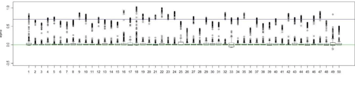
present the result for each experiment, we shifted the value of^aa(i), the posterior median ofafor subjecti, by a constant value, which was chosen asmedianj[Clusterkaa^(j), the median of^aaamong subjects in true cluster 1. As a result, the median level of the shifted pos-terior median (we still represent it as^aa(i)) among subjects in cluster 1 is 0. In Figure 2, Figure 3, Figure 4, and Figure 5, we present summaries of^aa(i) and ^bb(i)
for each of the 50 experiments under modelsM2andM3. Summarized results for modelM4are given in Figures S1 and S2. Each boxplot is a summary of^aa(i) orbb^(i) among subjects in a true underlying cluster. From those figures, we can see that the estimates align with their true values quite well. Notice that these estimates were obtained under the model with the number of clusters estimated by the+1 rule.
We inspected the algorithm’s convergence using the Gelman and Rubin’s diagnostic plot [33], as implemented in the CODA R package [34]. For each model, we checked the convergence on the first 5 simulated datasets used in the above simulation studies, with 5 independent runs on each dataset. We found that the proposed algorithm can converge within 100,000 iterations, with the estimated shrinkage factor falling below the recommended threshold of 1.1. We also show in Figures S3 and S4 the posterior distributions forbk,k~1,2,3, resulting from each of 5 indepen-dent runs on the first simulated dataset under modelsM3, andM4. It is evident from these plots that we can obtain very consistent posterior distributions for parameters of interest among different runs on the same data.
Simulation Studies: Performance of the Resampling-Based Test
We conducted a simulation study to evaluate whether the proposed resampling-based test can maintain the proper type I
Table 2.List of disease risk models considered in the simulation study for evaluating the Bayesian model.
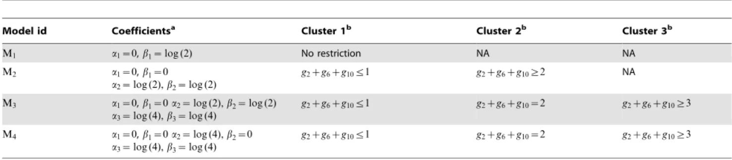
Model id Coefficientsa Cluster 1b Cluster 2b Cluster 3b
M1 a1~0,b1~log (2) No restriction NA NA
M2 a1~0,b1~0
a2~log (2),b2~log (2)
g2zg6zg10ƒ1 g2zg6zg10§2 NA
M3 a1~0,b1~0a2~log (2),b2~log (2)
a3~log (4),b3~log (4)
g2zg6zg10ƒ1 g2zg6zg10~2 g2zg6zg10§3
M4 a1~0,b1~0a2~log (4),b2~0
a3~log (4),b3~log (4)
g2zg6zg10ƒ1 g2zg6zg10~2 g2zg6zg10§3
aThe coefficients are defined for models with the form given by (1) in the main text.
bThe cluster is defined according to the total number of risk alleles at the three chosen SNPs (the 2nd, 6th, and 10thSNPs listed in Table 1).
doi:10.1371/journal.pgen.1002482.t002
Table 3.Performance of the+1 rule for identifying the number of clusters in the simulation study.
Total number of clusters identified (K)
Model id K~1 K~2 K~3 K~4 K§5
M1 48 1 1
M2 46 3 1
M3 45 5
M4 42 7 1
There are 50 simulated datasets under each model. The counts are the frequencies for the number of clusters identified by the+1 rule defined in the main text. The highlighted counts are the number of times the algorithm identified the correct number of clusters.
doi:10.1371/journal.pgen.1002482.t003
Table 4.Performance of the algorithm for the cluster assignment.
Accuracy Summary
Model id Mean
Standard Deviation
M2 0.95 0.011
M3 0.92 0.019
M4 0.93 0.017
The accuracy summary for the cluster assignment is based on 50 simulated datasets under each model. The cluster assignment is estimated under the correct number of clusters.
error rate. We considered a disease risk model that had the main effects fromG(with OR = 4 for genotypes falling into regions II and III vs. those in region I) andE(with a common OR of 4 for E~1vs.E~0), with no interaction betweenGandE. Regions
are defined in Figure 1. We assumed a study sample size of 600 cases and 600 controls, and simulated 1000 datasets under the considered risk model as did before. For each dataset, we ran the resampling-based test with 1000 bootstrap steps for the estimation
Figure 2. Boxplots of the posterior medians of the intercept (a) for subjects within each true cluster from each of 50 datasets simulated under the modelM2.(a). Boxplots of posterior medians ofafor subjects in cluster 1, with the true value given by the horizontal line in
green; (b). Boxplots of posterior medians ofafor subjects in cluster 2, with the true value given by the horizontal line in blue. The posterior median of
afor each subject under a given simulated dataset was shifted by a constant value selected so that the median value of the shifted estimates for subjects in cluster 1 was zero.
doi:10.1371/journal.pgen.1002482.g002
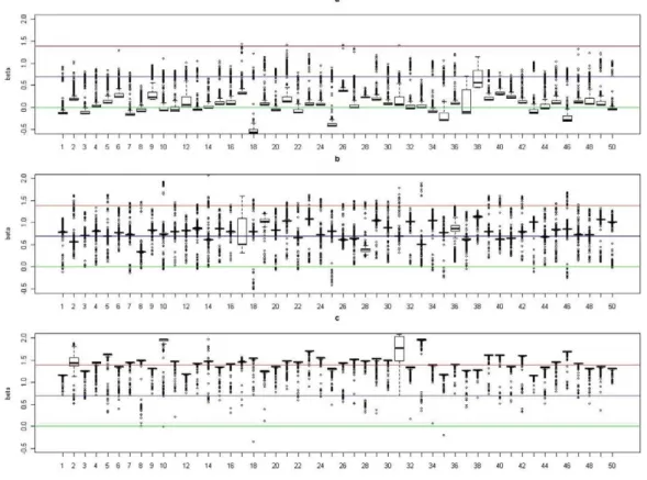
Figure 3. Boxplots of the posterior medians of the log odds ratio (b) for subjects within each true cluster from each of 50 datasets simulated under the modelM2.(a). Boxplots of posterior medians ofbfor subjects in cluster 1, with the true value given by the horizontal line in green; (b). Boxplots of posterior medians ofbfor subjects in cluster 2, with the true value given by the horizontal line in blue.
of the P-value, allowing the number of clusters to vary from 2 to 5. To reduce the computing time further, we ran the MCMC algorithm for 300,000 iterations with the burn-in period consisting of the first 200,000 iterations for each bootstrapped sample (as 200,000 iterations appear to be enough to ensure the convergence of the MCMC algorithm). We found that the proposed resampling-based test can maintain the proper type I error in the considered scenario, with estimated false positive rates of 0.055 and 0.097 under nominal levels of 0.05 and 0.10, respectively.
We compared the power of the proposed resampling-based test with two other standard interaction tests, the minP-SNP and minPC tests. Both test statistics are based on the minimum P-value observed on a set of univariate G-E interaction tests, with their significant levels being evaluated through a resampling-based procedure. The minP-SNP test is based on the set of single SNP-environment interaction tests, with each SNP-SNP-environment interaction test statistic being derived from the standard likelihood ratio test comparing two logistic regression models with and without the SNP-environment interaction term. The SNP effect is modeled with a categorical variable with three levels so each SNP-environment interaction test considered in the minP-SNP test is a 2 df test. The minP-PC is based on a set of tests that evaluate the interaction between a single principal component (PC) and the environment variable. PCs are derived from the principal component analysis of genotypes on all considered SNPs. Similar to the minP-SNP test, each PC-environment interaction test is derived from the likelihood ratio test comparing two logistic regression models with and without the interaction term. The PC effect is model as a continuous variable. Both minP-SNP and
minP-PC were based on 15 univariate tests in the simulation study as there were a total of 15 SNPs in the considered chromosome region.
We evaluated the power under six different disease risk models, including M2, M3, and M4 defined in Table 2, and the three additional models MSNP1, MSNP2, andMEAGLE. Model MSNP1 andMSNP2had just one functional SNP (the 10thSNP in Table 1). ModelMSNP1 had 2 clusters, with coefficients in the formula (1) being a1~b1~0 for genotypes satisfying the condition g10~0 (cluster 1), anda2~b2~log (4)forg10~1, or 2 (cluster 2). Model MSNP2 had 3 clusters, with coefficients a1~b1~0 for g10~0 (cluster 1), a2~b2~log (2) for g10~1 (cluster 2), and a3~b3~log (4)for g10~2(cluster 3). ModelMEAGLE adopted a 2-cluster pattern observed in the analysis of the EAGLE study described later, with clusters 1 and 2 consisting of genotypes in red and blue colors, respectively (Figure 6), and witha1~b1~0for cluster 1, and a2~b2~log (4) for cluster 2. The correlation betweenEand Gwas defined similarly as before. For a subject with genotype in cluster 1, the probabilities of being unexposed (E~0) or exposed (E~1) were 0.7 and 0.3; for a subject with genotype not in cluster 1, those probabilities were 0.4 and 0.6.
environment interaction test based on the 10th SNP is most optimal, due to the multiple comparison adjustment, the minP-SNP test is only slightly more powerful than the proposed test. Under the modelMSNP1where the functional SNP (the 10thSNP)
has a dominant effect in its interaction withE, the minP-SNP test compares less favorably with the proposed test since each of single SNP-environment interaction test considered in the minP-SNP global test spends one more df than necessary (as there are only two cluster in the modelMSNP1). The minP-PC test has the worst overall performance as it is very sensitive to its underlying assumption that the genetic effect is linearly correlated with one of the PC direction.
Application in the EAGLE Study
We applied the proposed method to study the joint effect of cigarette smoking intensity (number of packs per day) and genetic variants in chromosome region 15q25.1 on lung cancer risk, using data generated by the EAGLE study. We focused on former and current smokers who had been genotyped on the 15 tagging SNPs. We also removed, as outliers, 8 subjects who had smoked more than 3 packs of cigarette per day. The final dataset for our analysis consisted of 1326 controls and 1720 cases. In the analysis we treated smoking intensity as a continuous variable and adjusted for the effects of gender and of age at diagnosis (categorized as: ,= 60, 61–70,.70). We used a Bayesian model that allowed for
G-Einteraction, unless specified otherwise.
To determine the number of clusters, we ran the MCMC algorithm 20 times with different random seeds for each K, K~1,:::,8, in order to estimate the Monte Carlo standard error for DIC. Figure 7 shows the DIC values for each K over 20 replications. Based on the 1 SE rule given by (7), the optimal number of clusters was found to be 2, with its averaged DIC value being 3810.5. The partitioning of subjects into 2 clusters based on our proposed clustering algorithm is very consistent among 20
Figure 5. Boxplots of the posterior medians of the log odds ratio (b) for subjects within each true cluster from each of 50 datasets simulated under the modelM3.(a). Boxplots of posterior medians ofbfor subjects in cluster 1, with the true value given by the horizontal line in green; (b). Boxplots of posterior medians ofbfor subjects in cluster 2, with the true value given by the horizontal line in blue; (c). Boxplots of posterior medians ofbfor subjects in cluster 3, with the true value given by the horizontal line in red.
doi:10.1371/journal.pgen.1002482.g005
Figure 6. Cluster assignment for the EAGLE study.The cluster assignment estimated under the model with the number of clusters K= 2. Every subject was represented by his or her first 2 principal components. Subjects with the same multilocus genotype were represented by one point in the plot.
replications. The discrepancy rate between assignments from any two runs, defined as the proportion of subjects being assigned to two different clusters, is less than 1.4% underK~2.
Below we present the posterior summary based on a single run of our algorithm. To present the summary result, we first conducted a PC analysis on the case-control samples using genotypes at the 15 tagging SNPs as coordinates. In Figure 6, we plotted subjects by their first 2 PCs, with different colors representing their cluster assignments under K~2. The cluster assignment was performed with the ensemble averaging method described above. Since subjects with the same genotype were represented by one point in the first 2-PC space, we can think of each point as either a unique genotype or a group of subjects sharing that genotype. There are 2240 subjects with 410 unique genotypes grouped into one cluster (shown in red in Figure 6) and 806 subjects with 252 unique genotypes grouped into another cluster (shown in blue in Figure 6). Notice that the two clusters are defined in term of estimated risk coefficient values (aandb), but not in term of genotypes distribution in the PC space. That is why
these two clusters do not appear to be well separated in the PC space.
To summarize the effect of smoking on a subject with genotype
h, h~1,:::,H, we focused on medianexp bz h
, the posterior median ofexp bz
h
, withbz
h being the coefficient for smoking in the risk model assigned for a subject with genotype h. We can interpret medianexpbzh
as the posterior median of the OR associated with one more pack of cigarettes per day for a subject with genotypeh. To summarize the genetic effect of genotypeh, we usedmedian½expðazhÞ=median½expðazhÞ, the ratio of the
poste-rior median ofexpðazhÞversus the posterior median ofexpðazhÞ,
with azh being the intercept for the risk model assigned for a subject with genotype h and h being the chosen reference genotype. We chose the reference genotypehas the one having the lowest posterior median of expðazhÞ,h~1,:::,H. We can interpret median½expðazhÞ=median½expðazhÞ as the posterior
median OR between genotypehand the reference genotypeh. In Figure 8, we show a smoothed surface plot for the smoking effect measured by median exp bz
h
, and the genetic effect measured bymedian½expðazhÞ=median½expðazhÞfor each
geno-type in the first 2-PC space, based on models run underK~2. The smooth surface was estimated by the kriging method with each genotype’s top 5 PCs (which account for over 85% of the total variation) as predictors. The plots were generated using the functions provided in the R package called ‘‘fields’’ [35]. It is evident from Figure 8 that neither the smoking effect nor the genetic effect is uniformly distributed over the genotype space. The smoking effect on a subject depends on his or her genotype. It is considerably lower on subjects who have their genotypes projected on the lower part of the PC space than on subjects with their genotypes projected elsewhere.
Some understanding of the 2ndPC is helpful for interpreting the patterns observed in Figure 8. From Table 1, we can see that the 2nd PC is driven mainly by the 8 SNPs with absolute loading values larger than 0.18, with the remaining having loading values less than 0.07. These 8 SNPs also turn out to be the ones that are most significantly associated with lung cancer risk (Table 1). We point out the fact that the loading value for each of the 8 SNPs is negative if the SNP’s major allele is the high-risk allele, positive if its minor allele is the high-risk allele. As a result, a genotype’s 2nd PC coordinate is positively correlated with its total number of risk alleles among the 8 SNPs (see Figure S5). Genotypes with smaller 2nd PC coordinates tend to have fewer high-risk alleles and are expected to have smaller ORs than genotypes having larger 2nd PC coordinates.
As a comparison, we also fit model (3), the Bayesian model withoutG-Einteraction. The optimal model based on the 1 SE rule was again achieved atK~2, with its averaged DIC value being 3817.5 over 20 runs (Figure S6). The DIC is noticeably higher than that obtained under the Bayesian model allowing for
G-E interaction (DIC = 3810.5). This suggests that the model allowing forG-E interaction fits the data better than the model without theG-Einteraction.
Finally, to demonstrate the existence ofG-Einteraction further, we applied the resampling-based test described in the Methods section. The observed test statistic was1:97|10{5. We applied the resampling-based test by allowing the number of clusters to vary from 2 to 5. The estimated P-value based on 2000 bootstrap steps was 0.016, suggesting that there is a significant G-E
interaction. On the other hand, for each of the 32 relatively common SNPs (MAF.0.04) in this considered 15q25.1 region, we conducted the standard SNP-smoking interaction test (2 df) based on the logistic regression model by treating the genotype as a three-level categorical variable. The smallest nominal P-value we
Table 5.Power comparison under the type I error rate of 0.05.
Power
Risk Model Proposed method minP-SNP minP-PC
M2 0.53 0.38 0.09
M3 0.75 0.73 0.71
M4 0.87 0.72 0.51
MSNP1 0.71 0.60 0.08
MSNP2 0.62 0.65 0.60
MEAGLE 0.94 0.27 0.32
Risk models are defined in the main text. The power is estimated based on 500 simulated datasets, each consisting of 600 cases and 600 controls.
doi:10.1371/journal.pgen.1002482.t005
observed was 0.021. The global minP-SNP test had a P-value of 0.29, which was well above the 0.05 level. We also conducted the PC-smoking interaction test by modeling each PC as a continuous variable. The smallest nominal P-value was 0.058. The P-value from the global minP-PC test was 0.62.
Discussion
Our new method can evaluate gene–environment interaction at the gene/region level by integrating information observed on multiple SNPs in the considered gene/region with measures of environmental exposure. This method reduces the impact of loss of efficiency and bias from the misclassification error inherent in the single-marker approach that studies the environmental risk factor and one SNP at a time. The method provides a coherent inference framework that allows us to evaluate the environmental effect on different strata defined by the multi-locus genotype. A heterogeneous environmental effect across different strata would signal the presence of gene–environment interaction. We also propose a resampling-based test to formally test for the existence of gene–environment interaction.
Genetic variations within the 15q25.1 region have been shown to be associated with both lung cancer risk and smoking behaviors, such as the smoking intensity. Our analysis based on the EAGLE case-control study indicates that the smoking effect varies according to the subject’s genetic makeup in the 15q25.1 region. The proposed resampling-based test also supports the existence of gene–environment interaction (P-value = 0.016). On the other hand, two conventional tests of gene–environment interaction based on the single-marker and single-PC approaches are far from significant. This highlights the advantage of our proposed method over standard approaches.
Accurate assessment of the environment risk exposure in the evaluation of gene–environment interaction is as important as identification of functional genetic variants or their proper surrogates [36]. In the EAGLE population-based case-control study, the information on smoking collected near the time of diagnosis is likely to provide a more accurate measure of risk exposure than information collected in other prospective cohort studies, such as the Prostate, Lung, Colorectal, and Ovarian (PLCO) Screening Trial [37], which does not reflect subsequent changes in smoking behavior like quitting. For example, we
observed a much larger OR for smoking one more pack of cigarette per day (3.7,zstatistic = 15.58) in the EAGLE study than in a lung cancer case-control study nested within the PLCO cohort (1.84,zstatistic = 8.87), which includes 1390 lung cancer cases and 1924 controls. We also could not find evidence for smoking-15q25.1 interaction in this PLCO nested case-control study by using our proposed method. The difference in the smoking OR estimates and the absence of gene–environment interaction evidence using our method in the PLCO study may be a consequence of greater misclassification error in the smoking information assessment in the cohort study (PLCO) than in the case-control study (the EAGLE study).
In our method, we adopted the Potts model for the latent allocation vector for cluster assignment, as did Green and Richardson [6]. We used the MCMH algorithm [12] for simulating the regulating parameter of the Potts model. The MCMH algorithm overcomes the intractable normalizing con-stant problem that cannot be handled by the standard MH algorithm, while ensuring the consistency of the Monte Carlo estimates. Furthermore, this MCMH algorithm can readily be used for Potts models with certain restrictions on the sampling space by modifying the MH step to generate allocation vectors accordingly.
We proposed to use the+1 SE rule (or the+1 rule) based on DIC to identify the optimal number of clusters. We found through simulation studies that this approach works quite well. An alternative approach would be to treat the number of clusters as a random variable and integrate it into a Bayesian model [6]. A reversible jump MCMC algorithm [38] could be used to facilitate the move between sampling spaces with different dimensions. It would be interesting to compare the performance of these approaches, especially in term of their abilities to identify the proper number of clusters.
The proposed procedure relies upon a user-specified similarity metric to define the neighborhood among different genotypes in the Potts model. This neighborhood structure is used to induce the spatial dependency in the cluster assignment. In this paper, for a given genotype, we chose its 4 nearest genotypes as its neighbors. We found that the analysis result was not very sensitive to how the neighborhood is defined as long as the chosen Markov structure can generate an appropriate spatial dependence. For example, we reanalyzed the EAGLE study with two other types of Markov
Figure 8. Smoothed surface plots of the posterior medians of the odds ratios for the genetic and smoking effects on the space of the first two principal components.(a). Posterior median of the OR for the genetic effect under the model with the number of clustersK= 2; (b). Posterior mean of the OR for the smoking effect under the model with the number of clustersK= 2.
structures: one using the 3 nearest genotypes as neighbors, and the other one using the 5 nearest genotypes as neighbors. We show in Figure S7 the comparison of the posterior medians of the genetic effect (a) and the smoking effect (b) estimated for each subject between each of the new runs and the original runs underK~2. It is clear that results from these three analyses are quite similar.
We used the prospective likelihood model in the Bayesian framework for case-control studies, even though the data were collected retrospectively according to a subject’s disease status. According to [23,39], given certain priors for parameters in the retrospective model, we can derive corresponding priors for the prospective model parameters that yield the same marginal posterior distributions as their retrospective counterparts. In this paper we consider both normal and uniform distributions as priors for the prospective model parameters. Although we cannot derive explicitly their corresponding priors for the retrospective model, our simulation studies demonstrated that the proposed prospective approach indeed had the desired performance when applying to data generated from case-control studies. The normal prior has also been used with the prospective likelihood model on case-control studies in other contexts (e.g., [40,41]).
We have created an R package called BaDGE (Bayesian model for Detecting Gene Environment interaction) implementing the proposed Bayesian model and the associated post-processing procedures. The package is freely available from the website http://dceg.cancer.gov/bb/tools/badge. Currently, we consider only binary or continuous environmental exposure variable. It is straightforward to expand the algorithm to deal with a categorical (with more than 2 levels) environmental variable. To use the program, the user needs to specify priors (normal or uniform distribution) for parameters in the risk model and a prior (a uniform distribution) for the regulating parameter in the Potts model. The program will be expanded further to incorporate other prior functions. The running time for 200,000 iterations using 50 auxiliary samples in the MCMH algorithm on a dataset of 1000 cases and 1000 controls, with approximate 450 unique genotypes, is about 14 minutes on a Linux machine with the 2.8 GHz AMD Opteron processor. For a dataset with a large number of genotypes (e.g., over 1000), we can reduce the computing time by first dividing the whole genotype space into a few hundreds of subgroups through the PAM clustering algorithm [30] and then treating subgroups as genotypes in the proposed MCMC procedure. For example, the running time on the same testing example mentioned above decreases to 8 minutes if we regroup the genotypes into 250 unique subgroups. Another way to reduce the total number of genotypes is to limit tagging SNPs to those with a relatively large minor allele frequency. The resampling-based test could be computationally intensive for a dataset like the EAGLE study. We are still investigating whether it is possible to replace the computationally intensive resampling-based procedure with a one-step multiple comparison adjustment approach, similar to one used in [42], for the assessment of the statistical significance level.
Comparing to the standard single-marker or principal compo-nent based approaches, our proposed method is more computa-tionally intensive, but it has several important advantages. First, it offers a more flexible way to model gene–environment interaction, especially complicated ones that cannot be depicted properly by the single-marker or PC based approaches, such as in situations where genetic variants (might or might not be directly genotyped) in multiple loci within the considered region interplay with the environment risk factor. Second, it provides an estimate of the environmental effect on subjects with a given joint genotype profile. This could be potentially useful to generate new
hypotheses on how the gene and environment risk factor interacts. Third, as shown in the simulation studies and real application, the proposed resampling-based test derived from the Bayesian model has a more robust performance than the standard single-marker, or PC based testing procedures. For example, in situation where the single marker test is most appropriate, i.e., there is only one functional locus in the considered region, the proposed test is only slightly less powerful than the single-marker test. But it has a considerable power advantage over the standard tests when the underlying disease risk pattern cannot be properly approximated by a single SNP or PC.
Although our method is described in the context of gene– environment interaction detection, it is in fact quite general. It provides a general strategy for studying the interaction between an observed risk factor and a latent categorical variable not directly observed or clearly defined, but one that can be derived from a set of observed relevant covariates. For example, our method can be used with some minor modifications to evaluate the interaction between smoking behavior (e.g., smoking intensity) and a latent dietary pattern that can be derived from food frequency questionnaires. Also, it is possible to extend our method to study gene-gene interaction by introducing two latent factors to capture the effect of both genes, as was done in [43].
Supporting Information
Figure S1 Boxplots of the posterior medians of the intercept (a) for subjects within each true cluster from each of 50 datasets simulated under the modelM4. (a). Boxplots of posterior medians of a for subjects in cluster 1, with the true value given by the horizontal line in green; (b). Boxplots of posterior medians ofafor subjects in cluster 2, with the true value given by the horizontal line in red; (c). Boxplots of posterior medians ofafor subjects in cluster 3, with the true value given by the horizontal line in red. The posterior median of a for each subject under a given simulated dataset was shifted by a constant value selected so that the median value of the shifted estimates for subjects in cluster 1 was zero.
(TIF)
Figure S2 Boxplots of the posterior medians of the log odds ratio (b) for subjects within each true cluster from each of 50 datasets simulated under the modelM4. (a). Boxplots of posterior medians of b for subjects in cluster 1, with the true value given by the horizontal line in green; (b). Boxplots of posterior medians ofbfor subjects in cluster 2, with the true value given by the horizontal line in green; (c). Boxplots of posterior medians ofbfor subjects in cluster 3, with the true value given by the horizontal line in red. (TIF)
Figure S3 Posterior distribution comparison among 5 indepen-dent runs under the model M3. Plot i2j is the posterior distribution summary for the coefficientbj,j~1, 2, 3, based on theith,i~1,:::, 5, independent run on a dataset simulated under the modelM3.
(TIF)
Figure S4 Posterior distribution comparison among 5 indepen-dent runs under the model M4. Plot i2j is the posterior distribution summary for the coefficientbj,j~1, 2, 3, based on theith,i~1,:::, 5, independent run on a dataset simulated under the modelM4.
(TIF)
number of risk alleles among those SNPs with high loading values (highlighted in Table 1 at the PC2 column) on the 2ndprincipal components, its y-coordinate being the 2ndprincipal component. (TIF)
Figure S6 DIC plots for the Bayesian risk model without gene– environment interaction. For a given number of clusters, 20 DIC values were obtained by applying the model to the EAGLE study 20 times with different random seeds.
(TIF)
Figure S7 Pairwise correlations of estimates by the algorithm with different neighborhood structures. The MCMC procedure was applied to the EAGLE study using three different Markov structures, M1: using the 3 nearest genotypes as neighbors; M2: using the 4 nearest genotypes as neighbors; and M3: using the 5 nearest genotypes as neighbors. (a) Comparison of the estimated genetic effect (in term of the posterior median ofa) on each subject
between the method using M1 and the one using M2; (b) Comparison of the estimated genetic effect between the method using M3 and the one using M2; (c) Comparison of estimated smoking effect (in term of the posterior median of b) on each subject between the procedure using M2 and the one using M1; and (d) Comparison of the estimated smoking effect between the method using M3 and the one using M2.
(TIF)
Text S1 MCMC algorithm details. (DOC)
Author Contributions
Conceived and designed the experiments: KY FL. Analyzed the data: KY WW. Contributed reagents/materials/analysis tools: KY ZW WW NC MTL FL. Wrote the paper: KY SW FL.
References
1. Hindorff LA, Junkins HA, Hall PN, Mehta JP, Manolio TA (2011) A catalog of published genome-wide association studies. Available at: www.genome.gov/ gwastudies. Accessed August, 2011.
2. Lindstrom S, Schumacher F, Siddiq A, Travis RC, Campa D, et al. (2011) Characterizing associations and SNP-environment interactions for GWAS-identified prostate cancer risk markers-Results from BPC3. PLoS ONE 6: e17142. doi:10.1371/journal.pone.0017142.
3. Rothman N, Garcia-Closas M, Chatterjee N, Malats N, Wu X, et al. (2010) A multi-stage genome-wide association study of bladder cancer identifies multiple susceptibility loci. Nat Genet 42: 978–984.
4. Spitz MR, Amos CI, Dong Q, Lin J, Wu X (2008) The CHRNA5-A3 region on chromosome 15q24–25.1 is a risk factor both for nicotine dependence and for lung cancer. J Natl Cancer Inst 100: 1552–1556.
5. Moore JH, Asselbergs FW, Williams SM (2010) Bioinformatics challenges for genome-wide association studies. Bioinformatics 26: 445–455.
6. Green P, Richardson S (2002) Hidden Markov models and disease mapping. J Am Stat Assoc 97: 1055–1070.
7. Potts RB (1952) Some generalized order-disorder transformations. Cambridge Philos Soc Math Proc 48: 106–109.
8. Thomas DC, Stram DO, Conti D, Molitor J, Marjoram P (2003) Bayesian spatial modeling of haplotype associations. Hum Hered 56: 32–40. 9. Moltchanova EV, Pitkaniemi J, Haapala L (2005) Potts model for haplotype
associations. BMC Genet 6 Suppl 1: S64.
10. Liu JS (2002) Monte Carlo Strategies in Scientific Computing. New York: Springer.
11. Robert CP, Casella G (1999) Monte Carlo Statistical Methods. New York: Springer.
12. Liang F, Liu C, Carroll RJ (2010) Advanced Markov Chain Monte Carlo Methods: Learning from Past Samples Wiley.
13. Liang F (2008) Clustering gene expression profiles using mixture model ensemble averaging approach. JP J Biostat 2: 57–80.
14. Molitor J, Parathomas M, Jerrett M, Richardson S (2010) Bayesian profile regrression with an application to the national survey of children’s health. Biostatistics 11: 484–498.
15. Landi MT, Chatterjee N, Yu K, Goldin LR, Goldstein AM, et al. (2009) A genome-wide association study of lung cancer identifies a region of chromosome 5p15 associated with risk for adenocarcinoma. Am J Hum Genet 85: 679–691. 16. Amos CI, Wu X, Broderick P, Gorlov IP, Gu J, et al. (2008) Genome-wide association scan of tag SNPs identifies a susceptibility locus for lung cancer at 15q25.1. Nat Genet 40: 616–622.
17. Thorgeirsson TE, Geller F, Sulem P, Rafnar T, Wiste A, et al. (2008) A variant associated with nicotine dependence, lung cancer and peripheral arterial disease. Nature 452: 638–642.
18. Thorgeirsson TE, Gudbjartsson DF, Surakka I, Vink JM, Amin N, et al. (2010) Sequence variants at CHRNB3-CHRNA6 and CYP2A6 affect smoking behavior. Nat Genet 42: 448–453.
19. Saccone NL, Culverhouse RC, Schwantes-An TH, Cannon DS, Chen X, et al. (2010) Multiple independent loci at chromosome 15q25.1 affect smoking quantity: a meta-analysis and comparison with lung cancer and COPD. PLoS Genet 6: e1001053. doi:10.1371/journal.pgen.1001053.
20. Liu JZ, Tozzi F, Waterworth DM, Pillai SG, Muglia P, et al. (2010) Meta-analysis and imputation refines the association of 15q25 with smoking quantity. Nat Genet 42: 436–440.
21. Consortium TaG (2010) Genome-wide meta-analyses identify multiple loci associated with smoking behavior. Nat Genet 42: 441–447.
22. Caporaso N, Gu F, Chatterjee N, Sheng-Chih J, Yu K, et al. (2009) Genome-wide and candidate gene association study of cigarette smoking behaviors. PLoS ONE 4: e4653. doi:10.1371/journal.pone.0004653.
23. Staicu A (2010) On the equivalence of prospective and retrospective likelihood methods in case-control studies. Biometrika 97: 990–996.
24. Seaman SR, Richardson S (2001) Bayesian analysis of case-control studies with categorical covariates. Biometrika 88: 1073–1088.
25. Borgs C, Chayes JT, Frieze A, Kim JH, Tetali P, et al. Torpid mixing of some Monte Carlo Markov chain algorithms in statistical physics; 1999; Washington, DC.
26. Miller P (1993) Alternative to the Gibbs sampling scheme. Tech. Report, Institute of Statistics and Decision Science.
27. Ogata Y, Tanemura M (1984) Likelihood analysis of spatial point patterns. J Royal Stat Soc, Ser B 46: 496–518.
28. Spiegelhalter DJ, Best NG, Carlin BP, van der Linde A (2002) Bayesian measures of model complexity and fit (with discussion). J R Stat Soc Ser B 64: 583–639.
29. Breiman L, Friedman JH, Olshen RA, Stone CJ (1984) Classification and Regression Trees. Monterey: Wadsworth and Brooks/Cole.
30. Kaufman L, Rousseeuw PJ (2005) Finding Groups in Data: An Introduction to Cluster Analysis. Hoboken, NJ: Wiley-Interscience.
31. Efron B, Tibshirani RJ (1993) An Introduction to the Bootstrap. New York: Chapman & Hall.
32. Yu K, Li Q, Bergen AW, Pfeiffer RM, Rosenberg PS, et al. (2009) Pathway analysis by adaptive combination of P-values. Genet Epidemiol 33: 700–709. 33. Gelman A, Rubin DB (1992) Inference from iterative simulation using multiple
sequences. Stat Sci 7: 457–511.
34. Plummer M, Best N, Cowles K, Vines K (2006) CODA: Convergence diagnosis and output analysis for MCMC. R News 6: 7–11.
35. Fields Development Team (2006) Fields: Tools for Spatial Data. National Center for Atmospheric Research. Boulder, CO.
36. Garcia-Closas M, Rothman N, Lubin J (1999) Misclassification in case-control studies of gene–environment interactions: assessment of bias and sample size. Cancer Epidemiol Biomarkers Prev 8: 1043–1050.
37. Hayes RB, Sigurdson A, Moore L, Peters U, Huang WY, et al. (2005) Methods for etiologic and early marker investigations in the PLCO trial. Mutat Res 592: 147–154.
38. Green P (1995) Reversible jump Markov chain Monte Carlo computation and Bayesian model determination. Biometrika 82: 711–732.
39. Seaman SR, Richardson S (2004) Equivalence of prospective and restrospective models in the Bayesian analysis of case-control studies. Biometrika 91: 15–25. 40. Costain DA (2009) Bayesian partitioning for modeling and mapping spatial
case-control data. Biometrics 65: 1123–1132.
41. Raftery AE, Richardson S (1996) Model selection for generalized linear models via GLIB, with application to epidemiology. In: Berry DA, Stangl DK, eds. Bayesian Biostatistics. New York: Marcel Dekker. pp 321–354.
42. Tang W, Wu X, Jiang R, Li Y (2009) Epistatic module detection for case-control studies: a Bayesian model with a Gibbs sampling strategy. PLoS Genet 5: e1000464. doi:10.1371/journal.pgen.1000464.