Flower Pollination Algorithm Applied for Different Economic Load Dispatch Problems

Flower Pollination Algorithm Applied for

Different Economic Load Dispatch

Problems

R. Prathiba1, M. Balasingh Moses 2, S. Sakthivel3

1

Research Scholar, Department of Electrical and Electronics Engineering, Anna University, Trichy, India.. sureshprathiba69@gmail.com

2

Assistant Professor, Department of Electrical and Electronics Engineering, Anna University, Trichy, India.

3

Professor, Department of Electrical and Electronics Engineering, V.R.S. College of Engineering and Technology

Villupuram, Tamil Nadu, India. sithansakthi@gmail.com

ABSTRACT

Economic load dispatch (ELD) is the main optimization task in power system operation. Minimizing the fuel cost by optimally setting the real power outputs from generators is the objective of ELD problem. In this work, ELD problem is addressed by considering three different cost functions. Real power generations are adjusted for minimizing the fuel cost by using flower pollination algorithm (FOA). This algorithm works on the basis of pollinating behavior of flowering plants. Unlike the other nature inspired algorithms, it follows only the levy flight mechanism for generating the population for the next generation. Being free from large number of parameters, the algorithm works well and there is no much difficulty in tuning to suit for different problems. The algorithm can be coded easily in any programming language. The proposed algorithm is tested on the standard IEEE-30 bus system and the results are compared with those of the other algorithms reported in the literature. The results are found to be improved and encouraging.

Key words: optimal power flow, economic load dispatch, flower pollination algorithm, generation cost, cost functions.

I. INTRODUCTION

Economic operation of power systems is met by meeting the load demand through optimal scheduling of power generation. Minimization of fuel cost is the main form of optimal power flow (OPF) problems [1]-[2]. Real power generations of different generators are the control variables in ELD problem. Optimal real power scheduling will ensure economic benefits to the power system operators and reduce the release of polluting gases.

ELD primarily aims at optimal scheduling of real power generation from committed units in such a way that it meets the total demand and losses while satisfying the constraints [3]. Achieving minimum cost while satisfying the constraints makes the ELD problem a large-scale highly non-linear constrained optimization problem. The non linearity of the problem is due to non linearity and valve point effects of input–output characteristics of generating units. The objective of cost minimization may have multiple local optima. There is always a demand for an efficient optimization technique for these kinds of highly non linear objective function [4]. Further, the algorithm is expected to produce accurate results for the ELD problem.

In the past, numerous conventional optimization algorithms are exploited for solving the OPF problems [5]. Major drawback of those methods is that they require smooth and convex functions for better results and more likely to trap into local optima. Later, evolutionary algorithms are exploited for ELD problems and improved results were obtained [6]-[8].

The efficiency of nature/bio inspired algorithms is proved to be outperforming even the evolutionary based algorithms. In this paper, the FPA algorithm [12] is proposed for achieving improved results in the ELD problem. This algorithm is with less number of operators and hence can be easily coded in any programming language. To prove the strength of this algorithm its performance is compared with other algorithms.

II. ECONOMIC DISPATCH PROBLEM FORMULATION

The objective of ELD is to minimize the total fuel cost. Total fuel cost can be calculated by using one of the three cost functions as discussed below.

2.1 Quadratic cost function

The total cost of operation of generators includes fuel and maintenance cost but for simplicity only the fuel cost is considered. The fuel cost is Important for thermal power plants. The cost function is assumed to be smooth and taken as a quadratic curve (1).

Where NGis the total number of generation units in the plant, ai, bi, ciare the cost coefficients of generating unit

i and PGi is the real power generation of ithunit. 2.2 Cost function with sine term

When a generator is with multiple valve points as is the case in steam turbines the cost curve is not smooth. The assumption that the cost curve function is smooth becomes invalid and the results are erroneous. The effect of valve points can be taken into account by adding a sine term as in equation (2).

Where, Fiis the fuel cost of ith generator that has multistage valves in its inputs.

2.3 NOx Emission Objective

The minimum emission dispatch optimizes the above classical economic dispatch including NOx

emission objective, which can be modeled by using a second order polynomial functions.

sin ton/hr

Economic load dispatch is subject to equality constraints like power flow equations and inequality constraints like generator power, voltage magnitude and line power flow.

Equality Constraints:

| || || |

| |

Where PDis the demand power and PLis the total transmission network losses.

Inequality Constraints Branch power flow limit:

| | | | , . . . Generator MVAR outputs:

, … Real power generation output:

III. POLLINATION IN FLOWERING PLANTS

It is estimated that 80% of plants use pollination for reproduction. Flower pollination is the transfer of pollen from a male flower to a female flower. Pollination may take place in the form of biotic or abiotic. 90% of pollination is through insects and animals only the remaining 10 % is by wind and other natural causes.

Biotic pollination may be of self-pollination or cross-pollination. Cross-pollination means pollination occurring between two different flowers, while self-pollination takes place in the same flower between its male and female parts. Biotic and cross type pollinations occur between flowers far away from each other hence they are equivalent to global optimization. As the pollinating agents like insects follow the Levy flight movement, it can be employed for global optimization. Abiotic and self pollinations can be thought of local optimization since it occurs in the same flower.

3.1 Flower Pollination Algorithm

Based on the concept of flower pollination, Flower pollination algorithm is (FPA) is developed. The following are the four rules employed to copy the pollination characteristics of flowers [12] Rule 1. Biotic and cross-pollination are considered as global pollination process and

pollen is carried by a movement which obeys Levy flight movement. Rule 2. Abiotic and self-pollination are equivalent to local pollination process.

Rule 3. Pollinators can develop flower constancy, which is like reproduction probability and proportional to the similarity of two flowers involved.

Rule 4. Changing from local pollination to global pollination or vice versa can be controlled by a probability p ∈ [0, 1].

For implementation of this FPA algorithm, a set of updating formulae are developed by converting the rules into updating equations. In the global pollination step, flower pollen gametes are carried by pollinators such as insects over longer distances.

Therefore, the mathematical equivalent of Rule 1 and flower constancy is written as

∗

Where, is the solution vector (pollen) xi at iteration t, ∗is the current best solution, γ is a scaling factor to control the step size. L(λ) is the parameter that corresponds to the strength of the pollination, which essentially is also the step size. Since insects may move over a long distance with various distance steps, we can use a Levy flight to mimic this characteristic efficiently. That is, we draw L > 0 from a Levy distribution

≃ Г ⁄ ≫

Here, Γ(λ) is the standard gamma distribution valid for large steps. i.e. for s > 0. Then, to model the local pollination, both Rule 2 and Rule 3 can be represented as:

where and are pollen from different flowers of the same plant species. This essentially mimics the flower

constancy in a limited neighborhood. Mathematically, if and comes from the same species or selected

from the same population, this equivalently becomes a local random walk if we draw from a uniform distribution in [0, 1].Pollination may also occur in a flower from the neighboring flower than by the far away flowers. In order to copy this, a switch probability (Rule 4) is used through a proximity probability p to switch between global pollination and local pollination. A preliminary parametric showed that p=0.8 might work better for most applications.

IV. NUMERICAL RESULTS AND DISCUSSIONS

The base system p basis. Th

Total fue one is qu effect is non optim the third 4.1 In this ca FPA algo cost are s The fuel than the achieved

e load conditio arameters are he algorithm is

el cost is calcu uadratic cost c

considered an mized emissio

case.

CASE 1. SMO

ase the basic orithm is run shown in table cost obtained cost reported d in [15] but lo

Fig

on is taken fo e shown in tab s run for 100 i

TABL

SI.No.

1 Bu 2 Br 3 Ge

4 Sh

5 Ta

ulated by usin curve that take nd non-smoot ons from therm

OOTH COST

and simple fo for the minim e 2.

d is 802.3491U in the recent ower than wha

gure 1. Single line

or the simulati ble 1. Bus 1 is iterations with

LE 1. PARAMET

Par uses ranches enerator Buses hunt capacitors ap-Changing tr

ng the cost fu es a smooth c th curve is fol mal power pla

CURVE

orm of cost fu mum fuel cos

USD/hr. It is literatures [1 at is given in [

e diagram of the

ion and the sy s the slack bu h 30 as the pop

TERS OF THE IE

rameter

s s

ransformers

unction. Three ost curve by n llowed in the ants. Total em

unction is take st. The real po

seen from the 4]-[15]. The [14].

IEEE 30 Bus sys

ystem bus and us and the line pulation size a

EEE-30 BUS SY

30

e different typ neglecting the second case. mission is take

en. The cost c ower generati

e table 2, that loss reduction

tem

d line data are e data and bus and proximity STEM 0-bus system 30 41 6 2 4

pes of cost fun e effects of va

Minimization en as a constr

co-efficients a ons correspon

the cost sugg n is slightly m

e taken from [ s data are on 1 y probability a

unctions here. alve points. V

n of fuel cost raint in ELD a

are shown in t nding to mini

gested by FPA more than the

[13]. The 100 MVA as 0.8.

. The first alve point results in and this is

table A-1. mum fuel

The stren FPA in h to the imp

4.2 Steam tu valves th results. A effect of The tota The total additiona optimal r compared

As the v algorithm TA Unit outpu P1 P2 P5 P8 P11 P13 Total Ploss Total

ngth of an opt handling quadr mproved results

CASE 2. NON

urbines have m he cost curve An additional valve points. al fuel cost is l system loss al benefit. Red

real power se d with that of

TA UNI OUT P1 P2 P5 P8 P11 P13 Tota Ploss Tota

alve point eff m succeeded in

ABLE 2. OPTIM

power ut (MW)

l PG

l cost ($/h)

imization tech ratic cost func s.

N SMOOTH C

multi stages an is not smoot term with sin The correspon minimized to is also minim duction in los etting corresp

IEP and SAD

ABLE 3. OPTIM

IT POWER TPUT ( MW)

al PG

s

al cost ($/h)

fect is conside n retaining the

MAL REAL POW

IEP [14] 176.2358 49.0093 21.5023 21.8115 12.3387 12.0129 292.9105 9.5105 802.465 hnique greatly ction is proved

Figure 2. Conve

COST CURVE

nd steam is in th. Fuel cost c ne function is nding cost coe

925.1562 fro mized by a larg

ss can be alte onding to mi DE-ALM algor

MAL REAL POW

IEP [14] 149.7331 52.0571 23.2008 33.4150 16.5523 16.0875 291.0458 7.6458 953.573

ered in this ca e best results a

WER SETTINGS, SADE-A 176.1522 48.8391 21.5144 22.1299 12.2435 12.0000 292.8791 9.4791 802.404

y lies in its rel d in figure 2. T

ergence behavior

E

njected throug calculated usi s added to the efficients are g om 944.031. T

ge amount i.e ernatively take

inimum fuel c rithms. WER SETTINGS, M SAD 193.2 52.57 17.54 10.00 10.00 12.00 295.4 12.00 944.0

ase, the cost f and takes only

FUEL COST AN

Method ALM [15] 2

1

liable converg The algorithm

r of FPA (case 1)

gh a number o ing the quadr e quadratic co given in table The difference e. from12.009 en as reduced cost is given

FUEL COST AN

METHOD E-ALM [15] 903 35 38 00 00 00 096 96 31

function has m y 20 iterations

ND LOSS (CASE

FPA 176.927 49 22 20 13 12 292.927 9.527 802.3491

gence. The con m takes only 48

of valves. Due ratic cost curv ost function to

A-2. e is high and s

6 MW to 10.1 d generation o

in table 3. P

ND LOSS (CASE

FPA 199.59 20 24 23 13 14 279.59 10.199 925.15 multiple local s to get conver

E 1)

1

nvergence eff 8 iterations to

e to the use o ve will have o take into ac

saving in cost 199 MW and or generation Performance o

E 2)

99

99 9 562

l optima. How rged. ficiency of o converge f multiple erroneous ccount the

t is sound. this is an cost. The of FPA is

4.3

When on are not c pollution The obje well whil in the lit emission really go

Converge reliability manner w

CASE 3. EMI

nly economic controlled. Th n, the level of e ective function le using this o teratures. 0.19 n level as 0.18

od.

O s

Bes C

ence to the b y. To reach th without sluggi

ISSION CURV

consideration his will furth emission shou n is highly no objective func 9422 is the m 86 and it is cl

Optimal solution N t emission Corresp. cost

est results is he minimum e

ishness.

Figure 3. Conve

VE

n is given for her worsen th uld be limited. on linear due ction. The bes inimum emis lear from tabl

TABLE NSGA[16] 0.4113 0.4591 0.5117 0.3724 0.5810 0.5304 0.19432 647.251

depicted in fi emission of 0.

Figure 4.Conve

ergence behavior

ELD problem he environmen . In this case e to the presen st emission lev

sion that was le 4 that the b

4. BEST EM

NPGA[17] 0.3923 0.4400 0.5565 0.3695 0.5599 0.5163 0.19424 645.984

figure 4. The .1886 from th

ergence behavior

r of FPA (case 2)

ms, the toxic e ntal pollution emission is tak

ce of sin term vel produced b s the recently

est cost corres

MISSION ] SPEA[ 0.404 0.452 0.552 0.407 0.546 0.500 4 0.194 4 642.6 algorithm con he initial value

of FPA (case 3)

emission from n. To protect ken as a const m. The propos by FPA is les

reported best sponding to th

[18] FP 43 0.42 25 0.45 25 0.47 79 0.45 68 0.54 05 0.53 422 0.18 603 639.

nverges in 20 e of about 0.2

m fossil fuel fi the environm traint. sed algorithm ss than the one

t results. FPA he best emissi

PA 2218 500 700 500 400 300 886 .012

0 iterations sh 24 the moves

red plants ment from

m performs e reported A achieves ion is also

V. CONCLUSIONS

In this work, a new bio inspired algorithm is implemented for different ELD problems. The numerical results clearly show that the proposed algorithm gives better results. The FPA optimization algorithm outperforms the other recently reported algorithms. The strength of the algorithm is proved in all the three different types of ELD problems. The three objective functions are entirely different in nature and require algorithms are different strengths and hence it can be said that the algorithm is could be suitable for different power system optimization problems. It is obvious from the convergence quality of FPA algorithm in different objectives, the robustness of the algorithm is proved.The algorithm is easy for implementation and can be coded in any computer language. Power system operation optimization problems can be attacked with this algorithm. Power system operators can use this algorithm for various optimization tasks.

REFRENCES

[1] Ding, T., Bo, R., Gu, W., Sun, H. “Big-M Based MIQP Method for Economic Dispatch With Disjoint Prohibited Zones”, IEEE Transactions on Power Systems, Vol. 29 , No. 2 pp. 976 – 977, 2013.

[2] Sayah S, Zehar K, “Modified Differential Evolution Algorithm for Optimal Power Flow with Non-smooth Cost Functions”, Energy Conversion and management, Vol. 49, No. 11, pp. 3036–3042, 2008.

[3] Bothina El-sobky, Yousria Abo-elnaga, “Multi-objective economic emission load dispatch problem with trust-region strategy”, Electric Power Systems Research, Vol. 108, pp. 254-259, 2014.

[4] Ahmed Elsheikh, Yahya Helmy, Yasmine Abouelseoud, Ahmed Elsherif, “Optimal Power Flow and Reactive Compensation Using a Particle Swarm Optimization Algorithm”, J. Electrical Systems, Vol.10, No. 1, pp. 63-77, 2014.

[5] Habiabollahzadeh H, “Hydrothermal Optimal Power Flow based on Combined Linear and Nonlinear Programming Methodology”, IEEE Transactions on Power Systems, Vol. 4, No. 2, pp. 530–537, May 1989.

[6] L. Coelho and V. Mariani, “Combining of chaotic differential evolution and quadratic programming for economic dispatch optimization with valve-point effect”, IEEE Trans. Power Syst., Vol. 21, No. 2, pp. 989-996, 2006.

[7] W. Ongsakul and T. Tantimaporn, “Optimal Power Flow by Improved Evolutionary Programming”, Elect. Power Comp. and Syst., Vol. 34, pp. 79-95, 2006.

[8] J. Yuryevich, and K. P. Wong, “Evolutionary programming based optimal power flow”, IEEE Trans. Power Syst., Vol. 12, No. 4, 1245-1250, 1999.

[9] S. Sakthivel, D. Mary, “Voltage Stability limit Improvement by Static VAR Compensator (SVC) under Line Outage Contingencies through Particle Swarm Optimization Algorithm”, International Review on Modeling and Simulations, Vol. 4, No. 2, pp. 766-771, 2011.

[10] S.Sakthivel, D.Mary “Reactive Power Optimization for Voltage Stability Limit Improvement Incorporating TCSC Device through DE/PSO under Contingency Condition”, IU-Journal of Electrical and Electronics Enginering, Vol. 12, No. 1, pp. 1419-1430, 2012. [11] M.Vinod Kumar G.Lakshmi Phani “Combined Economic Dispatch Pareto optimal fonts approach using FireFly optimization”,

International Journal of computer Applications, Vol. 30, No. 12, 2011.

[12] Xin-She Yang, Mehmet Karamanoglu, Xingshi He, Multi-objective Flower Algorithm for Optimization International Conference on Computational Science, ICCS 2013, Procedia Computer Science, Vol. 18, pp. 861 – 868.

[13] Power Systems Test Case, 2000, The University of Washington Archive, http://www.ee.washington.edu/research/pstca.

[14] W. Ongsakul, T. Tantimaporn, “Optimal Power Flow by Improved Evolutionary Programming, Elect. Power Comp. and Syst., Vol. 34, pp. 79-95, 2006.

[15] Thitithamrongchai, B. Eua-arporn, “Self-adaptive Differential Evolution Based Optimal Power Flow for Units with Non-smooth Fuel Cost Functions”, JES Journal of Electrical Systems, Vol. 3, No. 2, pp. 88-99, 2007.

[16] Abido, M. A.: A Novel Multiobjective Evolutionary Algorithm for Environmental/Economic Power Dispatch. Electric Power Systems Research, Vol. 65, pp. 71-81, 2003.

[17] Abido, M. A, A Niched, “Pareto Genetic Algorithm for Multiobjective Environmental/Economic Dispatch”, Electrical Power and Energy Systems, Vol. 25, No. 2, pp.97-105, 2003.

[18] Abido, M. A. “Environmental/Economic Power Dispatch using Multiobjective Evolutionary Algorithms”, IEEE Transactions on Power Systems, Vol. 18, No. 4, pp. 1529-1537, 2003.

Appendix

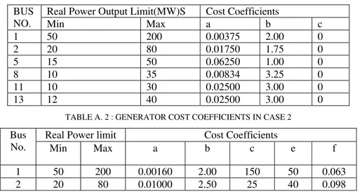
TABLE A.1 : GENERATOR COST COEFFICIENTS IN CASE 1

BUS NO.

Real Power Output Limit(MW)S Cost Coefficients

Min Max a b c

1 50 200 0.00375 2.00 0

2 20 80 0.01750 1.75 0

5 15 50 0.06250 1.00 0

8 10 35 0.00834 3.25 0

11 10 30 0.02500 3.00 0

13 12 40 0.02500 3.00 0

TABLE A. 2 : GENERATOR COST COEFFICIENTS IN CASE 2

Bus No.

Real Power limit Cost Coefficients

Min Max a b c e f

1 50 200 0.00160 2.00 150 50 0.063

TABLE A. 3 EMISSION COEFFICIENTS FOR CASE 3

Unit i

1 4.091e-2 -5.554e-2 6.490e-2 2.0e-4 2.857

2 2.542e-2 -6.047e-2 5.638e-2 5.0e-4 3.333

3 4.258e-2 -5.094e-2 4.586e-2 1.0e-6 8.000

4 5.326e-2 -3.550e-2 3.380e-2 2.0e-3 2.000

5 4.258e-2 -5.094e-2 4.586e-2 1.0e-6 8.000