Optimal Load Dispatch Using Ant Lion Optimization
Menakshi Mahendru Nischal
1,
Shivani Mehta
2M.Tech student, DAVIET, Jalandhar1
Assistant Professor, DAVIET, Jalandhar2
Abstract
This paper presents Ant lion optimization (ALO) technique to solve optimal load dispatch problem. Ant lion optimization (ALO) is a novel nature inspired algorithm. The ALO algorithm mimics the hunting mechanism of ant lions in nature. Five main steps of hunting prey such as the random walk of ants, building traps, entrapment of ants in traps, catching preys, and re-building traps are implemented. Optimal load dispatch (OLD) is a method of determining the most efficient, low-cost and reliable operation of a power system by dispatching available electricity generation resources to supply load on the system. The primary objective of OLD is to minimize total cost of generation while honoring operational constraints of available generation resources. The proposed technique is implemented on 3, 6 & 20 unit test system for solving the OLD. Numerical results shows that the proposed method has good convergence property and better in quality of solution than other algorithms reported in recent literature.
Keywords
—ALO; Optimal load dispatch; transmission lossNomenclature:
ai, bi, ci : fuel cost coefficient of ith generator, Rs/MW2 h, Rs/MW h, Rs/h
F(Pg ) : total fuel cost, Rs/h n : number of generators
� : Minimum generation limit of ith generator, MW
� �� : Maximum generation limit of ith
generator, MW
Pl : Transmission losses, MW Pd : Power demand, MW
I.
INTRODUCTION
The operating cost of a power plant mainly depends on the fuel cost of generators and is minimized via optimal load dispatch. Optimal load dispatch(OLD) problem can be defined as determining the least cost power generation schedule from a set of on line generating units to meet the total power demand at a given point of time [1]. The main objective of OLD problem is to decrease fuel cost of generators, while satisfying equality and inequality constraints. In this problem, fuel cost of generation is represented as cost curves and overall calculation minimizes the operating cost by finding a point where total output of generators equals total power that must be delivered plus losses.
In conventional optimal load dispatch, cost function for each generator has been approximately represented by a single quadratic function and is solved using lambda iteration method, gradient-based method,dynamic programming etc. [1]. Generally, these approaches have hitches in finding an overall optimum, usually offering local optimum point only. Furthermore, traditional approaches require
calculating derivatives and certain inspection on derivability and continuity conditions of function belonging to optimization model. To overcome these shortcomings quite a lot of nature based optimization techniques were applied. Particle swarm optimization [2] is one of the famous meta-heuristics applied to solve OLD problem. Other approaches used for solving OLD problems are: evolutionary programming (EPs) [3], tabu search and multiple tabu search (TS, MTS) [4], differential evolution (DE) [5,6], hybrid DE (DEPSO) [7], artificial bee colony algorithm (ABC) [8], simulated annealing [9],biogeography-based optimization [10],genetic algorithms [11], intelligent water drop algorithm[12] ,hybrid harmony search[13] , differential HS (DHS) [14]gravitational search algorithm[15],firefly algorithm[16],hybrid gravitational search[17],cuckoo search (CS) [18],.have been successfully applied to OLD problems.
II.
PROBLEM FORMULATION
The objective function of the OLD problem is to minimize the total generation cost while satisfying the different constraints, when the necessary load demand of a power system is being supplied. The objective function to be minimized is given by the following equation:2
1
(
)
(
)
n
g i gi i gi i
i
F P
a P
b P
c
… (1)The total fuel cost has to be minimized with the following constraints:
1) Power balance constraint
The total generation by all the generators must be equal to the total power demand and system’s real power loss.
� − � − �
=1 ….. (2)
2) Generator limit constraint
The real power generation of each generator is to be controlled within its particular lower and upper operating limits.
� ≤ � ≤ � ��I =1,2,...,ng …..(3)
III.
ANT LION OPTIMIZATION
Ant Lion Optimizer (ALO)[22] is a novel nature-inspired algorithm proposed by SeyedaliMirjalili in 2015.The ALO algorithm mimics the hunting mechanism of ant lions in nature. Five main steps of hunting prey such as the random walk of ants,
building traps, entrapment of ants in traps, catching preys, and re-building traps are implemented.
Ant lions (doodlebugs) belong to class of net winged insects. The lifecycle of ant lions includes two main phases: larvae and adult. A natural total lifespan can take up to 3 years, which mostly occurs in larvae (only 3–5 weeks for adulthood). Ant lions undergo metamorphosis in a cocoon to become adult. They mostly hunt in larvae and the adulthood period is for reproduction. An ant lion larvae digs a cone-shaped pit in sand by moving along a circular path and throwing out sands with its massive jaw.After digging the trap, the larvae hides underneath the bottom of the cone and waits for insects (preferably ant) to be trapped in the pit. The edge of the cone is sharp enough for insects to fall to the bottom of the trap easily.
Once the ant lion realizes that a prey is in the trap, it tries to catch it.
Fig. 1. Cone-shaped traps and hunting behavior of ant lions[22]
Random walks of ants:Random walks are all based on the Eq.4
� = 0, 2 1 −1 , 2 2 −1 ,… …. . , (2 −1) ……(4)
Where cumsum calculates the cumulative sum, n is the maximum number of iteration, t shows the step of random walk and r(t) is a stochastic function defined as follows:
= 1 � > 0.5
0 � ≤0.5 ……(5)
however, above Eq. cannot be directly used for updating position of ants. In order to keep the random walks inside the search space, they are normalized using the following equation (min–max normalization):
� =(� −�)×( − )
( −�) + ……(6) Where ai is the minimum of random walk of ith variable, bi is the maximum of random walk in ith variable, is the minimum of ith variable at tth iteration, and indicates the maximum of ith variable at tth iteration
Trapping in ant lion's pits: random walks of ants are affected by antlions’ traps. In order to mathematically model this assumption, the following equations are proposed:
� =� +� ….(7)
=� + …(8)
where � is the minimum of all variables at tth iteration, indicates the vector including the maximum of all variables at tth iteration, � is the minimum of all variables for ith ant, is the maximum of all variables for ith ant, and Antliont j shows the position of the selected j-thantlion at tthiteration
during optimization. This mechanism gives high chances to the fitter ant lions for catching ants.
Sliding ants towards ant lion:With the mechanisms proposed so far, ant lions are able to build traps proportional to their fitness and ants are required to move randomly. However, ant lions shoot sands outwards the center of the pit once they realize that an ant is in the trap. This behavior slides down the trapped ant that is trying to escape. For mathematically modelling this behavior, the radius of ants' random walks hyper-sphere is decreased adaptively. The following equations are proposed in this regard:
� = …(9)
= …(10)
where I is a ratio, ct is the minimum of all variables at t-th iteration, and dt indicates the vector including the maximum of all variables at t-th iteration.
Catching prey and re-building the pit:The final stage of hunt is when an ant reaches the bottom of the pit and is caught in the antlion’s jaw. After this stage, the antlion pulls the ant inside the sand and consumes its body. For mimicking this process, it is assumed that catching prey occur when ants becomes fitter (goes inside sand) than its corresponding antlion. An antlion is then required to update its position to the latest position of the hunted ant to enhance its chance of catching new prey. The following equation is proposed in this regard:
� =� � > …(11)
where t shows the current iteration, Antliont j shows the position of selected j-thantlion at t-th iteration, and Antti indicates the position of i-th ant at t-th iteration.
Elitism: Elitism is an important characteristic of evolutionary algorithms that allows them to maintain the best solution(s) obtained at any stage of
optimization process. Since the elite is the fittest antlion, it should be able to affect the movements of all the ants during iterations. Therefore, it is assumed that every ant randomly walks around a selected antlion by the roulette wheel and the elite simultaneously as follows:
� =��+��
2 … (12) where�� is the random walk around the antlion selected by the roulette wheel at t-th iteration, ��is the random walk around the elite at t-th iteration, and � indicates the position of i-th ant at t-th iteration
IV.
RESULTS & DISCUSSIONS
ALO has been used to solve the OLD problems in three different test cases for exploring its optimization potential, where the objective function was limited within power ranges of the generating units and transmission losses were also taken into account. The iterations performed for each test case are 500 and number of search agents (population) taken in both test cases is 30.1) Test system I: Three generating units
The input data for three generators and loss coefficient matrix Bmn is derived from reference [19] and is given in table 4.1.
Table 4.1: Generating unit data for test case I
Unit ai bi ci ���� �����
1 0.03546 38.30553 1243.531 1
35 210
2 0.02111 36.32782 1658.569 6
130 325
3 0.01799 38.27041 1356.659 2
125 315
Bmn=
0.000071 0.000030 0.000025 0.000030 0.000069 0.000032 0.000025 0.000032 0.000080
Table 4.1: Optimal load dispatch for 3 unit system
Without Loss With Loss
Power Demand
(MW) 400 500 600 400 500 600
P1 75.724 97.225 118.73 82.078 105.88 130.02
P2 174.04 210.16 246.28 174.99 212.73 250.85
P3 150.23 192.62 235 150.5 193.31 236.44
Power loss - - - 7.568125 11.91438 17.30402
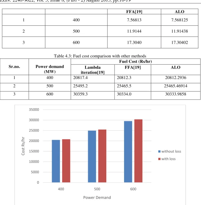
Cost(Rs/hr) 20480.29
695 24924.12631 29520.44334 20812.2936 25465.4691 30333.9858
Table 4.2: Power loss comparison
FFA[19] ALO
1 400 7.56813 7.568125
2 500 11.9144 11.91438
3 600 17.3040 17.30402
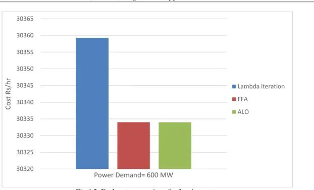
Table 4.3: Fuel cost comparison with other methods
Sr.no. Power demand (MW)
Fuel Cost (Rs/hr) Lambda
iteration[19]
FFA[19] ALO
1 400 20817.4 20812.3 20812.2936
2 500 25495.2 25465.5 25465.46914
3 600 30359.3 30334.0 30333.9858
Fig 4.1. Fuel cost with and without losses for 3 unit system
0 5000 10000 15000 20000 25000 30000 35000
400 500 600
Cos
t
Rs
/h
r
Power Demand
Fig 4.2. Fuel cost comparison for 3 unit system
2) Test system II: Six generating units
The input data for six generators and loss coefficient matrix Bmn is derived from reference [19] and is given in table 4.4.
Table 4.4: Generating unit data for test case II Unit ai bi ci ���� �����
1 0.15240 38.53973 756.79886 10 125 2 0.10587 46.15916 451.32513 10 150 3 0.02803 40.39655 1049.9977 35 225 4 0.03546 38.30553 1243.5311 35 210 5 0.02111 36.32782 1658.5596 130 325 6 0.01799 38.27041 1356.6592 125 315
Bmn=
0.000014 0.000017 0.000015 0.000019 0.000026 0.000022 0.000017 0.000060 0.000013 0.000016 0.000015 0.000020 0.000015 0.000013 0.000065 0.000017 0.000024 0.000019 0.000019 0.000016 0.000017 0.000072 0.000030 0.000025 0.000026 0.000015 0.000024 0.000030 0.000069 0.000032 0.000022 0.000020 0.000019 0.000025 0.000032 0.000085
Table 4.5: Optimal load dispatch for 6 unit system
Without Loss With Loss
Power Demand
(MW) 600 700 800 600 700 800
P1 21.19 24.974 28.758 23.8713 28.3031 32.6003
P2 10 10 10 10 10.00 14.4830
P3 82.086 102.66 123.24 95.6365 118.9550 141.5440
P4 94.371 110.63 126.9 100.7064 118.6728 136.0413
P5 205.36 232.68 260 202.8285 230.7596 257.6587
P6 186.99 219.05 251.1 181.1945 212.7411 243.0033
Power loss - - - 14.2372 19.4317 25.3307
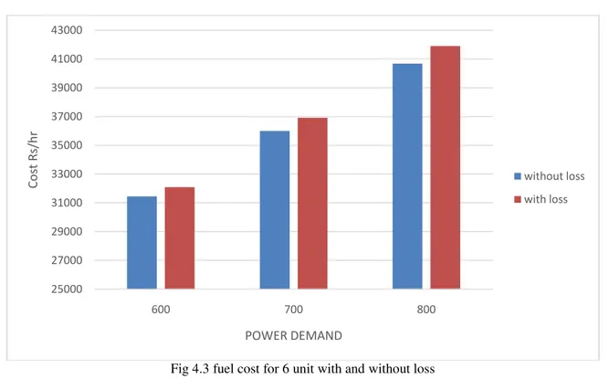
Cost(Rs/hr) 31445.62289 36003.12394 40675.96798 32094.6783 36912.1444 41896.6286
30320 30325 30330 30335 30340 30345 30350 30355 30360 30365
Cos
t
Rs
/h
r
Power Demand= 600 MW
Lambda iteration FFA
Fig 4.3 fuel cost for 6 unit with and without loss
Table 4.6: comparison of power losses.
Sr. no. Power demand Power losses
Conventional[2] PSO[2] FFA[19] ALO
1 600 15.07 14.2374 14.2374 14.2372
2 700 19.50 19.4319 19.4319 19.4317
3 800 25.34 25.3309 25.3312 25.3307
Table 4.7: Comparison of fuel cost with other methods
Sr.no. Power demand
(MW)
Fuel Cost (Rs/hr) Conventional
Method[2]
PSO[2] Lambda iteration[19]
FFA[19] ALO
1 600 32096.58 32094.69 32129.8 32094.7 32094.6783
2 700 36914.01 36912.16 36946.4 36912.2 36912.1444
3 800 41898.45 41896.66 41959.0 41896.9 41896.6286
25000 27000 29000 31000 33000 35000 37000 39000 41000 43000
600 700 800
Cos
t
Rs
/h
r
POWER DEMAND
Fig 4.4. Fuel cost comparison for 6 unit system
3) Test system III: Twenty generating units
The input data for six generators and loss coefficient matrix Bmn is derived from reference [20] and is given in table 4.8.
Table 4.8: generating data for 20 units
Unit ai($/MW2) bi ($/MW) ci ($) ���� �����
1 0.00068 18.19 1000 150 600
2 0.00071 19.26 970 50 200
3 0.00650 19.80 600 50 200
4 0.00500 19.10 700 50 200
5 0.00738 18.10 420 50 160
6 0.00612 19.26 360 20 100
7 0.00790 17.14 490 25 125
8 0.00813 18.92 660 50 150
9 0.00522 18.27 765 50 200
10 0.00573 18.92 770 30 150
11 0.00480 16.69 800 100 300
12 0.00310 16.76 970 150 500
13 0.00850 17.36 900 40 160
14 0.00511 18.70 700 20 130
15 0.00398 18.70 450 25 185
16 0.07120 14.26 370 20 80
17 0.00890 19.14 480 30 85
18 0.00713 18.92 680 30 120
19 0.00622 18.47 700 40 120
20 0.00773 19.79 850 30 100
41860 41870 41880 41890 41900 41910 41920 41930 41940 41950 41960 41970
Power Demand = 800 MW
Conventional Method PSO
Lambda Iteration FFA
Table 4.9: optimal load dispatch for 20-generating units without loss (PD = 2500 MW)
Unit ALO
P1 600
P2 172.85
P3 50
P4 50.481
P5 95.285
P6 24.17
P7 124.81
P8 50
P9 91.891
P10 44.961
P11 275.5
P12 427.35
P13 123.15
P14 59.795
P15 101.7
P16 36.26
P17 36.342
P18 34.196
P19 71.267
P20 30
Total generation (MW) 2500.00 Total generation cost ($/h) 60160.71425
Table 4.10: optimal load dispatch for 20-generating units withloss (PD = 2500 MW)
Unit BBO [21] LI [20] HM [20] ALO
P1 513.0892 512.7805 512.7804 512.78
P2 173.3533 169.1033 169.1035 169.11
P3 126.9231 126.8898 126.8897 126.89
P4 103.3292 102.8657 102.8656 102.87
P5 113.7741 113.6386 113.6836 113.68
P6 73.06694 73.5710 73.5709 73.568
P7 114.9843 115.2878 115.2876 115.29
P8 116.4238 116.3994 116.3994 116.4
P9 100.6948 100.4062 100.4063 100.41
P10 99.99979 106.0267 106.0267 106.02
P11 148.9770 150.2394 150.2395 150.24
P12 294.0207 292.7648 292.7647 292.77
P13 119.5754 119.1154 119.1155 119.12
P14 30.54786 30.8340 30.8342 30.831
P15 116.4546 115.8057 115.8056 115.81
P16 36.22787 36.2545 36.2545 36.254
P17 66.85943 66.8590 66.8590 66.857
P18 88.54701 87.9720 87.9720 87.975
P19 100.9802 100.8033 100.8033 100.8
P20 54.2725 54.3050 54.3050 54.305
Total generation (MW) 2592.1011 2591.9670 2591.9670 2591.967
Total transmission loss (MW) 92.1011 91.9670 91.9669 91.9662
V.
CONCLUSION
In this paper optimal load dispatch problem has been solved by using ALO. The results of ALO are compared for three ,six and twenty generating unit systems with other techniques. The algorithm is programmed in MATLAB(R2009b) software package. The results displayefficacy of ALO algorithm for solving the optimal load dispatch problem. The advantage of ALO algorithm is its simplicity, reliability and efficiency for practical applications.
References
[1] A.J Wood and B.F. Wollenberg, Power Generation, Operation, and Control, John Wiley and Sons, New York, 1984.
[2] Yohannes, M. S. "Solving optimal load dispatch problem using particle swarm optimization technique." International Journal of Intelligent Systems and Applications (IJISA) 4, no. 12 (2012): 12. [3] Sinha N., Chakrabarti R. and Chattopadhyay
P.K., Evolutionary Programming Techniques for Optimal load dispatch, IEEE Transcations on Evolutionary Computation, 2003,20(1):83~94.
[4] POTHIYA, S., I. NGAMROO, W. KONGPRAWECHNON, Application of Multiple Tabu Search Algorithm to Solve Dynamic Economic Dispatch Considering Generator Constraints, Energy Conversion and Management, Vol. 49(4), 2008, pp. 506-516.
[5] NOMAN, N., H. IBA, Differential Evolution for Optimal load dispatch
Problems, Electric Power System Research, Vol. 78(3), 2008, pp. 1322-1331. 17. [6] PEREZ-GUERRERO, R. E. J. R.
CEDENIO-MALDONADO, Economic
Power Dispatch with Non-smooth Cost Functions using Differential Evolution, Proceedings of the 37th Annual North American, Power Symposium, Ames, Iowa, 2005, pp. 183-190.
[7] SAYAH, S., A. HAMOUDA, A Hybrid Differential Evolution Algorithm based on Particle Swarm optimization for Non-convex Economic Dispatch Problems, Applied Soft Computing, Vol. 13(4), 2013, pp. 1608-1619.
[8] HEMAMALINI, S., S. P. SIMON, Artificial Bee Colony Algorithm for Optimal load dispatch Problem with Non-smooth Cost Functions, Electric Power Components and Systems, Vol. 38(7), 2010, pp. 786-803. [9] Basu, M. "A simulated annealing-based
goal-attainment method for economic emission load dispatch of fixed head hydrothermal power systems." International Journal of Electrical Power & Energy Systems 27, no. 2 (2005): 147-153.
[10] Aniruddha Bhattacharya, P.K. Chattopadhyay, “Solving complex optimal load dispatch problems using biogeography-based optimization”, Expert Systems with Applications, Vol. 37, pp. 36053615, 2010. [11] Youssef, H. K., and El-Naggar, K. M.,
“Genetic based algorithm for security constrained power system economic
62456.55 62456.6 62456.65 62456.7 62456.75 62456.8
Cos
t
$/h
r
Power demand = 2500 MW
dispatch”, Electric Power Systems Research, Vol. 53, pp. 4751, 2000.
[12] Rayapudi, S. Rao. "An intelligent water drop algorithm for solving optimal load dispatch problem." International Journal of Electrical and Electronics Engineering 5, no. 2 (2011): 43-49.
[13] Pandi, V. Ravikumar, and Bijaya Ketan Panigrahi. "Dynamic optimal load dispatch using hybrid swarm intelligence based harmony search algorithm." Expert Systems with Applications 38, no. 7 (2011): 8509-8514
[14] WANG, L., L.-P. LI, An Effective Differential Harmony Search Algorithm for the Solving Non-Convex Optimal load dispatch Problems, Electrical Power and Energy Systems, Vol. 44(1), 2013, pp. 832-843.
[15] Swain, R. K., N. C. Sahu, and P. K. Hota. "Gravitational search algorithm for optimal economic dispatch." Procedia Technology 6 (2012): 411-419.
[16] Yang, Xin-She, SeyyedSoheil Sadat Hosseini, and Amir HosseinGandomi. "Firefly algorithm for solving non-convex economic dispatch problems with valve loading effect." Applied Soft Computing 12, no. 3 (2012): 1180-1186
[17] Dubey, Hari Mohan, ManjareePandit, B. K. Panigrahi, and MugdhaUdgir. "Optimal load dispatch by Hybrid Swarm Intelligence Based Gravitational Search Algorithm." International Journal Of Intelligent Systems And Applications (Ijisa) 5, no. 8 (2013): 21-32
[18] Bindu, A. Hima, and M. Damodar Reddy. "Optimal load dispatch Using Cuckoo Search Algorithm." Int. Journal Of Engineering Research and Apllications 3, no. 4 (2013): 498-502.
[19] K. Sudhakara Reddy, Dr. M. Damodar Reddy. “Optimal load dispatch Using Firefly Algorithm.”International Journal of Engineering Research and Applications 2,no.4(2012):2325-2330
[20] C.-T. Su and C.-T. Lin, “New approach with a Hop fi OLD modeling framework to economic dispatch,” IEEE Trans. Power Syst., vol. 15, no. 2, p. 541, May 2000. [21] Bhattacharya, P.K. Chatt opadhyay,
“Biogeography-based optimization for different optimal load dispatch problems,” IEEE Trans. on Power Systems, Vol. 25, pp. 1064- 1077, May 2010.
![Fig. 1. Cone-shaped traps and hunting behavior of ant lions[22]](https://thumb-eu.123doks.com/thumbv2/123dok_br/18268538.344244/2.893.121.780.467.747/fig-cone-shaped-traps-hunting-behavior-ant-lions.webp)