Simulating the binary variates for the components of a socio - economical system

economical system

Ştefan V. Ştefănescu1∗

1

Research Institute for Quality of Life, Romanian Academy; stefanst@fmi.unibuc.ro

Abstract

Often in practice the components Wj of a sociological or an economical system W take discrete 0-1 values. We talk about how to generate arbitrary observations from a binary 0-1 system B when is known the multidimensional distribution of the discrete random vector B. We also simulated a simplified structure of B given by the marginal distributions together with the matrix of the correlation coefficients. Different properties of the systems W are presented too.

Keywords: binary system, marginal distribution, Monte Carlo simulation, random variates, correlation coefficient.

1. Introduction

A general system W with k components W₁,W₂,W₃,...,W_k is characterized by the features λj of every

variable Wj and the intensity cij of the relation between any two components Wi and Wj, 1≤i,j≤k.

Frequently in practice the relation among the elements of the subsystem {W_i,W_j} is a symmetric one, that is

ji ij c c = .

The characteristic λj of the component Wj could be just the parameters which define the marginal

distribution of the random variable Wj. In the following we will choose the Pearson correlation coefficient

) , (W_iW_j

Cor to measure the intensity cij of the relation which is present between the components Wi and Wj of the system W. We mention here that in the literature there are known many other indicators to measure the ratio among the elements Wi and Wj from W ( [1], [2], [6] ).

Figure 1 presents some kinds of systems W.

Many times in practice the system W has components W_j with a normal distribution. Such a system will be designated in the subsequent by X. For this particular case the system components X_j, 1≤ j≤k, are

dependent normal random variables characterized by their means µ_j and their dispersions σ2_j. So we will

take λ_j =(µ_j,σ_j) and c_ij =Cor(X_i,X_j), 1≤i,j≤k.

Another class from the systems W are binary 0-1 systems designated by B. The elements B₁,B₂,B₃,...,B_k of the system B are binary dependent variables which take only the values 0 and 1. To make a distinction between the systems B and X we will use the notation r_ij =Cor(B_i,B_j) in the discrete case and

) , ( _{i j}

ij Cor X X

c = for the continuous normal marginals variant.

We mention here that the normal type system X is completely characterized by the set of the parameters

ij i i,σ ,c

µ , 1≤i<j≤k, that is k(k+3)/2 values ( [3] ) .

But the multidimensional distribution of an arbitrary binary system B has more parameters. For this reason, in opposition with the normal distributions case, we can not define a general binary 0-1 system B by

knowing only the values µi,σi,rij, 1≤i< j≤k. More, in the discrete case of B, the variance σ2j =Var(Bj)

depends on the mean µ_j =Mean(B_j). So, knowing only the marginals and the correlation matrix of B we lose a lot of information which define the real multivariate discrete distribution of the system B. Some details concerning the behavior of a binary system B will be given in the next section.

Fig. 1. A system W with k components

We reveal a new other aspect which is present for sociological and economical systems too. So, the individuals of a given population estimate the behaviour of each component W_j from a continuous system W

by putting subjective marks.

In this approach a binary system B results from W when the marks take only 0 and 1 values. Hence, in practice, we often approximate a continuous system W by a binary one, like B. In this case we must evaluate the discretization error.

2. The binary 0-1 systems

The binary random vector B=(B₁,B₂,B₃,...,B_k) which takes only 0 and 1 values is completely

characterized by the probabilities pi1,i2,i3,...,i_k, ij∈{0,1}, 1≤ j≤k, where

) ,

... , , ,

( 1 1 2 2 3 3

, ... , , ,_{2 3}

1 i i i k k

i Pr B i B i B i B i

p

k = = = = =

Obviously, _{, , ,...,} 0 3

2

1i i ik ≥

i

p _{for all indices} i_j∈{0,1} and in addition

∑ ∑ ∑ ∑

= =

= =

= =

=

=

1

0 1

0 1

0 1

0

, ... , , ,

1

1 2

2 3

3

3 2

1 1

...

i

i i

i i

i i

i

i i i i

k

k

k

p (1)

k j j k j j k j

j i i i i i i i i i i

i

i p p

p _{,..., , , ,..., ,..., ,0, ,..., ,..., ,1, ,...,} 1 1 1 1 1 1 1 1

1 − + + = − + + − +

So, the equality (1) could be also written in a shorter form as p_+,+,+,...,+ =1.

The marginal distributions of the random vector B are defined only by the probabilities q_j =Pr(B_j =1),

k j≤

≤

1 .

Choosing, for example, the component B₁ we deduce

1 1 , ... , , , 1 , ... , , , 0

1 0) 1 1 ( 1) 1

(B p p Pr B q

r

P = = _{++ +}= − _{++ +}= − = = −

Remark 1. Since the distribution of the system B=(B₁,B₂,B₃,...,B_k) is determined by the probabilities

k i i i i

p _{, , ,...,} 3 2

1 with the restriction (1) we conclude that a general binary 0-1 system B with k components is defined by 2k −1 parameters.

Now we will enumerate some properties of a binary B=(B₁,B₂) system which has only two components.

We remind that the distribution of an arbitrary 0-1 binary vector B=(B₁,B₂) is given by the probabilities

) ,

( _{1 2}

, Pr B i B j

p_{i j} = = = where i,j∈{0,1} and p_+,+=1

In this case q₁= p_1,+=Pr(B₁=1) , q₂ =p_+,1=Pr(B₂=1) , 0≤q₁,q₂ ≤1 and therefore

1 , 1 1 0 ,

1 q p

p = −

, p0,1=q2−p1,1, p0,0 =1+ p1,1−q1−q2 Hence we have the inequalities

P2.1. max{0,q1+q2−1}≤min{q1,q2}

After a straightforward calculus we obtain the relations

P2.2. Mean(Bj)=Mean(Bj)=qj

2

, Var(Bj)=qj(1−qj), j∈{0,1}

) 1 ( ) 1 ( ) , ( 2 2 1 1 2 1 1 , 1 2 1 12 q q q q q q p B B Cor r − − − = =

, 0<q₁,q₂ <1

Remark 2. This expression of the correlation coefficient r₁₂=Cor(B₁,B₂) does not depend on the concrete values of the binary random variables B1 and B2. For example, considering B1∈{a1,b1}≠{0,1},

} 1 , 0 { } , { _{2 2}

2∈ a b ≠

B we obtain the same value for the indicator r12.

Since q₁= p_1,0+p_1,1 and q₂ =p_0,1+p_1,1 we prove easily

P2.3. If p_1,1=q₁q₂ then we have also the following equalities

2 1 1

,

0 (1 q )q

p = −

, p1,0=q1(1−q2), p0,0=(1−q1)(1−q2) From P2.2 and P2.3 it results

P2.4. The binary 0-1 random variables B₁, B₂ are independent if and only if r₁₂=Cor(B₁,B₂)=0.

Remark 3. The property P2.4 is not always true for an arbitrary continuous two component system )

, (W₁W₂ W= .

Applying the propositions P2.1 and P2.2 we deduce the inequalities

) 1 ( ) 1 (

} , { )

, (

2 2 1 1

2 1 2 1 2

1

q q q q

q q q q in m B

B Cor

− −

− ≤

, 0<q₁,q₂ <1

The following properties are particular cases of the proposition P2.5.

P2.6. If q1=q2 _then Cor(B1,B2)≤1

If q1=1 q− 2 _then Cor(B1,B2)≥−1

Using the formulas

) , ( )

, 1

( B₁ B₂ Cov B₁ B₂ Cov − =−

, Var(1−B1,B2)=Var(B1,B2)

we can prove directly the equalities

P2.7. Cor(1−B1,B2)=Cor(B1,1−B2)=−Cor(B1,B2)

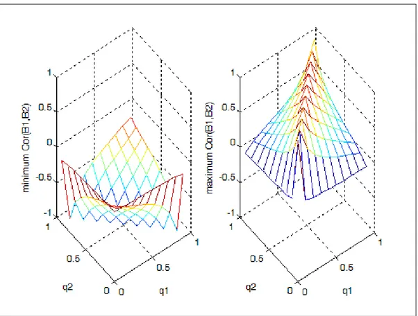
Graphic 1 presents us a suggestive image of the variation for the lower and upper bounds of

) , ( _{1 2}

12 Cor B B

r = index depending on the marginal distributions indicators 0<q₁,q₂<1.

Remark 4. From the propositions P2.1-P2.7 we conclude that the discrete distribution of the system )

, (B₁ B₂

B= is completely determined by the indices 0<q₁,q₂<1 which characterize the marginal distributions of B together with the correlation coefficient r₁₂=Cor(B₁,B₂), −1≤r₁₂≤1. But the parameters

12 2 1,q ,r

q are mutually dependent (see the properties P2.1 and P2.5 or Graphic 1 ).

3. Generate random observations from a binary system

Leisch, Weingessel and Hornik suggested in [5] the application of the general inverse method for discrete random vectors ( [3], [4] ) to generate arbitrary observations (b₁,b₂,b₃,...,b_k), b_j∈{0,1}, for the system

) , ... , , ,

(B₁ B₂ B₃ B_k

B= .

The following algorithm GDRV produces (b₁,b₂,b₃,...,b_k) vectors, b_j∈{0,1}, such that

k

b b b b k

k b p

B b B b B b B r

P _{1 1 2 2 3 3 , , ,...,}

3 2 1 ) ,

... , ,

,

( = = = = =

where the probabilities

k

i i i i

p _{, , ,...,} 3 2

1 , ij∈{0,1}, 1≤ j≤k, define the binary 0-1 system B.

Algorithm GDRV ( Generating Discrete Random Vectors ).

Step 0. Input : the probabilities pi1,i2,i3,...,i_k, ij∈{0,1}, 1≤ j≤k, with p+,+,+,...,+=1.

Step 1. Establish a one to function h:{1,2,3,...,2k}→{0,1}k

Step 2. Compute recurrently the sums

s₀ =0

s_t =s_t−1+p_h(t), _1≤t≤2k

Step 3. Generate a random variate u uniformly distributed on the interval (0,1]

Step 4. Find the index 1≤t≤2k such that u∈(s_t−1,s_t]

Step 5. b=h(t)

Step 6. Output : b

Details regarding the theoretical justification of the generating procedure GDRV can be found in the books [3] and [4].

Remark 5. Applying algorithm GDRV we generated n=106 random variates (b₁,b₂,b₃) from the binary

system B=(B₁,B₂,B₃) defined by Table 1. For this case the frequences of the categories (i₁,i₂,i₃), i_j∈{0,1},

3

1≤ j≤ , are given in Table 2. The validity of the algorithm GDRV is proved in part since the theoretical values and the empirical estimations of the probabilities

3 2 1,i ,i

i

p are very closed ( compare the results from

Tables 1-2 ).

Table 1. The theoretical distribution of the binary 0-1 system B=(B₁,B₂,B₃)

0 , 0 , 0

p p_0,0,1 p_0,1,0 p_0,1,1 p_1,0,0 p_1,0,1 p_1,1,0 p_1.1.1

0.050 0.200 0.100 0.150 0.100 0.050 0.050 0.300

Table 2. The frequences for the variates (b₁,b₂,b₃) obtained after 106 simulations with algorithm GDRV

) 0 , 0 , 0

( (0,0,1) (0,1,0) (0,1,1) (1,0,0) (1,0,1) (1,1,0) (1,1,1)

4. Systems with normal distributed components

Now we will discuss the case of a system X=(X₁,X₂,X₃,...,X_k) where its components X_j, 1≤ j≤k, are random variables with normal distributions.

By X ~Norm(µ,σ2) with µ∈R, σ >0, we understand that the random variable X is normal distributed where Mean( X)=µ and Var(X)=σ2. We denote by Φ(x) the Laplace function, that is the cumulative distribution function for the random variable Z~ Norm(0,1).

Remind some properties which will be applied in the subsequent.

P4.1. If Z~ Norm(0,1) and X=µ+σZ with µ∈R, σ >0 then we have X ~Norm(µ,σ2).

P4.2 ( Inverse method, [3], [4] ). If the random variable U is uniformly distributed on the interval [0,1]

and Z=Φ−1(U) then Z~ Norm(0,1).

P4.3. For any µ_i∈R, σ_i>0, if X_i ~Norm(µ_i,σ_i2) and Y=X₁+X₂ then Y~Norm(µ₁+µ₂,σ₁2+σ₂2).

Discretization procedure DP. For any a∈R, µ∈R, σ >0 and X~Norm(µ,σ2) we designate by B_X,a the

following binary 0-1 random variable

  

≥ < =

a X when

a X when B_{X a}

, 1

, 0

,

Using the procedure DP we deduce by a direct calculus

P4.4. For any X~Norm(µ,σ2) we have Pr(B_X.a=1)=1−Φ((a−µ)/σ)

P4.5. For any −1≤c≤1, Z_i ~ Norm(0,1), the standard normal random variables Z1, Z2 being independent, if

1

Z X =

2 2

1 1 c Z

Z c

Y= + −

then X ~ Norm(0,1), Y ~ Norm(0,1) and more Cor(X,Y)=c.

Remark 6. By using a normal random variable X ~Norm(µ,σ2) and a given bound a∈R we build a

binary 0-1 random variable B_X,a such that ) / ) (( 1 ) 1 (

Pr _. = = −Φ −µ σ

= B a

q _Xa

( see the discretization procedure DP and Proposition P4.4 ). When µ=0 and σ =1, the threshold a∈R

determine effectively the distribution of the discrete 0-1 random variable B_X,a.

5. A discretization process

Having a continuous normal distributed system X=(X₁,X₂,X₃,...,X_k) and fixing some arbitrary thresholds a₁,a₂,a₃,...,a_k∈R we can obtain a binary 0-1 system B=(B₁,B₂,B₃,...,B_k) with

j j a

X j B B = _, ,

k j≤ ≤

1 ( apply the procedure DP ).

Obviously, in this last case, the correlation indicators r_ij =Cor(B_i,B_j) and c_ij =Cor(X_i,X_j), 1≤i,j≤k,

have not equal values. More precisely, a correlation coefficient rij depends on the quantities cij,qi,qj. The

effective relation between rij and cij indices will be established in the subsequent by applying a stochastic

Monte Carlo simulation.

Remark 7. For an arbitrary −1≤c≤1, propositions P4.2 and P4.5 permit us to generate two dependent

standard normal random variables X ,Y having just the Pearson correlation coefficient Cor(X,Y)=c. We can apply Proposition P4.2 ( the inverse method, [3], [4] ) to generate independent Z_i ~ Norm(0,1) random variables which are used by Proposition P4.5.

Now, keeping all the previous notations, we will suggest a Monte Carlo procedure MCRCC to establish the real ratios between he correlation coefficients c_ij=Cor(X_i,X_j) and r_ij=Cor(B_i,B_j).

Procedure MCRCC.

Step 1. We generate random variates of volume n for a bidimensional random vector (X₁,X₂) with standard normal dependent marginals and c₁₂=Cor(X₁,X₂), −1≤c₁₂≤1 ( more details in Remark 7 ).

Step 2. Knowing the marginal probabilities −1≤q₁,q₂ ≤1, we specify the discretization thresholds, that is a₁=Φ−1(1−q₁), a₂=Φ−1(1−q₂).

Step 3. We obtain 0-1 binary samples (b₁,b₂) from the random vector B=(B_i,B_j) considering the discretization procedure

1 1,

1 BX a

B = ,

2 2,

2 BX a

B = ( algorithm DP ).

Step 4. Using the samples resulted for B=(B_i,B_j) we estimate the correlation coefficient

) , ( _{1 2}

12 Cor B B

r = .

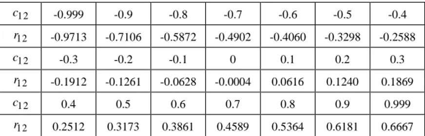
The correlation values r₁₂ from Tables 3-5 were deduced by running the Monte Carlo algorithm MCRCC

for samples having the volume n=107.

Table 3. q₁=q₂=0.5, n=107 Monte Carlo simulations with MCRCC

12

c -0.999 -0.9 -0.8 -0.7 -0.6 -0.5 -0.4

12

r -0.9714 -0.7129 -0.5906 -0.4938 -0.4099 -0.3335 -0.2621

12

c -0.3 -0.2 -0.1 0 0.1 0.2 0.3

12

r _{-0.1940 -0.1282 -0.0637 0.0001 0.0638 0.1284 0.1943}

12

c _{0.4 0.5 0.6 0.7 0.8 0.9 0.999}

12

r _{0.2622 0.3333 0.4096 0.4937 0.5904 0.7129 0.9714}

Table 4. q₁=0.4, q₂=0.6, n=107 simulations with MCRCC

12

c _{-0.999 -0.9 -0.8 -0.7 -0.6 -0.5 -0.4}

12

r _{-0.9713 -0.7106 -0.5872 -0.4902 -0.4060 -0.3298 -0.2588}

12

c _{-0.3 -0.2 -0.1 0 0.1 0.2 0.3}

12

r -0.1912 -0.1261 -0.0628 -0.0004 0.0616 0.1240 0.1869

12

c 0.4 0.5 0.6 0.7 0.8 0.9 0.999

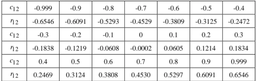
Table 5. q₁=0.5,q₂=0.7 , _n=107 _{simulations with MCRCC}

12

c _{-0.999 -0.9 -0.8 -0.7 -0.6 -0.5 -0.4}

12

r _{-0.6546 -0.6091 -0.5293 -0.4529 -0.3809 -0.3125 -0.2472}

12

c _{-0.3 -0.2 -0.1 0 0.1 0.2 0.3}

12

r -0.1838 -0.1219 -0.0608 -0.0002 0.0605 0.1214 0.1834

12

c 0.4 0.5 0.6 0.7 0.8 0.9 0.999

12

r 0.2469 0.3124 0.3808 0.4530 0.5297 0.6091 0.6546

Remark 8. The differences between the correlation values r₁₂=Cor(B₁,B₂) and c₁₂=Cor(X₁,X₂) are sometimes considerable. Graphic 2 gives us a suggestive illustration of this aspect ( compare the differences between the continuous and dotted curves ).

Graphic 2. The ratio between the correlation indices r₁₂ and c₁₂

Remark 9. We can use successively Proposition P4.5 and the discretization procedure DP to simulate

directly samples from a tree type binary systems. See, for example, the one level tree system depicted in

Figure 1, case 1.3.

6. Concluding remarks

We discussed two algorithms to generate random variates for a binary system B=(B₁,B₂,B₃,...,B_k) with k components.

The algorithm GDRV uses as inputs all the probabilities pi₁,i₂,i₃,...,i_k, ij∈{0,1}, 1≤ j≤k, which

characterize the binary system B. It is not so easy to apply practically the procedure GDRV for systems B

For this reason is suggested a new other algorithm based on the discretization procedure DP to obtain arbitrary observations from B. This procedure simulate better the real aspects. The correlation structure of a continuous system X is inherited by the binary system B resulted after a discretization process. The relation between the correlation coefficients c₁₂=Cor(X₁,X₂) and r₁₂=Cor(B₁,B₂) can be determined by applying

MCRCC algorithm ( see also Graphic 2 ).

References

[1] Agresti, A., An introduction to categorical data analysis, John Wiley and Sons, New York, 1996. [2] Andersen, E.B., Introduction to the statistical analysis of categorical data, Springer, New York, 1997. [3] Devroye, L., Non-uniform random variate generation, Springer-Verlag, New York, 1986.

[4] James E. Gentle, J.E., Random number generation and Monte Carlo methods, Springer - Statistics and Computing, New York, (second edition), 2003.

[5] Leisch, F., Weingessel, A., Hornik, K., “On the generation of correlated artificial binary data”, Adaptive Information Systems and Modelling in Economics and Management Science, Working Paper Series SFD, no. 13, Vienna University of Economics, 1998.