Available online at www.ispacs.com/jiasc Volume 2014, Year 2014 Article ID jiasc-00033, 18 Pages
doi:10.5899/2014/jiasc-00033 Research Article
A Numerical Approach for Solving Optimal Control Problems
Using the Boubaker Polynomials Expansion Scheme
B. Kafash1∗, A. Delavarkhalafi1, S. M. Karbassi2, K. Boubaker3
(1)Faculty of Mathematics, Yazd University, Yazd, P.O. Box 89197/741, Iran.
(2)Faculty of Advanced Education, Islamic Azad University, Yazd Branch, Yazd, Iran
(3)Unite de physique des dispositifs´ a semi-conducteurs, Facult` e des sciences de Tunis, Tunis El Manar University, 2092 Tunis, Tunisia.´ Copyright 2014 c⃝B. Kafash, A. Delavarkhalafi, S. M. Karbassi and K. Boubaker. This is an open access article distributed under the Creative Commons Attribution License, which permits unrestricted use, distribution, and reproduction in any medium, provided the original work is properly cited.
Abstract
In this paper, we present a computational method for solving optimal control problems and the controlled Duffing oscillator. This method is based on state parametrization. In fact, the state variable is approximated by Boubaker polynomials with unknown coefficients. The equation of motion, performance index and boundary conditions are converted into some algebraic equations. Thus, an optimal control problem converts to a optimization problem, which can then be solved easily. By this method, the numerical value of the performance index is obtained. Also, the control and state variables can be approximated as functions of time. Convergence of the algorithms is proved. Numerical results are given for several test examples to demonstrate the applicability and efficiency of the method.
Keywords:Optimal control problems; Controlled linear and Duffing oscillator; Boubaker polynomials expansion scheme (BPES); optimization problem; Weierstrass approximation theorem.
1 Introduction and Preliminaries
Optimal control problems play an important role in a range of application areas including engineering, economics and finance. Control Theory is a branch of optimization theory concerned with minimizing a cost or maximizing a payout pertaining. An obvious goal is to find an optimal open loop controlu∗(t)or an optimal feedback control u∗(t,x)that satisfies the dynamical system and optimizes in some sense performance index. There are two general methods for solving optimal control problems. These methods are labeled as direct and indirect methods.
An indirect method transforms the problem into another form before solving it and can be grouped into two categories: Bellman’s dynamic programming method and Pontryagin’s Maximum Principle. Bellman pioneered work in dynamic programming which led to sufficient conditions for optimality using the Hamilton-Jacobi-Bellman (HJB) equations. In fact, a necessary condition for an optimal solution of optimal control problems is the HJB equation. It is a second-order partial differential equation which is used for finding a nonlinear optimal feedback control law. Pontryagin’s Maximum Principle is used to find the necessary conditions for the existence of an optimum. This convert the original optimal control problem into a boundary value problem, which can be solved by using well known techniques for differential equations, analytically or numerically (for details see [1, 2, 3, 4, 5, 6]). As analytical solutions of optimal
control problems are not always available, therefore, finding a numerical solution for solving optimal control prob-lems is at least the most logical way to treat them and has provided an attractive field for researchers of mathematical sciences. In recent year, different numerical computational methods and efficient algorithms have been used to solve the optimal control problems (for example see [7, 8, 9, 10, 11, 12, 13, 14]).
In direct methods, the optimal solution is obtained by direct minimization of the performance index subject to con-straints. In fact, the optimal control problems can be converted into a optimization problem. The direct methods can be employed by using the parameterizations technique which can be applied in three different ways: control parame-terizations, control-state parameterizations and state parameterizations [15, 16, 17, 18]. State parametrization converts the problem to a nonlinear optimization problem and finds unknown polynomial coefficients of degree at mostnin the form of∑ki=0aitifor optimal solution [19, 20]. The control parameterizations and control-state parameterizations have been used extensively to solve general optimal control problems. Jaddu has presented numerical methods to solve un-constrained and un-constrained optimal control problems [17] and later, extended his ideas to solve nonlinear optimal control problems with terminal state constraints, control inequality constraints and simple bounds on state variables [18]. In [21, 22], the authors have presented a numerical technique for solving nonlinear constrained optimal control problems. Gindy has presented a numerical solution for solving optimal control problems and the controlled Duffing oscillator, using a new Chebyshev spectral procedure [23]. In [24], the authors have presented a spectral method of solving the controlled Duffing oscillator. In [25], a numerical technique is shown for solving the controlled Duffing oscillator; in which the control and state variables are approximated by Chebyshev series. In [26], an algorithm for solving optimal control problems and the controlled Duffing oscillator is presented; in the algorithm the solution is based on state parametrization such that the state variable can be considered as a linear combination of Chebyshev polynomials with unknown coefficients and later, extended state parametrization to solve nonlinear optimal control problems and the controlled Duffing oscillator [27].
This paper is organized into following sections of which this introduction is the first. In Section 2, we introduce math-ematical formulation. Section 3 is about Boubaker polynomials. The proposed design approach and its convergence are derived in Section 4. In section 5 we present a numerical example to illustrate the efficiency and reliability of the presented method. Finally, the paper is concluded with conclusion.
2 Problem statement
Optimal control deals with the problem of finding a control law for a given system
˙
x(t) =f(t,x(t),u(t)), t∈I◦, (2.1) where,f is a real-valued continuously differentiable function,f:I×E×U→Rn. AlsoI= [t0,t1]for the time interval, u(t):I→Rnfor the control andx(t):I→Rmfor the state variable is used. As the control function is changed, the solution to the differential equation will be changed. The subject is to find a piecewise continuous controlu∗and the associated state variablex∗(t)that optimizes in some sense the performance index
J(t0,x0;u) =
∫ t1
t0
L(t,x(t),u(t))dt, (2.2)
subject to (2.1) with boundary conditions
x(t0) =x0 and x(t1) =x1, (2.3) where, x0 andx1are initial and final state in Rn; respectively, that may be fixed or free. Control u∗is called an optimal controland state variablex∗anoptimal trajectory. Also,L:I×E×U→Ris assumed to be a continuously differentiable function in all three arguments. the optimization problem with performance index as in equation (2.2) is called aLagrangeproblem. There are two other equivalent optimization problems, which are calledBolzaandMayer problems [2]. Particularly in optimal control problemsLcan be an energy or fuel function as below [28]:
L(t,x(t),u(t)) = 1 2(x
2(t) +u2(t))
,
Generally,Jmay be a multi purpose or multi objective functional; for example, in minimization of fuel dissipation or maximization of benefit.
Example 2.1. Linear quadratic optimal control problem
A large number of design problems in engineering is an optimization problem. This problem is called the linear regulator problem. Let A(t), M(t)and D be n×n matrices and B(t), n×m and N(t), m×m, matrices of continuous functions. Let u(t)be defined on a fixed interval[t0,t1], which is an m−dimensional piecewise continuous vector function. The state vector x(t)∈Rnis the corresponding solution of initial value problem
˙
x=A(t)x(t) +B(t)u(t), x(t0) =x0. (2.4) The optimal control problem is to find an optimal control u(t)which minimizes the performance index,
J=x(t1)′Dx(t1) +
∫ t1
t0 (
x(t)′M(t)x(t) +u(t)′N(t)u(t))
dt. (2.5)
Here M(t), N(t)and D are symmetric with M(t)and D non negative definite and N(t)positive definite matrices. Let x= (x1,x2,···,xn)′then the Hamilton-Jacobi-Bellman equation with the final condition will be
(HJB) {
Vt+minu∈U {
Vx(Ax+Bu)+(x′Mx+u′Nu) }
=0,
V(t1,x) =x′Dx.
In the case of linear quadratic optimal control problem (2.4)-(2.5), if the value V(t,x) =x′K(t)x is substituted in the HJB equation, where K(t)is a C1symmetric matrix with K(t1) =D, then HJB equation leads to a control law of the form
u(t) =−N−1(t)B(t)′K(t)x(t).
Here K(t)satisfies the matrix Riccati equation [17]
{ ˙
K(t) =−A(t)′K(t)−K(t)A(t) +K(t)B(t)N−1(t)B(t)′K(t)−M(t), K(t1) =D.
Example 2.2. The Controlled Linear Oscillator
We will consider the optimal control of a linear oscillator governed by the differential equation
u(t) =x¨(t) +ω2x(t)
, t∈[−T,0], (2.6)
in which T is specified. equation (2.6) is equivalent to the dynamic state equations
˙
x1(t) = x2(t), ˙
x2(t) = −ω2x1(t) +u(t)
,
with the boundary conditions
x1(−T) =x0 , x2(−T) =x˙0
x1(0) =0 , x2(0) =0. (2.7)
It is desired to control the state of this plant such that the performance index
J=1 2
∫ 0
−T
is minimized over all admissible control functions u(t). Pontryagin’s maximum principle method [5] applied to this optimal control problem yields the following exact analytical solution [22]:
x1(t) = 1
2ω2[Aωtsinωt+B(sinωt−ωtcosωt)], x2(t) = 1
2ω[A(ωtsinωt+ωtcosωt) +Bωtsinωt],
u(t) = Acosωt+Bsinωt,
J = 1
8ω[2ωT(A
2+B2) + (A2−B2)sin 2ωT−4ABsin2ωT],
where
A = 2ω[x0ω
2TsinωT−x˙
0(ωTcosωT−sinωT)]
ω2T2−sin2ωT ,
B = 2ω
2[x˙
0TsinωT+x0(ωTcosωT+sinωT)]
ω2T2−sin2ωT .
The Controlled Duffing Oscillator
Controlled Duffing oscillator described by the nonlinear differential equation
u(t) =x¨(t) +ω2x(t) +εx3(t)
, t∈[−T,0],
Subject to the boundary conditions and with the performance index pointed out as in the previously linear case. The exact solution in this case is not known.
3 The Boubaker polynomials
In this section, Boubaker polynomials, which are used in the next sections, are reviewed briefly. The Boubaker polynomials were established for the first by Boubaker et al. as a guide for solving heat equation inside a physical model. In fact, in a calculation step during resolution process, an intermediate calculus sequence raised an interesting recursive formula leading to a class of polynomial functions that performs difference with common classes (for details see [29, 30, 31, 32, 33, 34]).
Definition 3.1. The first monomial definition of the Boubaker polynomials is introduced by:
Bn(X) =
ζ(n)
∑
p=0 [
(n−4p) (n−p)C
p n−p
]
.(−1)p.Xn−2p,
where
ζ(n) =⌊n
2 ⌋
=2n+ ((−1)
n−1)
4 .
Their coefficients could be defined through a recursive formula
Bn(t) =∑ζ( n)
j=0[bn,jtn−2j], bn,0=1,
bn,1=−(n−4),
bn,j+1=(n(−j+21j)()(nn−−2jj−−11))n−n−4j4−j4.bn,j, bn,ζ(n)=
{
(−1)n2.2 I f n even,
Remark 3.1. A recursive relation which yields the Boubaker polynomials is:
B0(t) =1, B1(t) =t,
B2(t) =t2+2,
Bm(t) =tBm−1(t)−Bm−2(t), For m>2, The ordinary generating functionfB(t,x)of the Boubaker polynomials is:
fB(t,x) =
1+3x2 1+x(x−t). The characteristic differential equation of the Boubaker polynomials is:
Any′′+Bny′−Cny=0. where
An = (x2−1)(3nx2+n−2),
Bn = 3x(nx2+3n−2), Cn = −n(3n2x2+n2−6n+8).
Lemma 3.1. Some arithmetical or integral properties of Boubaker polynomials are as follow:
Bn(0) = 2 cos (
n+2
2 π
)
, n≥1 Bn(−t) = (−1)nBn(t).
4 The proposed design approach
In this section, a new parameterizations using Boubaker polynomials, to derive a robust method for solving optimal control problems numerically is introduced. In fact, we can accurately represent state and control functions with only a few parameters. First, from equation (2.1), the expression foru(t)as a function oft,x(t)and ˙x(t)is determined, i.e. [10]
u(t) =φ(t,x(t),x˙(t)), (4.9)
LetQ⊂C1([0,1])be set of all functions satisfying initial conditions (2.3). Substituting (4.9) into (2.2), shows that performance index (2.2) can be explained as a function ofx. Then, the optimal control problem (2.1)-(2.3) may be considered as minimization ofJon the setQ. The state parametrization can be employed using different basis functions [16]. In this work, Boubaker polynomial will be applied to introduce a new algorithm for solving optimal control problems numerically. LetQn⊂Qbe the class of combinations of Boubaker polynomials of degrees up ton, and consider the minimization ofJonQnwith{ak}nk=0as unknowns. In fact, state variable is approximated as follow:
xn(t) = n
∑
k=0
akBk(t), n=1,2,3,··· (4.10)
The control variables are determined from the system state equations (4.9) as a function of the unknown parameters of the state variables
un(t) =φ(t, n
∑
k=0 akBk(t),
n
∑
k=0
akB˙k(t)). (4.11)
By substituting these approximation of the state variables (4.10) and control variables (4.11) into the performance index (2.2) yield:
ˆ
J(a0,a1, . . . ,an) =
∫ t1
t0
L(t,
n
∑
k=0
akBk(t),φ(t, n
∑
k=0 akBk(t),
n
∑
k=0
Thus, the problem can be converted into a quadratic function of the unknown parametersai. The initial condition is replaced by equality constraint as follow:
xn(t0) = n
∑
k=0 akBk(t)
t=t
0 =x0,
xn(t1) = n
∑
k=0 akBk(t)
t=t1
=x1. (4.13)
The new problem can be stated as:
min a∈Rn+1
{
a′Ha}, (4.14)
subject to constrains (4.13) due to the initial and final conditions, which are linear constrains as:
Pa=b. (4.15)
In fact, this is an optimization problem in (n+1)-dimensional space and J(xn) may be considered as ˆJ(a′) = ˆ
J(a0,a1, . . . ,an), which ˆJ is approximate value ofJ. The optimal value of the vectora∗can be obtained from the standard quadratic programming method.
4.1 An efficient algorithm
The above result is summarized in the following algorithm. The main idea of this algorithm is to transform the optimal control problems (2.1)-(2.3) into a optimization problem (4.14)-(4.15) and then solve this optimization prob-lem.
Algorithm.
Input:Optimal control problem (2.1)-(2.3).
Output:The approximate optimal trajectory, approximate optimal control and approximate performance indexJ.
Step 1.Approximate the state variable bynthBoubaker series from equation (4.10).
Step 2.Find the control variable as a function of the approximated state variable from equation (4.11).
Step 3.Find an expression of ˆJfrom equation (4.12) and find the matrixH.
Step 4.Determine the set of equality constraints, due to the initial and final conditions and find the matrixP.
Step 5. Determine the optimal parametersa∗ by solving optimization problem (4.14)-(4.15) and substitute these
parameters into equations (4.10), (4.11) and (4.12) to find the approximate optimal trajectory, approximate optimal control and approximate performance indexJ, respectively.
4.2 A case study
The next example clarifies the presented concepts: Findu∗(t)that minimizes [17]
J=
∫ 1
0 (
x21+x22+0.0005u2(t)dt, 0≤t≤1, (4.16) subject to
˙
x1 = x2,
˙
x2 = −x2+u, (4.17)
with initial conditions
The first step in solving this problem by the proposed method is by approximatingx1(t)by 5thorder Boubaker series of unknown parameters, we get
x1(t) = 5
∑
k=0
akBk(t) =a5t5+a4t4+ (a3−a5)t3+a2t2+ (a1+a3−3a5)t+a0+2a2−2a4. (4.19)
Then, ˙x1(t)is calculated andx2(t)can be determined,
x2(t) =5a5t4+4a4t3+ (3a3−3a5)t2+2a2t+a1+a3−3a5, (4.20) and then the control variable are obtained from the state equation (4.17), as follows:
u(t) =5a5t4+ (4a4+20a5)t3+ (3a3+12a4−3a5)t2+ (2a2+6a3−6a5)t+a1+2a2+a3−3a5, (4.21) By substituting (4.19)-(4.21) into (4.16), the following expression for ˆJcan be obtained
ˆ
J = a02+a0a1+ 13
3 a0a2+ 3 2a0a3−
18 5 a0a4−
19 6 a0a5+
803 600a1
2+453 100a1a2+
307 60 a1a3+
23 60a1a4
− 5687
700 a1a5+ 1037
150 a2
2+5399 600 a2a3−
12788 2625 a2a4−
1631 120 a2a5+
122539 21000 a3
2+593 150a3a4−
461117 31500 a3a5
+ 45929
7875 a4 2+263
600a4a5+
8841737 693000 a5
2
, (4.22)
which convert to
ˆ
J= [a0a1a2a3a4a5]
1 12 73 34 −9
5 − 19 12 1 2 803 600 453 200 307 120 23 120 − 5687 1400 7 3 453 200 1037 150 5399 1200 − 12877 5250 − 1631 240 3 4 307 120 5399 1200 122539 21000 593 300 − 461117 63000 −9 5 23 120 − 12877 5250 593 300 45929 7875 563 1200 −19 12 − 5687 1400 − 1631 240 − 461117 63000 563 1200 8841737 963000 a0 a1 a2 a3 a4 a5 . (4.23)
From initial conditions (4.18), another equations representing the initial states are obtained as follow:
a0+2a2−2a4=0,
a1+a3−3a5=−1, (4.24)
that means:
[
1 0 2 0 −2 0
0 1 0 1 0 −3
] a0 a1 a2 a3 a4 a5 = [ 0 −1 ] . (4.25)
standard quadratic programming method as: a0 a1 a2 a3 a4 a5 = 100962514997240 12724695632333 1281600273247307 445364347131655 61331171268920 12724695632333 −5637856545538764 445364347131655 111812428767540 12724695632333
−1303630641719934445364347131655 . (4.26)
Now, we calculate state variablesx1(t)andx2(t)approximately as:
x1(t) = −t+
61331171268920 12724695632333t
2
−866845180763766
89072869426331 t
3+111812428767540 12724695632333 t 4 −1303630641719934 445364347131655 t 5 , and
x2(t) = −1+
122662342537840 12724695632333 t−
2600535542291298 89072869426331 t
2+447249715070160 12724695632333 t
3−1303630641719934 89072869426331 t
4, and approximated controlu(t)as:
u(t) =109937646905507 12724695632333 −
4342434686817716 89072869426331 t+
6791708474182062 89072869426331 t 2 − 2083774561388616 89072869426331 t 3 −1303630641719934 89072869426331 t 4 .
Also, by substituting optimal parameters (4.26) into (4.23) the approximate optimal value can be obtained. For the example, the optimal value is obtainedJ=0.0759522. This particular case is also solved by approximatingx1(t)into 9thorder Boubaker series of unknown parameters. The optimal value is obtain to be 0.0693689 which is very close to both the exact value 0.06936094 and the result obtained in [17] using 9thorder Chebyshev series which is 0.0693689
4.3 Convergence analysis
The convergence analysis of the proposed method is based on Weierstrass approximation theorem (1885).
Theorem 4.1. Let f ∈C([a,b],R). Then there is a sequence of polynomials Pn(x)that converges uniformly to f(x)
on[a,b]. Proof. See [35]
Lemma 4.1. Ifαn=inf
Pn
J, for n∈N, where Pnbe a subset of Q, consisting of all polynomials of degree at most n. Then lim
n→∞αn=α whereα=infQ J. Proof.
See [26]
The next theorem guarantees the convergence of the presented method to obtain the optimal performance indexJ(.).
Theorem 4.2. If J has continuous first derivatives and for n∈N,γn=inf
Proof.
If we defineγn=minan∈Rn+1J(an), then:
γn=J(a∗n), a∗n∈Argmin{J(an):an∈Rn+1}. Now let:
x∗n∈Argmin{J(x(t)):x(t)∈Qn}. Then
J(x∗n(t)) = min
x(t)∈QnJ(x(t)),
in whichQnis a class of combinations of Boubaker polynomials int of degree n, so γn=J(xn∗(t)). Furthermore, according toQn⊂Qn+1, we have:
min x(t)∈Qn+1
J(x(t))≤ min x(t)∈Qn
J(x(t)).
Thus, we will haveγn+1≤γnwhich meansγnis a non increasing sequence. Now, according to Lemma 4.1, the proof is complete, that is:
lim
n→∞γn=xmin(t)∈Q J(x(t)).
Note that, this theorem is proved whenQnis a class of combinations of Chebyshev polynomials [26].
5 Numerical examples
To illustrate the efficiency of the presented method, we consider the following examples. All problems considered have continuous optimal controls and can be solved analytically. This allows verification and validation of the method by comparing with the results of exact solutions. Note that, our method is based on state parameterization, so we have compared it with the method given in [20], [26] and [27]. Furthermore, comparison between the exact and the approximate trajectory ofx(t), of controlu(t)and of performance indexJare also presented (see tables 2 and 6 also table 4).
Example 5.1. ([2, 7, 8, 23, 26])
The object is to find the optimal control which minimizes
J=1 2
∫ 1
0 (
u2(t) +x2(t))
dt, 0≤t≤1, (5.27)
when
˙
x(t) =−x(t) +u(t), x(0) =1. (5.28)
We can obtain the analytical solution by the use of Pontryagin’s maximum principle which is [26]:
x(t) =Ae √
2t+ (
1−A)e− √
2t
,
u(t) =A(√2+1)e√2t−(1−A)(√2−1)e−√2t,
and
J=e−
2√2 2
(
(√2+1)(e4√2−1)A2+ (√2−1)(e2√2−1)(1−A)2)
where A= 2√2−3
−e2√2+2√2−3. By approximating x(t)by second order Boubaker series of unknown parameters, we get
x(t) =
2
∑
k=0
akBk(t), (5.29)
and then the control variable are obtained from the state equation (5.28), as follows:
u(t) = +a2t2+ (a1+2a2)t+a0+a1+3a2. (5.30) By substituting (5.29) and (5.30) into (5.27), the following expression forJ can be obtainedˆ
ˆ
J= [a0a1a2]
1 1 176 1 43 134 17
6 13
4 87 10
a0 a1 a2
. (5.31)
From initial condition (5.28), another equation representing the initial states are obtained
a0+2a2=1. (5.32)
The dynamic optimal control problem is approximated by a quadratic programming problem. The new problem is to minimize (5.31) subject to the equality constraint (5.32). The optimal value of the vectora∗ can be obtained from the standard quadratic programming method. By substituting these optimal parameters into (5.31), the approximate optimal value can be calculated. The optimal cost functional J, obtained by the presented method is shown for different n in Table 1.
Table 1: Optimal cost functionalJfor differentnin Example 5.1
n J Error
3 0.1929316056 2.2e−5 4 0.1929094450 1.7e−7 5 0.1929092990 8.6e−10
The exact solution for the performance index is J=0.1929092978. The optimal cost functional, J, obtained by the presented method for n=4is a good approximation. This leads to state and control variables approximately as:
x(t) =1.0−1.38t+0.982t2−0.403t3+0.0871t4,
and
u(t) =−0.384+0.579t−0.227t2−0.0542t3+0.0871t4,
0 0.1 0.2 0.3 0.4 0.5 0.6 0.7 0.8 0.9 1 −0.4
−0.2 0 0.2 0.4 0.6 0.8 1
t
Exact Solution of x(t) x
4(t) Exact Solution of u(t) u
4(t)
Figure 1: Solution of Example 5.1. The approximate solution forn=4 is compared with the actual analytical solution.
Note that, the previous problem is also solved by expanding x(t)into10th order Boubaker series, and the optimal value is obtained0.1929092981which is very close to the exact value J and the result obtained in [20] and [26],
three iterations of their algorithms are0.193828723and0.192909776, respectively. The maximum absolute error of
state variable (∥x(t)−xn(t)∥∞), control variable (∥u(t)−un(t)∥∞) and performance index (|J−Jn|) are listed in Table 2 for different n of presented algorithm.
Table 2: The maximum absolute error of performance index, state and control variables for differentnin Example 5.1 n ∥x(t)−xn(t)∥∞ ∥u(t)−un(t)∥∞ |J−Jˆ|
1 1.2e−1 6.3e−1 5.7e−2 2 9.5e−3 5.5e−2 1.3e−3 3 1.0e−3 8.0e−3 2.2e−5 4 6.4e−5 1.5e−3 1.7e−7
5 4.0e−6 4.8e−5 8.6e−10 6 1.9e−7 7.6e−6 2.3e−12 7 9.3e−9 1.6e−7 7.6e−15 8 3.3e−10 6.8e−9 1.3e−17 9 1.2e−11 2.5e−10 2.4e−20 10 1.1e−11 2.3e−10 2.2e−20
Example 5.2. [3, 27]
The object is to find the optimal control which minimizes
J=1 2
∫ 2
0
u2(t)dt, 0≤t≤2, (5.33)
when
u(t) =x˙(t) +x¨(t), (5.34)
and
x(0) =0, x˙(0) =0, x(2) =5, x˙(2) =2, (5.35)
are satisfied. Where analytical solution is
x(t) =−6.103+7.289t+6.696e−t−0.593et,
and
Therefore, the exact value of performance index is J=16.74543860. By approximating x(t)by third order Boubaker
series of unknown parameters, we get
x(t) =
3
∑
k=0
akBk(t), (5.36)
and then the control variable are obtained from the state equation (5.34), as follow:
u(t) =a1+2a2+a3+ (2a2+6a3)t+3a3t2, (5.37) By substituting (5.37) into (5.33), the following expression forJ can be obtainedˆ
ˆ
J= [a1a2a3]
1 4 11
4 523 52 11 52 8495
a1 a2 a3
. (5.38)
From boundary conditions (5.35), another equations representing the initial states are obtained as follow:
a0+2a2=0,
a0+2a1+6a2+10a3=5, (5.39)
a1+a3=0,
a1+4a2+13a3=2.
The dynamic optimal control problem is approximated by a quadratic programming problem. The new problem is to minimize (5.38) subject to the equality constraint (5.39). The optimal value of the vectora∗ can be obtained from the standard quadratic programming method. By substituting these optimal parameters into (5.38), the approximate optimal value can be calculated. The optimal cost functional J, obtained by the presented method is shown for different n in Table 3.
Table 3: Optimal cost functionalJfor differentnin Example 5.2
n J Error
4 16.76304348 1.8e−2 5 16.75073345 5.3e−3 6 16.75072526 5.2e−3
For n=5we calculate state and control variables approximately as:
x(t) =3.05t2−1.19t3+0.218t4−0.0359t5 and
u(t) =6.09−1.04t−0.957t2+0.152t3−0.180t4,
0 0.2 0.4 0.6 0.8 1 1.2 1.4 1.6 1.8 2 −2
−1 0 1 2 3 4 5 6 7
t
Exact Solution of x(t) x
5(t) Exact Solution of u(t) u5(t)
Figure 2: Solution of Example 5.2. The approximate solution forn=5 is compared with the actual analytical solution.
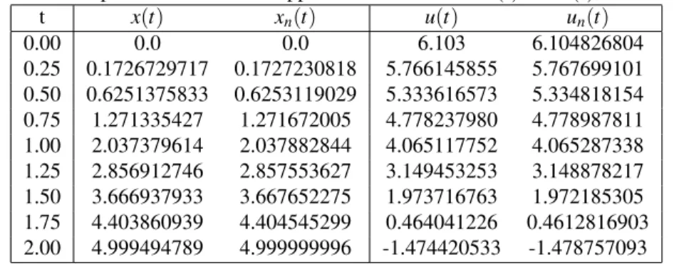
The accuracy of presented method is determined numerically for the absolute errors|x(t)−xn(t)|and|u(t)−xn(t)| as given in Table 4, for n=5.
Table 4: Comparison of exact and approximate solution ofx(t)andu(t); forn=5.
t x(t) xn(t) u(t) un(t)
0.00 0.0 0.0 6.103 6.104826804
0.25 0.1726729717 0.1727230818 5.766145855 5.767699101 0.50 0.6251375833 0.6253119029 5.333616573 5.334818154 0.75 1.271335427 1.271672005 4.778237980 4.778987811 1.00 2.037379614 2.037882844 4.065117752 4.065287338 1.25 2.856912746 2.857553627 3.149453253 3.148878217 1.50 3.666937933 3.667652275 1.973716763 1.972185305 1.75 4.403860939 4.404545299 0.464041226 0.4612816903 2.00 4.999494789 4.999999996 -1.474420533 -1.478757093
Note that, the previous problem is also solved by expanding x(t)into 7th order Boubaker series, and the founded optimal value is16.75072340, that is very close to both the exact value16.74543860and the result obtained in [27] (which is16.74531717for three iterations of their algorithms).
Example 5.3. (Controlled Linear and Duffing Oscillator [22, 26, 27])
Now we report the approximation of the state and control variables of the controlled linear oscillator problem with the following choice of the numerical values of the parameters in the standard case:
ω=1,T=2,x0=0.5,x0˙ =−0.5,
The object is to find the optimal control which minimizes
J=1 2
∫ 0 −2
u(t)2dt
, −2≤t≤0, (5.40)
when
u(t) =x¨(t) +x(t), (5.41)
and
x(−2) =0.5, x(0) =0, x˙(−2) =−0.5, x˙(0) =0. (5.42)
The approximation of x(.)is considered as follow:
x(t) =
3
∑
i=0
and then the control variable are obtained from the state equation (5.41), as follow:
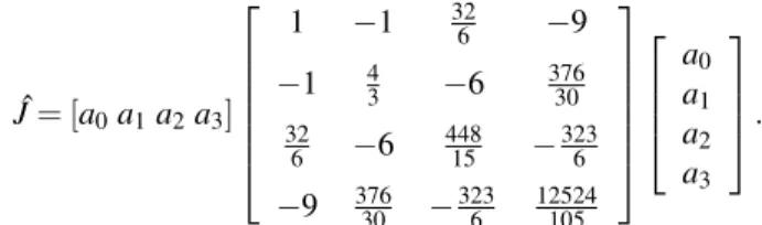
u(t) =4a2+7a3t+a0+a1t+a2t2+a3t3. (5.44) By substituting (5.44) into (5.40), the following expression forJ can be obtainedˆ
ˆ
J= [a0a1a2a3]
1 −1 326 −9
−1 43 −6 37630
32 6 −6
448
15 −
323 6
−9 37630 −323
6
12524 105
a0 a1 a2 a3
. (5.45)
From boundary conditions (5.42), another equations representing the initial states are obtained as follow:
a0−2a1+6a2−10a3= 1 2,
a0+2a2=0, (5.46)
a1−4a2+13a3=− 1 2, a1+a3=0.
The dynamic optimal control problem is approximated by a quadratic programming problem. The new problem is to minimize (5.45) subject to the equality constraint (5.46). The optimal value of the vectora∗ can be obtained from the standard quadratic programming method. By substituting these optimal parameters into (5.45), the approximate optimal value can be calculated. The optimal cost functional J, obtained by the presented method is shown for different n in Table 5.
Table 5: Optimal cost functionalJfor differentnin Example 5.3
n J Error
4 0.1849168913 5.8e−5 5 0.1848735296 1.5e−5 6 0.1848585740 3.2e−8
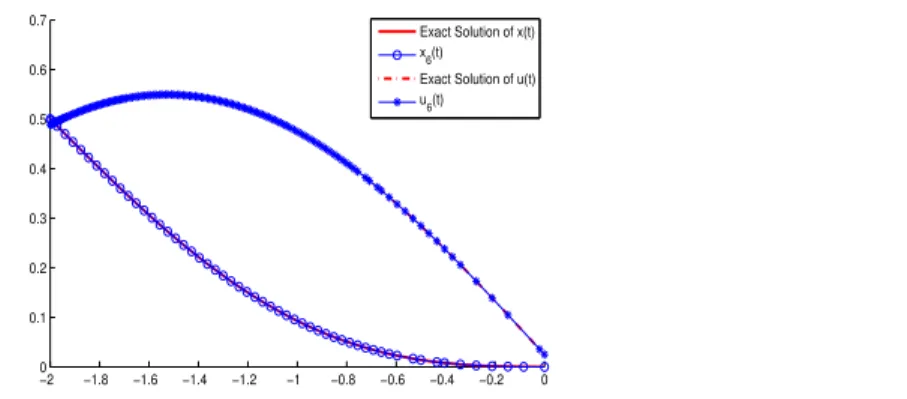
The exact solution for the performance index is J=0.1848585422. The optimal cost functional, J, obtained by the presented method for n=6is a very accurate approximation of the exact solution. This leads to state and control variables approximately as:
x(t) =0.0125t2−0.0895t3+0.00184t4+0.0127t5+0.00174t6
and
u(t) =0.0250−0.537t+0.0346t2+0.165t3+0.0540t4+0.0127t5+0.00174t6,
−2 −1.8 −1.6 −1.4 −1.2 −1 −0.8 −0.6 −0.4 −0.2 0 0
0.1 0.2 0.3 0.4 0.5 0.6 0.7
Exact Solution of x(t) x6(t) Exact Solution of u(t) u
6(t)
Figure 3: Solution of Example 5.3. The approximate solution forn=6 is compared with the actual analytical solution.
Also, the previous problem is solved by expanding x(t)into10thorder Boubaker series, and the optimal value is fond to be0.1848585424which is very close to the exact value0.1848585422. the result obtained in [26] and [27] are 0.184858576and0.184897926for three iterations of their algorithms. The maximum absolute error of state variable
(∥x(t)−xn(t)∥∞), control variable (∥u(t)−un(t)∥∞) and performance index (|J−Jn|) are listed in Table 6 for different n of presented algorithm.
Table 6: The maximum absolute error of state variable, control variable and performance index for differentn in Example 5.3
n ∥x(t)−xn(t)∥∞ ∥u(t)−un(t)∥∞ |J−Jˆ|
2 3.3e−2 1.1e−1 1.1e−2
3 3.2e−2 1.0e−1 1.0e−2 4 6.9e−4 7.7e−3 5.8e−5 5 3.0e−4 5.2e−3 1.5e−5
6 6.9e−6 1.9e−4 3.2e−8 7 1.1e−6 7.0e−5 2.3e−9 8 3.3e−8 2.2e−6 2.2e−10
9 2.6e−9 3.4e−7 2.1e−10 10 9.5e−10 8.5e−9 2.0e−10
The controlled Duffing Oscillator
Now, we investigate the optimal controlled Duffing oscillator. As mentioned before, the exact solution in this case is not known. Table 7 lists the optimal values of the cost functional J for various values ofεfor different n for controlled Duffing Oscillator.
Table 7: optimal cost functionalJfor Duffing oscillator problem for various values ofε. Present method
6 Conclusion
This paper presents a numerical technique for solving nonlinear optimal control problems and the controlled Duffing oscillator as a special class of optimal control problems. The solution is based on state parametrization. It produces an accurate approximation of the exact solution, by using a small number of unknown coefficients. We emphasize that this technique is effective for all classes of optimal control problems. In fact, the direct method proposed here has potential to calculating continuous control and state variables as functions of time. Also, the numerical value of the performance index is obtained readily. This method provides a simple way to adjust and obtain an optimal control which can easily be applied to complex problems as well. The convergence of the algorithms is proved. One of the advantages of this method is its fast convergence. Some illustrative examples are solved by this method, the results show that the presented method is a powerful method, which is an important factor to choose the method in engineering applications.
References
[1] A. E. Bryson, Y. C. Ho, Applied Optimal Control, Hemisphere Publishing Corporation, Washangton D.C, (1975).
[2] W. H. Fleming, C. J. Rishel, Deterministic and Stochastic Optimal Control, Springer-Verlag, New York, NY, (1975).
http://dx.doi.org/10.1007/978-1-4612-6380-7
[3] D. E. Kirk, Optimal Control Theory, an Introduction, Prentice-Hall, Englewood Cliffs, (1970).
[4] E. R. Pinch, Optimal Control and the Calculus of Variations, Oxford University Press, London, (1993).
[5] L. S. Pontryagin et al, The Mathematical Theory of Optimal Processes, In Interscience, John Wiley-Sons, (1962).
[6] J. E. Rubio, Control and Optimization: The Linear Treatment of Non-linear Problems, Manchester University Press, Manchester, (1986).
[7] S. A. Yousefi, M. Dehghan, A. Lotfi, Finding the optimal control of linear systems via He’s variational iteration method, Int. J. Comput. Math. 87 (5) (2010) 1042-1050.
http://dx.doi.org/10.1080/00207160903019480
[8] H. Saberi Nik, S. Effati, M. Shirazian, An approximate-analytical solution for the Hamilton-Jacobi-Bellman equa-tion via homotopy perturbaequa-tion method, Applied Mathematical Modelling, 36 (1) (2012) 5614-5623.
http://dx.doi.org/10.1016/j.apm.2012.01.013
[9] S. Effati, H. Saberi Nik, Solving a class of linear and nonlinear optimal control problems by homotopy perturba-tion method, IMA J Math. Control Info, 28 (4) (2011) 539-553.
[10] S. Berkani, F. Manseur, A. Maidi, Optimal control based on the variational iteration method, Computers and Mathematics with Applications, 64 (2012) 604-610.
http://dx.doi.org/10.1016/j.camwa.2011.12.066
[11] M. Keyanpour, M. Azizsefat, Numerical solution of optimal control problems by an iterative scheme, Advanced Modeling and Optimization, 13 (2011) 25-37.
[12] A. Jajarmi, N. Pariz, A. Vahidian, S. Effati, A novel modal series representation approach to solve a class of nonlinear optimal control problems, Int. J. Innovative Comput. Inform. Control, 7 (3) (2011) 1413-1425.
[13] B. Kafash, A. Delavarkhalafi, S. M. Karbassi, Application of variational iteration method for Hamilton-Jacobi-Bellman equations, Applied Mathematical Modelling, 37 (2013) 3917-3928.
http://dx.doi.org/10.1016/j.apm.2012.08.013
[15] O. Von Stryk, R. Bulirsch, Direct and indirect methods for trajectory optimization, Annal. Oper. Res, 27 (1992) 357-373.
http://dx.doi.org/10.1007/BF02071065
[16] I. Troch at el, Computing optimal controls for systems with state and control constraints, IFAC Control Appli-cations of Nonlinear Programming and Optimization, France, (1989) 39-44.
[17] H. M. Jaddu, Numerical Methods for solving optimal control problems using chebyshev polynomials, PhD thesis, School of Information Science, Japan Advanced Institute of Science and Technology, (1998).
[18] H. M. Jaddu, Direct solution of nonlinear optimal control problems using quasilinearization and Chebyshev polynomials, Journal of the Franklin Institute, 339 (2002) 479-498.
http://dx.doi.org/10.1016/S0016-0032(02)00028-5
[19] P. A. Frick, D. J. Stech, Solution of optimal control problems on a parallel machine using the Epsilon method, Optim. Control Appl. Methods, 16 (1995) 1-17.
[20] H. H. Mehne, A. H. Borzabadi, A numerical method for solving optimal control problems using state parametrization, Numer Algor., 42 (2006) 165-169.
http://dx.doi.org/10.1007/s11075-006-9035-5
[21] J. Vlassenbroeck, A chebyshev polynomial method for optimal control with state constraints, Automatica, 24 (4) (1988) 499-506.
http://dx.doi.org/10.1016/0005-1098(88)90094-5
[22] R. Van Dooren, J. Vlassenbroeck, A Chebyshev technique for solving nonlinear optimal control problems, IEEE Trans. Automat. Contr, 33 (4) (1988) 333-339.
http://dx.doi.org/10.1109/9.192187
[23] T. M. El-Gindy, H. M. El-Hawary, M. S. Salim, M. El-Kady, A Chebyshev approximation for solving opimal control problems, Comput. Math. Appl, 29 (1995) 35-45.
http://dx.doi.org/10.1016/0898-1221(95)00005-J
[24] G. N. Elnagar, M. Razzaghi, A Chebyshev spectral method for the solution of nonlinear optimal control prob-lems, Applied Mathematical Modelling, 21 (5) (1997) 255-260.
http://dx.doi.org/10.1016/S0307-904X(97)00013-9
[25] M. El-Kady, E. M. E. Elbarbary, A Chebyshev expansion method for solving nonlinear optimal control prob-lems, Applied Mathematics and Computation, 129 (2002) 171-182.
http://dx.doi.org/10.1016/S0096-3003(01)00104-7
[26] B. Kafash, A. Delavarkhalafi, S. M. Karbassi, Application of Chebyshev polynomials to derive efficient algo-rithms for the solution of optimal control problems, Scientia Iranica D, 19 (3) (2012) 795-805.
http://dx.doi.org/10.1016/j.scient.2011.06.012
[27] B. Kafash, A. Delavarkhalafi, S. M. Karbassi, Numerical Solution of Nonlinear Optimal Control Problems Based on State Parametrization, Iranian Journal of Science and Technology, 35 (A3) (2012) 331-340.
[28] K. P. Badakhshan, A. V. Kamyad, Numerical solution of nonlinear optimal control problems using nonlinear programming, Applied Mathematics and Computation, 187 (2007) 1511-1519
http://dx.doi.org/10.1016/j.amc.2006.09.074
[29] K. Boubaker, On Modified Boubaker Polynomials: Som Differential and Analytical Properties of the New Polynomials, Journal of Trends in Applied Science Research, 2 (6) (2007) 540-544.
[30] O. B. Awojoyogbe, K. Boubaker, A solution to Bloch NMR flow equations for the analysis of hemodynamic functions of blood flow system using m-Boubaker polynomials, International Journal of Current Applied Physics, 9 (1) (2009) 278-283.
http://dx.doi.org/10.1016/j.cap.2008.01.019
[31] M. Agida, A. S. Kumar, A Boubaker Polynomials Expansion Scheme Solution to Random Loves Equation in the Case of a Rational Kernel Electronic Journal of Theoretical Physics, International Journal of Current Applied Physics, 24 (2010) 319326.
[32] K. Boubaker, The Boubaker polynomials, a new function class for solving bi-varied second order differential equations, International Journal of Current Applied Physics, 25 (2009) 802-809.
[33] D. H. Zhang, Study of a non-linear mechanical system using Boubaker polynomials expansion scheme (BPES), International Journal of Non-Linear Mechanics, 46 (2011) 443-445.
http://dx.doi.org/10.1016/j.ijnonlinmec.2010.11.005
[34] A. Yildirim, S. T. Mohyud-Din, D. H. Zhang, Analytical solutions to the pulsed KleinGordon equation using modified variational iteration method (MVIM) and Boubaker polynomials expansion scheme (BPES), Comput. Math. Appl, 59 (2010) 2473-2477.
http://dx.doi.org/10.1016/j.camwa.2009.12.026