http://scma.maragheh.ac.ir
A SPECTRAL METHOD BASED ON THE SECOND KIND CHEBYSHEV POLYNOMIALS FOR SOLVING A
CLASS OF FRACTIONAL OPTIMAL CONTROL PROBLEMS
SOMAYEH NEMATI
Abstract. In this paper, we consider the second-kind Chebyshev polynomials (SKCPs) for the numerical solution of the fractional optimal control problems (FOCPs). Firstly, an introduction of the fractional calculus and properties of the shifted SKCPs are given and then operational matrix of fractional integration is introduced. Next, these properties are used together with the Legendre-Gauss quadrature formula to reduce the fractional optimal control prob-lem to solving a system of nonlinear algebraic equations that greatly simplifies the problem. Finally, some examples are included to con-firm the efficiency and accuracy of the proposed method.
1. Introduction
Fractional order dynamics have been received considerable recent at-tention and have been proved to model many real life problems such as, mechanical systems [11], solid mechanics [22], continuum and statisti-cal mechanics [21], fluid-dynamics [12], finance [15], viscoelastic dampers [17], viscoelasticity [4, 5], bioengineering [20], electromagnetic waves [13], control theory [7], etc.
FOCPs are one of the fractional dynamic systems that can be ap-peared in several problems in science and engineering. FOCP refers
2010Mathematics Subject Classification. 49J15, 26A33.
Key words and phrases. Fractional optimal control problems, Caputo fractional derivative, Riemann-Liouville fractional integral, Second-kind Chebyshev polynomi-als, Operational matrix.
to the minimization of an objective functional subject to dynamic con-straints, on state and control variables, which have fractional order mod-els. Although there are some different definitions of fractional deriva-tives, two types of them have been used very often for FOCP which are Riemann–Liouville and Caputo fractional derivatives. There are some numerical methods to solve FOCPs with these two types of definitions, for example see [1, 2, 3, 6, 14, 16, 18, 19, 26, 27, 28]. In the present pa-per, we consider the following optimal control problem with the Caputo fractional derivative [19]:
minJ = ∫ 1
0
f(t, x(t), u(t))dt, (1.1)
subject to:
Dtαx(t) =g(t, x(t)) +b(t)u(t), n−1< α≤n, b(t)̸= 0, (1.2)
D(i)x(0) =xi, i= 0,1, . . . , n−1,
(1.3)
where f and g are smooth functions of their arguments. The existence and uniqueness of the solution for the dynamical system (1.2) have been discussed in [10]. In this paper, we use the shifted second-kind Cheby-shev orthogonal basis for solving problem (1.1)–(1.3). To do this, we use operational matrix of fractional integration and Legendre-Gauss quad-rature formula. The main advantage of this method is that the problem is reduced to a system of algebraic equations. It can be seen that the operational matrix of fractional integration for Chebyshev basis needs much fewer computational efforts compared with that for Legendre ba-sis introduced in [19] (see Section 2) and it makes our method more computationally attractive.
The structure of this paper is arranged in the following way: In Sec-tion 2, an introducSec-tion of fracSec-tional calculus and properties of the shifted SKCPs are given and also, the operational matrix of fractional integra-tion is introduced. In Secintegra-tion 3, a numerical method is considered to solve problem (1.1)–(1.3). In Section 4, illustrative examples are in-cluded to demonstrate the applicability and efficiency of the method. Finally, a brief conclusion is given in Section 5.
2. Preliminaries and notations
Definition 2.1. The fractional derivative ofx(t) in the Caputo sense is defined as follows
Dtαx(t) =
1 Γ(n−α)
∫t
0(t−τ)n−α−1
dn
dτnx(τ)dτ, n−1< α < n,
x(n)(t) α=n,
where nis the ceiling function ofα and
Γ(α) = ∫ ∞
0
tα−1e−tdt.
Definition 2.2. The Riemann-Liouville fractional integral operatorIα t
of order α is given by
Itαx(t) =
1 Γ(α)
∫t
0(t−τ)α−1x(τ)dτ, α >0,
x(t), α= 0.
Some properties of the Riemann-Liouville fractional integral operator Iα
t and the Caputo fractional differential operatorDαt are as follows:
(2.1) Itαtk= Γ(k+ 1) Γ(k+ 1 +α)t
k+α, α
≥0, k >−1,
DαtItαx(t) =x(t),
(2.2) ItαDαtx(t) =x(t)−
n−1 ∑
i=0
x(i)(0)t
i
i!, n−1< α≤n, t >0.
Definition 2.3. The shifted SKCP of orderiis defined on [0,1] as
ψi(t) =Ui(2t−1), i= 0,1,2, . . . ,
whereUi(t) is the well-known SKCP of orderi. We note that the SKCPs
are orthogonal functions on the interval [−1,1] and can be determined with the aid of the following recursive formula:
Ui(t) = 2tUi−1(t)−Ui−2(t), i≥2, with U0(t) = 0 and U1(t) = 2t.
The orthogonal property for the shifted SKCPs is as follows:
∫ 1 0
w(t)ψi(t)ψj(t)dt=
{ π
4, i=j, 0, otherwise,
where w(t) =√4t−4t2.
The shifted SKCP of ordericould be written as:
(2.3) ψi(t) =
i
∑
k=0
(−1)i−k (i+k+ 1)!22k
(i−k)!(2k+ 1)!t
A functionx(t), square integrable on [0,1], can be expanded using the shifted SKCPs as follows:
(2.4) x(t)≃
∞
∑
i=0
ciψi(t),
where
(2.5) ci =
4 π
∫ 1 0
w(t)x(t)ψi(t)dt, i= 0,1,2, . . . .
If we consider the first N + 1 terms in (2.4), an approximation of the functionx(t) is obtained as:
x(t)≃
N
∑
i=0
ciψi(t) =CTψ(t),
in which
C= [c0, c1, . . . , cN]T,
and
ψ(t) = [ψ0(t), ψ1(t), . . . , ψN(t)]T.
(2.6)
Considering the vectorψ(t) in equation (2.6), we get the following result:
Theorem 2.4. If ψ(t)is the shifted SKCPs vector defined by (2.6), then the fractional Integral of order α of this vector is given by
(2.7) Itαψ(t)≃P(α)ψ(t),
where P(α) is the (N + 1)×(N + 1) operational matrix of fractional
Integration as
P(α) =
θα(0,0) θα(0,1) . . . θα(0, N)
θα(1,0) θα(1,1) . .. θα(1, N)
..
. ... . .. ...
θα(N,0) θα(N,1) . . . θα(N, N)
,
in which n is the ceiling function ofα and
(2.8)
θα(i, j) = i
∑
k=0
(−1)i−k(j+ 1)22(k+1)k!(i+k+ 1)!Γ(
k+α+32)
√
Proof. Using equations (2.1) and (2.3), for i= 0,1, . . . , N we have
Itαψi(t) = i
∑
k=0
(−1)i−k (i+k+ 1)!22k
(i−k)!(2k+ 1)!I
α ttk
=
i
∑
k=0
(−1)i−k (i+k+ 1)!22kk!
(i−k)!(2k+ 1)!Γ(k+α+ 1)t
k+α.
(2.9)
Approximatingtk+αusing the shifted second-kind Chebyshev series gives
(2.10) tk+α=
N
∑
j=0
akjψj(t),
where akj are obtained from (2.5) as follows
akj =
4(j+ 1)Γ(k+α+32)Γ(k+α+ 1)
√
πΓ(k+α+j+ 3)Γ(k+α−j+ 1), j= 0,1,2, . . . , N.
Substituting (2.10) into equation (2.9), we have
Itαψi(t) = N
∑
j=0
θα(i, j)ψj(t),
whereθα(i, j) is defined by (2.8). Therefore, fori= 0,1, . . . , N we obtain
(2.11) Itαψi(t) = [θα(i,0), θα(i,1), . . . , θα(i, N)]ψ(t).
Finally, equation (2.7) is established using equation (2.11). □
3. Numerical method
In this section, we present a numerical method to solve FOCP (1.1)– (1.3) using properties of the shifted SKCPs . To do this, we consider an approximation of the fractional state rate Dα
tx(t) in the dynamical
system (1.2) as:
(3.1) Dαtx(t)≃
N
∑
i=0
ciψi(t) =CTψ(t),
where the elements ci of the vector C are unknown and ψ(t) is given
by (2.6). Considering equations (1.3), (2.2) and (3.1) and using the operational matrix of fractional integration in equation (2.7), we have
(3.2) x(t)≃CTP(α)ψ(t) +
n−1 ∑
i=0 xi
ti
Now, we can approximate u(t) using the dynamical system in equation (1.2) as:
(3.3) u(t)≃ 1 b(t)
[
CTψ(t)−g (
t, CTP(α)ψ(t) +
n−1 ∑ i=0 xi ti i! )] .
Substituting (3.2) and (3.3) into (1.1), we obtain
J[C] = ∫ 1
0 f
(
t, CTP(α)ψ(t) +
n−1 ∑ i=0 xi ti i!, 1 b(t) [
CTψ(t)−g (
t, CTP(α)ψ(t) +
n−1 ∑ i=0 xi ti i! )]) dt. (3.4)
Let us introduce
Q(C, t) =f (
t, CTP(α)ψ(t) +
n−1 ∑ i=0 xi ti i!, 1 b(t) [
CTψ(t)−g (
t, CTP(α)ψ(t) +
n−1
∑ i=0 xi ti i! )]) dt.
So, using Legendre-Gauss quadrature formula we have
J[C]≃ 1
2
m
∑
k=1 wkQ
( sk+ 1
2 , C )
,
where sk,k= 1,2, . . . , mare mzeros of Legendre polynomial of degree m and wk are the corresponding weights [9]. Finally, the necessary
conditions for the optimality of the performance index imply:
(3.5) ∂J
∂cj
[C] = 0, j= 0,1, . . . , N.
Equation (3.5) forms a nonlinear system of algebraic equations in terms of the unknown elements of the vector C. In our implementation, we have solved this system using the Mathematica function FindRoot, which uses the Newton’s method as the default method. After solving this system the numerical results forx(t),u(t) and optimum value of J are given using equations (3.2), (3.3) and (3.4), respectively.
4. Numerical examples
Example 4.1. Consider a minimization problem as follows [19]:
minJ = ∫ 1
0
(
x(t)−t2)2+ (
u(t) +t4− 20t
9 10
9Γ(109 ) )2
dt,
subject to:
D1t.1x(t) =t2x(t) +u(t),
x(0) =x′(0) = 0.
The functions x(t) = t2 and u(t) = −t4+ 20t
9 10
9Γ(9 10)
minimize the per-formance index J and the minimum value is J = 0. We have solved this problem with different values for N. For instance, withN = 3 the operational matrix of fractional integration is obtained as:
P(1.1) =
0.452542 0.242828 0.00714199 −0.00140498
−0.35846 −0.0354935 0.107481 0.00509663 0.166877 −0.0600908 −0.0166159 0.0679421
−0.120681 −0.00390251 −0.0478958 −0.0109875
,
and the unknown vector C is calculated by solving the final system in equation (3.5) with initial approximation C= [0,0,0,0]T as:
C=
1.09993 0.507813
−0.0163147 0.0042012
.
Numerical results for the minimum of J with different values of N to-gether with the results obtained in [19] using Legendre functions are shown in Table 1.
Table 1. Numerical results for Example 4.1
Present method Method of [19]
N J m J
3 5.82938×10⁻⁶ 3 6.0753×10⁻⁶
4 1.46226×10⁻⁶ 4 1.67255×10⁻⁶
5 4.3337×10⁻⁷ 5 5.91532×10⁻⁷
7 3.5498×10⁻⁸ 7 1.21966×10⁻⁷
Example 4.2. Consider the following minimization problem [19]
minJ = ∫ 1
0 [
et(
x(t)−t4+t−1)2
+(t2+ 1) (
u(t) + 1−t+t4− 8000t
21 10
77Γ(1 10
) )2
dt,
subject to:
Dt1.9x(t) =x(t) +u(t),
x(0) = 1, x′(0) =−1.
In this problem the performance index J takes its minimum value when x(t) = 1−t+t4 and the minimum value is J = 0. By choosing N = 3, the operational matrix of fractional integration is as follows:
P(1.9) =
0.178143 0.138152 0.031611 −0.00061084
−0.18579 −0.108697 0.00600659 0.0117374 0.113265 0.0388703 −0.0197332 0.00231601
−0.0726456 −0.0254721 −0.000646971 −0.0104707
,
and the unknown vector C is obtained with initial approximation C = [0,0,0,0]T as:
C=
3.27996 2.70114 0.728038 0.0128955
.
Table 2 presents the numerical results for the minimum of performance indexJ with different values ofN obtained by the presented method in this paper and the results obtained in [19] using Legendre functions.
Table 2. Numerical results for Example 4.2
Present method Method of [19]
N J m J
3 1.16577×10⁻⁴ 3 8.93768×10⁻⁶
4 5.32891×10⁻⁷ 4 5.42028×10⁻⁷
5 6.50811×10⁻⁸ 5 6.77757×10⁻⁸
7 1.94565×10⁻⁹ 7 2.84624×10⁻⁹
Example 4.3. Consider the following minimization problem [19]
minJ = ∫ 1
0 [
x2(t)−2t32x(t) +u2(t)−3
√
π 4 e
−tu(t) +e−t+t 3 2
u(t)
+t3+9π 64e
−2t
−3 √
π 8 e
−2t+t 3 2
+1 4e
−2t+2t 3 2
+e2t ]
dt,
subject to:
D1t.5x(t) =ex(t)+ 2etu(t), x(0) =x′(0) = 0.
In this example the state functionx(t) =√t3and the control function u(t) = 12e−t
(
−et 3 2
+ 3√4π )
minimize the performance index J and the
minimum value is J = 3.19452805. We applied the proposed method in this paper withN = 2 such that for this choice we have
P(1.5)=
0.2919 0.1946 0.0265364
−0.27244 −0.106146 0.0449077 0.147846 0.00898155 −0.0336128
,
and the unknown vector C is obtained with initial approximation C = [0,0,0]T as:
C= 1.32797 0.00085962 −0.00105561 .
Finally, the performance index with N = 2 is gained J = 3.19455842. Also, Table 3 gives the numerical results for the minimum of performance indexJ with different values of N.
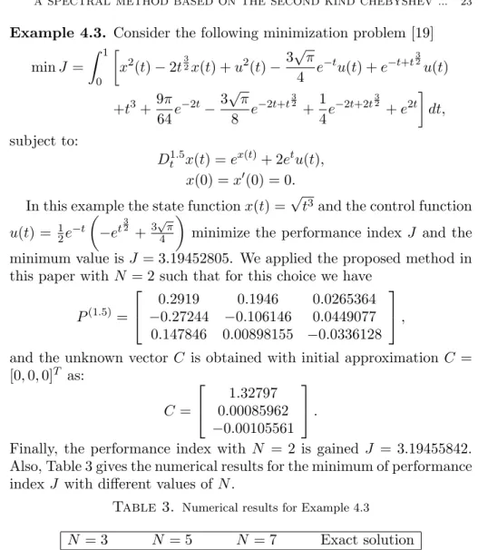
Table 3. Numerical results for Example 4.3
N = 3 N = 5 N = 7 Exact solution
3.19453043 3.19452812 3.19452805 3.19452805
Example 4.4. As the final example, consider the following problem [19]:
minJ = 1 2
∫ 1 0
[
x2(t) +u2(t)] dt,
subject to:
The exact solution of this problem withα= 1 was given by [8] as:
x(t) =βsinh(√2t)+ cosh(√2t),
u(t) =(β+√2)sinh(√2t)+(√2β+ 1)cosh(√2t),
where
β =−
√
2 sinh(√ 2)
+ cosh(√ 2) sinh(√
2)
+√2 cosh(√ 2).
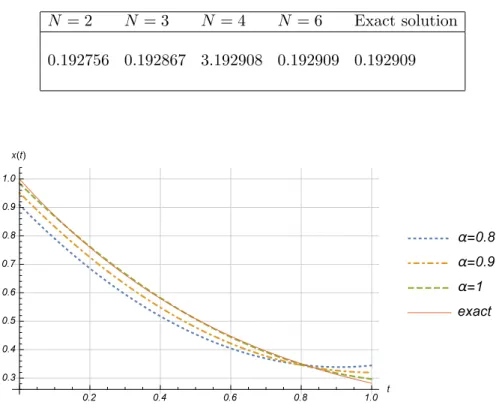
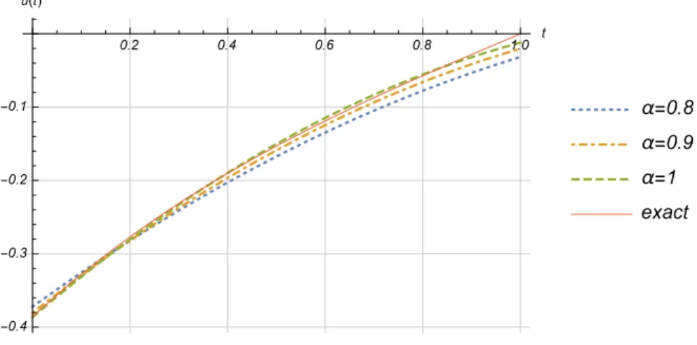
Numerical results for this problem are shown in Table 4 and Figures 1 and 2. In Table 4, minimum value for J when α = 1 is presented with different values of N and Figures 1 and 2 display the approximate solutions for x(t) and u(t), respectively, with α= 0.8,0.9,1 and N = 2 together with their exact solutions.
Table 4. Numerical results for Example 4.4
N = 2 N = 3 N = 4 N = 6 Exact solution
0.192756 0.192867 3.192908 0.192909 0.192909
Figure 2. Comparison ofu(t) withN= 2 for Example 4.4
5. Conclusions
In this paper, a numerical method has been proposed for numerical solution of the FOCPs. By using the definition of Riemann-Liouville fractional integral operator and properties of the shifted SKCPs, the operational matrix of fractional integration has been introduced. This matrix and Legendre-Gauss quadrature formula have been employed to reduce the considered problem into a system of nonlinear algebraic equations. The method was tested on some examples and the numerical results obtained by the proposed method in this paper have been com-pared with the results achieved using the numerical technique discussed in [19]. Also, the results approved that the proposed method is efficient and has high accuracy.
References
1. O.M.P. Agrawal, A general formulation and solution scheme for fractional op-timal control problem, Nonlinear Dynam., 38 (2004) 323–337.
2. O.M.P. Agrawal,A Hamiltonian formulation and a direct numerical scheme for fractional optimal control problems, J. Vib. Control, (2007) 1269–1281.
3. O.M.P. Agrawal, A formulation and numerical scheme for fractional optimal control problems, J. Vib. Control, 14 (2008) 1291–1299.
4. R.L. Bagley and P.J. Torvik,A theoretical basis for the application of fractional calculus to viscoelasticity, J. Rheol., 27 (1983) 201–210.
5. R.L. Bagley and P.J. Torvik, Fractional calculus in the transient analysis of viscoelastically damped structures, AIAA J., 23 (1985) 918–925.
7. G. Bohannan,Analog fractional order controller in temperature and motor con-trol applications, J. Vibr. Concon-trol, 14 (2008) 1487–1498.
8. K.B. Datta and B.M. Mohan, Orthogonal Functions in Systems and Control, World Scientific, Singapore, 1995.
9. R.A. Devore and L.R. Scott,Error bounds for Gaussian quadrature and
weighted-L1
polynomial approximation, SIAM J. Numer. Anal., 21 (1984) 400–412. 10. K. Diethelm and N.J. Ford, Multi-order fractional differential equations and
their numerical solution, Appl. Math. Comput., 154 (2004) 621–640.
11. W. Grzesikiewicz, A. Wakulicz, and A. Zbiciak,Non-linear problems of fractional in modelling of mechanical systems, Int. J. Mech. Sci., 70 (2013) 90–89. 12. J.H. He, Some applications of nonlinear fractional differential equations and
their applications, Bull. Sci. Technol., 15 (1999) 86–90.
13. M. Ichise,Y. Nagayanagi, and T. Kojima, An analog simulation of noninteger order transfer functions for analysis of electrode process, J. Electroanal. Chem., 33 (1971) 253–265.
14. H. Jafari, and H. Tajadodi, Fractional order optimal control problems via the operational matrices of Bernstein polynomials, U.P.B. Sci. Bull., Series A, 76(3) (2014) 115–128.
15. Y. Jiang, X. Wang, and Y. Wang,On a stochastic heat equation with first order fractional noises and applications to finance, J. Math. Anal, Appl., 396 (2012) 656–669.
16. E. Keshavarz, Y. Ordokhani, and M. Razzaghi, A numerical solution for frac-tional optimal control problems via Bernoulli polynomials, J. Vib. Control, 29 (2015) 1–15.
17. R. Lewandowski, and B. Chorazyczewski,Identification of the parameters of the Kelvin-Voigt and the Maxwell fractional models, used to modeling of viscoelastic dampers, Comput. Struct., 88 (2010) 1–17.
18. A. Lotfi, M. Dehghan, and S.A. Yousefi,A numerical technique for solving frac-tional optimal control problems, Comput. Math. Appl., 62 (2011) 1055–1067. 19. A. Lotfi, S.A. Yousefi, and Mehdi Dehghanb, Numerical solution of a class of
fractional optimal control problems via the Legendre orthonormal basis combined with the operational matrix and the Gauss quadrature rule, J. Comput. Appl. Math., 250 (2013) 143–160
20. R.L. Magin,Fractional calculus in bioengineering, Crit. Rev. Biomed. Eng., 32 (2004) 1–104.
21. F. Mainardi,Fractional calculus: some basic problems in continuum and statis-tical mechanics, Fract. Fract. Calculus Contin. Mech., 387 (1997) 291–348. 22. Y.A. Rossikhin and M.V. Shitikova, Applications of fractional calculus to
dy-namic problems of linear and nonlinear hereditary mechanics of solids, Appl. Mech. Rev., 50 (1997) 15–67.
23. N. Sebaa, Z.E.A. Fellah, W. Lauriks, and C. Depollier,Application of fractional calculus to ultrasonic wave propagation in human cancellous bone, Signal Pro-cess., 86 (2006) 2668–2677.
24. V.E. Tarasov,Fractional vector calculus and fractional Maxwells equations, An-nals of Physics, 323 (2008) 2756–2778.
25. J.A. Tenreiro Machado, P. Stefanescu, O. Tintareanu, and D. Baleanu, Frac-tional calculus analysis of the cosmic microwave background, Rom. Rep. Phys., 65 (2013) 316–323.
27. C. Tricaud and Y.Q. Chen, An approximation method for numerically solving fractional order optimal control problems of general form, Comput. Math. Appl., 59 (2010) 1644–1655.
28. S.A. Yousefi, A. Lotfi, and M. Dehghan, The use of a Legendre multiwavelet collocation method for solving the fractional optimal control problems, J. Vib. Control, 13 (2011) 1–7.
29. S.B. Yuste, L. Acedo, and K. Lindenberg, Reaction front in an A+B −→ C
reaction-subdiffusion process, Phys. Rev. E., 69(2004) 036126.
Department of Mathematics, Faculty of Mathematical Sciences, Uni-versity of Mazandaran, Babolsar, Iran.
![Table 2 presents the numerical results for the minimum of performance index J with different values of N obtained by the presented method in this paper and the results obtained in [19] using Legendre functions.](https://thumb-eu.123doks.com/thumbv2/123dok_br/18147393.327167/8.918.215.681.170.410/presents-numerical-performance-different-presented-obtained-legendre-functions.webp)