Comparison to Ordinary PLS-DA
Anna Telaar1, Kristian Hovde Liland2, Dirk Repsilber1, Gerd Nu¨rnberg1*
1Institute for Genetics and Biometry, Department of Bioinformatics and Biomathematics, Leibniz Institute for Farm Animal Biology, Dummerstorf, Germany,2Department of Chemistry, Biotechnology and Food Science, Norwegian University of Life Sciences, A˚s, Norway
Abstract
Classification studies are widely applied, e.g. in biomedical research to classify objects/patients into predefined groups. The goal is to find a classification function/rule which assigns each object/patient to a unique group with the greatest possible accuracy (classification error). Especially in gene expression experiments often a lot of variables (genes) are measured for only few objects/patients. A suitable approach is the well-known method PLS-DA, which searches for a transformation to a lower dimensional space. Resulting new components are linear combinations of the original variables. An advancement of PLS-DA leads to PPLS-DA, introducing a so called ‘power parameter’, which is maximized towards the correlation between the components and the group-membership. We introduce an extension of PPLS-DA for optimizing this power parameter towards the final aim, namely towards a minimal classification error. We compare this new extension with the original PPLS-DA and also with the ordinary PLS-DA using simulated and experimental datasets. For the investigated data sets with weak linear dependency between features/variables, no improvement is shown for PPLS-DA and for the extensions compared to PLS-DA. A very weak linear dependency, a low proportion of differentially expressed genes for simulated data, does not lead to an improvement of PPLS-DA over PLS-DA, but our extension shows a lower prediction error. On the contrary, for the data set with strong between-feature collinearity and a low proportion of differentially expressed genes and a large total number of genes, the prediction error of PPLS-DA and the extensions is clearly lower than for PLS-DA. Moreover we compare these prediction results with results of support vector machines with linear kernel and linear discriminant analysis.
Citation:Telaar A, Liland KH, Repsilber D, Nu¨rnberg G (2013) An Extension of PPLS-DA for Classification and Comparison to Ordinary PLS-DA. PLoS ONE 8(2): e55267. doi:10.1371/journal.pone.0055267
Editor:Kewei Chen, Banner Alzheimer’s Institute, United States of America
ReceivedJanuary 17, 2012;AcceptedDecember 27, 2012;PublishedFebruary 11, 2013
Copyright:ß2013 Telaar et al. This is an open-access article distributed under the terms of the Creative Commons Attribution License, which permits unrestricted use, distribution, and reproduction in any medium, provided the original author and source are credited.
Funding:The study was supported by the Max Planck Institute for Infection Biology, Berlin, and the German Federal Minstry of Education and Research. The funders had no role in study design, data collection and analysis, decision to publish, or preparation of the manuscript.
Competing Interests:The authors have declared that no competing interests exist. * E-mail: [email protected]
Introduction
In discrimination studies, data sets are often handled having high numbers of features but only few samples. Especially for gene expression experiments, where thousands of genes are measured and in comparison only few samples are used, dimension reduction is advantageous as a pre-processing step before the final classification step takes place. There exist a lot of feature extraction methods for dimension reduction. One such method is powered partial least squares discriminant analysis (PPLS-DA) which is a specialized version of the well-known partial least squares discriminant analysis (PLS-DA), which was first intro-duced in chemometrics by Wold et al. [1] by using the PLS regression [2] for classification purposes. Here the response variable (Y) in the linear model is given in form of indicator variables. Barker & Rayens [3] and Nocairi et al. [4] were the first to formulate PLS-DA accurately. The aim is to reduce the dimensions (number of features) by coordinate transformation to a lower dimensional space. PPLS-DA was introduced by Liland and Indahl in [5] to improve the calculation of the loading weights for better separation of the groups by introducing a power parameter analogously to powered partial least squares (PPLS) [6] and maximizing the correlation between the data matrix and the group memberships, analogous to Fisher’s canonical discriminant
anal-ysis (FCDA). The optimization criterion in PPLS-DA is therewith not directly aimed at prediction, and therefore the original algorithm does not necessarily yield the best components for class prediction.
Materials and Methods
Description of a Classification Problem
Ann|pdata matrixXwithnobjects andpfeatures together with a vectory~(y1,. . .,yn)tof group memberships form the basis of a classification problem. Here yi[G,i~1,. . .,nis the group label for objectiwhich for example can be given in the form of discrete variables or symbolics. The k-th column of the matrixXis denoted byxk. We assume that each sample belongs to a unique
group g and each group has a sample size of ng and a prior probability of group membership ofpg. In totalGdifferent groups exist andn~PGg~1 ng. In this article, we restrict ourselves to only two different groupsG~2. Our results can be extended to more than two groups.
The group information can also be given in the form of a dummy coded matrixYas followsY~(yig)i~1,...,n,g~1,2,yigequals 1 if sample ibelongs to groupsg, otherwise the entry equals 0,
i~1,. . .,n and g~1,2. The goal is to determine a function
C:Rp?G which assigns to each object a unique group (x.y) with the greatest possible accuracy [8]. In the following we assume that X is centered. Therewith the empirical total covariance matrixTis equal toXtX, and letBdenote the empirical between group sum of squares and cross-product matrix, which can be formalized asB~XtSXwithS~Y(YtY){1Yt[8].
Introduction of PLS-DA and PPLS
PLS-DA. Before we start with the detailed description of PPLS-DA, we give a brief introduction to the roots of this method, PLS-DA and PPLS. Leta[Rpbe a vector of loadings withata~1 and t[Rp a vector containing the mean values of the groups, t~XtY(YtY){1
. Nocairi et al. [4] showed that the dominant eigenvector ofBmaximized the covariance betweenXaandtin the context of classification. Therefore this eigenvector should be used for the determination of the loading weights vector which was also recommended by Barker & Rayens [3]. An enhanced version of PLS-DA with inclusion of prior probabilities (pg) in the estimation ofBis proposed by Indahl et al. [8]. In this version, the importance of each group no longer depends on the empirical prior probabilities. Therewith a direct opportunity is given to put more weight on special groups for the calculation of the loading weights. MoreoverXis transformed to ann|2matrixZ~XW0, here W0~XtY
ffiffiffiffi P p
(YtY){1 and P~diag(fp
gDg~1,2g). There-with aG|Geigenvalue problem (B[Rp|p) is reduced to a2|2 eigenvalue problem (2 = number of groups), because only the between-group covariance matrix according to Zis considered (BP~nZtY(YtY)
{1P(YtY){1YtZ). Afterwards the eigenvalue
needs to be back transformed byW0.
PPLS. Now we are turning back to PLS regression, to explain the introduction of the power parametercin PLS regression. The
loading weights vector of PLS regressionw~½w1,. . .,wp~ Xty DDXtyDD maximizescov(Xw,y)and can be rewritten as.
w~k:½cov(y,x1),. . .,cov(y,xp)t
~k:sd(y)½corr(y,x1):sd(x1),. . .,corr(y,xp):sd(xp)t,
with a scaling constant k where cov, corr and sd denote covariance, correlation and standard deviation, respectively. Hence, the influence on the loading weights of the correlation and standard deviation part is balanced. DominatingX-variance which is irrelevant for prediction does not lead to optimal models, therefore Indahl et al. [6] propose PPLS which allows the user to
control the importance of the correlation part and the standard deviation part by a power parametercas follows:
w(c)~k(c): s1:Dcorr(x1,y)D c 1{c:sd(x
1) 1{c
c . . .,s
p:Dcorr(xp,y)D c 1{c:sd(xp)1
{c c
t
:
Here sj denotes the sign ofcorr(xj,yg). The power parameter
c[½0,1 is determined such that the correlation is maximal:
arg max
c[(0,1)corr(Xw(c),y). Alsoc equal to 0 and 1 is included in the maximization problem by calculation correlation with a loading weights vector which has only a non-zero entry (forc~0) for the feature with the largest standard deviation and by determining the correlation according to a loading weights vector which has only a non-zero entry for the feature with the largest correlation toy(c~1).
PPLS-DA: Optimization of the Power Parameter According to Correlation
PPLS-DA is designed to deliver components which are optimal for discriminating the cases coded inY. This optimality can be understood in terms of a correlation approach. Nocairi et al. showed in [4], that correlation is determined by the so called Rayleigh quotient.
r2(Xa,t)~a tBa
atTa: ð1Þ
Here the correlation is measured by the squared coefficient of correlation r2. Maximization of the correlation is therewith equivalent to maximization of the Rayleigh quotient.
arg max a[Rp
atBa
atTa: ð2Þ
The well known solution of the maximization problem (2) is the dominant eigenvectoramaxofT{1B. This is exactly the approach of Fishers`s canonical discriminant analysis (FCDA) for determin-ing the vector of loaddetermin-ings.
For PPLS-DA, Liland and Indahl combine in [5] the approaches of FCDA and PPLS and further include, like in [8], prior probabilitiespgfor each groupgin the calculation ofTand B. The data matrix Xis transformed with W0(g) to then|G matrix Z(c)~XW0(c), where W0(c) contains the possible candidate loading weights vectors as columns.
wg(c)~Kg,c:vg,c, ð3Þ
with
vg,c~ s1:Dcorr(x1,yg)D
c
1{c(x
1) 1{c
c . . .,s
p:Dcorr(xp,yg)D
c
1{c(x
p)
1{c c
h it
,
Kg~nsd(y):pffiffiffiffiffipg=ng,g~1,. . .,Gandc[(0,1).
matrix is obtained as TP(c)~nZ(c)tVPZ(c) with
P~diag(fp1,p2g) and VP~diag(fviDvi~npg=ng,i~1,. . .,ng) [5]. VP is an n|n diagonal matrix where the non-zero entry belonging to sampleiis the ratio of the prior probability of the group to whichibelongs and the corresponding group size times the number of samplesn.
The maximization problem of PPLS-DA is as follows.
arg max
c[½0,1
atB
P(c)a
atT
P(c)a
: ð4Þ
Forc~0the feature(s) with the highest standard deviation are tested and forc~1the feature(s) with the highest correlation to the group membership vector are checked separately. We denote the solution of the optimization problem (4) bycmax. To avoid singular matrices TP(c) and to get a numerically more stable solution, Liland and Indahl [5] substitute the maximization problem (4) by the maximization problem argmax
c[½0,1cca(Z(c),Y), where cca
denotes the canonical correlation. In [9] the authors showed that these procedures lead to equal results.
For each component,cmaxis determined by maximization of the canonical correlation:
cmax~argmax
c[½0,1cca(Z(c),Y): ð5Þ
In the algorithm of PPLS-DA in the R package pls, the R function optimize is used to search for the maximum. For this purpose, the whole training set is used to findcmax. Transforming X into an n|g data matrix Z(c), the maximization problem depends on the number of groups and number of samples. It does not depend on the usually much higher number of features. The final loading weight vector is then w~W0(cmax)acmax. For a
detailed description of PPLS-DA we refer to [5].
In our experience with PPLS-DA, we have observed that optimization ofcmax does not always lead to the lowest possible prediction error available through other choices ofc.
PPLS-DA: Optimizing the Power Parametercwith Respect to Prediction
To improve prediction errors in classification tasks using PPLS-DA, we aim at optimizing the power parametercwith respect to prediction error of LDA. For this, we propose a cross-validation approach, to avoid overfitting. Therefore, we separate in a first step the data into a training and a test set which are disjunct. We now call these sets outer training set and outer test set. Using only the outer training set to optimize thec{value, we use the outer test set to evaluate the computed classification function. In a next step we split the outer training set randomly in Ninner different inner training and inner test sets. Because unbalanced data have influence on the estimated classifier, we down-sample the majority group objects to get equal numbers of objects in both groups for the outer training set. Here, the proportion of 0.7 of the smallest group size determines the size of the outer training set for each group. The remaining objects build the outer test set. For the optimization step, we take into account equidistant fixedc{values in [0,1] with step sizenc, resulting in a sequence ofc{values for
the optimizationc1~0,c2,. . .,c1
ncz1
~1. For example for a choice
ofnc~0:1, we consider 11c{values,0,0:1,0:2. . .,0:9,1.
We calculate the prediction error (PE), the proportion of wrongly classified samples of a test set, as a measure for good classification. In Figure 1 a rough overview of our proposed extension is given. In this paper, all cross-validation procedures consist of random samples of the corresponding data sets to the proportions of 0.7 (training set) and 0.3 (test set). For example, a cross-validation with 10 repeats, repeats the sampling 10 times. Utilizing the statistical software R, we use the function cppls (of the package pls) for PPLS-DA and the function lda (of the R-package MASS). Furthermore, we use the default setting for the priors in the lda function, using the proportions of the groups which are equal in our cases.
We propose an extension for optimizing both,cand the number of components to be used as input for the LDA. The optimization of thec-value depends on the parametersNinnerandnc.
In our extension all components are used to optimize the c{value minimizing PE. The number of components and the power parameter are optimized in one procedure. Therewith all components have the samec{value.
In the optimization, for each fixedc{value (ci,i~1. . .,1
nc
z1)
the optimal number of components of PPLS-DA is determined as follows (see Figure 2): For theNinnerdifferent inner test sets, the PE for one up to five components Cj, j~1,. . .,5 is calculated, all using the same ci resulting in a matrix (PEs,Cj)s,j,
s~1,. . .Ninner,j~1,. . .,5. Then the average inner PE is calcu-lated for each component. Therewith we select for each ci the smallest mean PE over the Ninner-test sets with a corresponding optimal number of components (ci). We search for the minimal PE leading tocoptwith the optimal number of componentscopt. For thesecoptcomponents and the power parametercopt, we calculate the corresponding loading weights vectors on the outer training set, and we finally determine the PE of the outer test set.
R Functions Used
(P)PLS-DA implementations. For PPLS-DA, we used the function cppls of the package pls. We implemented an R-code for PLS-DA based on [8]. The optimal number of components was determined by a cross-validation on the outer training set for PLS-DA, PPLS-DA withcmax and our described extensions of PPLS-DA. For this step, we restricted the maximal number of components to five. The segments of the cross-validation are randomly chosen at the proportion of 0.7 and 0.3 of the data set. We repeat this procedure 10 times.
Further Classification Methods
SVM. The classification method SVM with a linear kernel searching for a linear hyperplane for the separation of the data is considered for comparison. For this purpose the R package e1071 [10] is applied and the parameterCfor the linear kernel is tuned within the interval½2{5,24using the R-function tune.svm with a cross-validation of 10 steps. The interval for tuning is chosen according to the suggestion of Dettling & Buehlmann [11].
t-LDA. Additionally an LDA is performed using ten features which are filtered based on the outer training set according to a ranking list based on the lowest p-value of the t-test. For the t-test we use the R-package stats.
The same segments of the outer training and outer test set are used across all tested methods for fair comparison.
Data
data are on the log-scale of gene expression as for the simulated data.
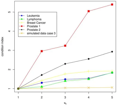
For detailed description of the covariance structure of our data, we use two measures analogous to Sæbø et al. in [12]. The condition index, first used in [13], and the absolute value of the covariances between the principal components of X and the response vector as used in [12]. The condition indexkj~ ffiffiffiffiffiffiffiffiffiffiffil1=lj
p ,
j~1,. . .,pis used as a measure for variable dependence, withlk being the kth eigenvalue of cov(X). It can be assumed that l1§l2§ §lp. The increase of the first five condition indexes (k1,k2,k3,k4,k5) reflects the collinearity of the features. A rapid increase means, the features have a strong linear dependence, a weak increase implies a weak dependence. If we now consider the principal components, like in [12], the relevance of a component is measured by means of the absolute value of the covariances (Dcov(zj,y)D) between the principal componentzj~Xejand the class
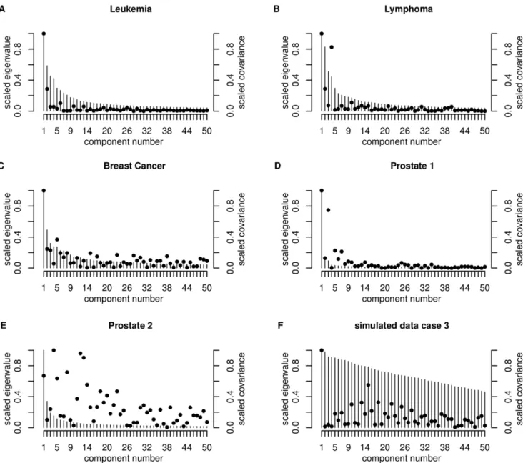
vector y. Here yi equals 1 if sample i belongs to group g~1, otherwiseyi equals -1,i~1,. . .,n. The eigenvector belonging to the kth largest eigenvalue is denoted byej. Helland and Almøy [14] infer, that data sets with relevant components, which have small eigenvalues, are difficult to predict. The condition index is plotted for the first five largest eigenvalues (scaled to the first eigenvalue) in Figure 3. Figure 4 shows the first 50 largest scaled eigenvalues and the corresponding scaled covariances betweenzj
andyfor all experimental data sets and a simulated data set (case 3) investigated.
Simulated data sets. Gene expression data are simulated as normally distributed data, considering the log scale of microarray intensities after normalization: xij
~N(mj,s2bzs2t),i~1. . .,n and
j~1,. . .,p. Here s2
b denotes the biological variance which we
chose equal to 0.04, and s2
t represents the technical variance which we chose in different proportions of the biological variance. Studying a two-class classification objective, we simulate 60 samples per class for the whole data set and p~1000 genes partitioned in an informative part and non-informative part for the classification. For the test set, 30 single samples per class are randomly chosen. The remaining 30 single samples per class constitute the training set. The non-informative part of the data matrix which shows no differences between the two classes, consists of normally distributed random variables with mean mg~8and biological variances2
b~0:04, as well as different cases of technical variance s2
t. The informative part contains ten differentially expressed genes (DEGs) with a mean class difference
D[7]. We take 5 cases into account. For case 1, 2 and 3, for each DEGs,Dis chosen according to the uniform distribution from the interval½0:1,0:5. Case 1 has a technical variance of zero, case 2 of
one-quarter of the biological variance (s2 t~
1 4s
2
b), and case 3 is simulated with a technical variance of the same size as the biological variance (s2
t~s2b). The ten DEGs of case 4 have a mean class difference ofD~0:2 ands2
t~ 1 4s
2
b. The simulated data of
case 5 also have the high noise level (s2 t~
1 4s
2
b), but a higher mean class difference withD~0:5.
We illustrate the data structure for the simulated data on the example of case 3. The condition indexes are 1.00, 1.01, 1.04, 1.05, 1.06. The increase is the weakest for all data sets considered (Figure 3), and therewith the genes are only weakly linear dependent, which is also shown by Figure 4F. This is similar for
Figure 1. Rough overview of the proposed extension of PPLS-DA.
doi:10.1371/journal.pone.0055267.g001
all simulated data cases. Furthermore, the proportion of DEGs is very low with1%for all cases.
Experimental data sets. Additionally, we considered five publicly available experimental microarray gene expression data sets which are summarized in Table 1 containing information about the group size, number of genes, proportion of differentially expressed genes and original publication. For the determination of the number of differentially expressed genes (NDEGs) we use a t-test (from the R-package stats) and an FDR correction [15] (R-package qvalue). We count all genes with a q-value below 0.05. In the following the five data sets are described:
The Leukemia data were downloaded from the Whitehead Institute website. We merge the training set and the test set to get a higher sample size and sample from these to get new proportions 0.7 and 0.3 for the training and test set. The R code for data preprocessing from http://svitsrv25.epfl.ch/R-doc/library/ multtest/doc/golub.R is used which is according to [16]. The data set consists of two groups, 25 patients with acute myeloid leukemia and 47 patients with acute lymphoblastic leukemia and 3571 genes.
The condition indexes show a weak increase for this data set (1.00, 1.31, 1.49, 1.537, 1.83). This and the plot of the eigenvalues (Figure 4A) lead to the assumption of a weak linear dependency between the genes. The more relevant components have the largest eigenvalues (Figure 4A). Therefore we can expect good prediction performance of this data set. This data set has the highest proportion of DEGs (40.46%, Table 1).
The Lymphoma data set was downloaded from the website http://www.broadinstitute.org/mpr/lymphoma/. The data are GC-RMA normalized. Two groups are considered, 58 patients
with diffuse large B-cell lymphomas and 19 patients with B-cell lymphoma, follicular lymphoma. Only genes with a non-zero variance are used in our analysis, which leads to 7129 genes.
The between-variable dependencies are comparable to the Leukemia data set (condition indexes: 1.00, 1.10, 1.40, 1.50, 1.84). The covariance structure (Figure 4B) is also comparable to those of the Leukemia data set and the total number of DEGs is a little bit higher than for the Leukemia data set, but the proportion on the total number of genes is clearly lower (24.3%, Table 1).
The Breast Cancer data set consists of normalized and filtered data, downloaded from http://homes.dsi. unimi.it/,valenti/ DATA/MICROARRAY-DATA/R-code/Do-Veer-data.R. The normalization was performed according to [17]. In this data set, only the two groups with the highest sample size are included: 34 patients with distant metastases within 5 years and 44 patients without, after at least 5 years. The total number of genes is 4997. We found again a weak increase in the condition indexes for the first five eigenvalues (1.00, 1.42, 1.77, 1.90 and 1.91), but slightly faster than for the Leukemia and Lymphoma data set (Figure 3). The eigenvalue plot (Figure 4C) illustrates also a weak linear dependence between the features. The proportion of DEGs is the lowest for all experimental data sets (1.08%, Table 1).
The Prostate 1 data set contains 52 tumor and 50 non-tumor cases and was downloaded from http://stat.ethz.ch/˜dettling/ bagboost.html. The preprocessing is described in [18] and the final data set contains 6033 genes.
This data set shows a rapid increase of the condition index from k1tok5(1.00, 2.96, 3.24, 5.046, 5.397), describing a strong linear dependency of the genes (Figure 3). This property is also indicated
Figure 2. Extension of PPLS-DA - for stepsizenª~0:1andNinner~50.The power parameter is denoted byc, the prediction error (number of wrongly classified samples of the inner test set) is abbreviated with PE.cvaried in 11 steps (c1~0,c2~0:1,. . .,c11~1). Cj, j = 1,. . .,5 is short for the jth component. The function min(f) takes the minimum of functionf. The cross-validation procedures consist of random samples of the outer training set to the proportions of 0.7 (training set) and 0.3 (test set). The cross-validation steps are conform to sampling with replacement. The optimalc-value and the optimal number of components are determined after 50 repeats.
by the plot of the eigenvectors (Figure 4D). This data set also has a high proportion of DEGs (32.26%, Table 1).
We downloaded the Prostate 2 data set, which was already normalized, from http://bioinformatics. mdanderson.org/Tail-Rank/. A description of the normalization can be found at http:// bioinformatics.mda nderson.org/TailRank/tolstoy-new.pdf. In this data set, only the two groups with 41 patients with normal prostate tissue and the 62 patients with primary tumors are in included.
The condition index shows a rapid increase (1.00, 1.71, 2.10, 2.56, 2.93) for the first five eigenvalues (Figure 3), but more moderate than for the Prostate 1 data set. Figure 4E shows that also relevant components have small eigenvalues, which indicates low prediction performance. The proportion of DEGs is very low (1.4%, Table 1) and similar to those of the Breast Cancer data set, but the total number of genes is the largest (42129) for all experimental data sets.
Results
Results for the simulated data are based on 100 repeated simulations, and for the experimental data 100 different outer training and outer test sets are sampled. We present mean PE values of the outer test sets and the corresponding 95%confidence intervals. At first, we describe and compare the results of PPLS-DA using copt with PPLS-DA using cmax, followed by the comparison between PLS-DA, PPLS-DA using c~0:5, t-LDA and SVM.
We calculate confidence intervals for PE as follows: letzbe the vector with 100 estimates of prediction errors. The upper bound of the confidence interval is then calculated as
u(z)~mean(z)z1:96(z)= ffiffiffiffiffiffiffiffi 100
p
. The lower bound is calculated likewise. If these confidence intervals overlap, we report no significant differences, if they are disjunct, the corresponding PEs are reported as significantly different.
Results for the Simulated Data
PE results. At first we study the dependency ofc optimiza-tion on the step size nc, and on the number of internal
cross-validation steps Ninner. We calculate the mean PE results for
Ninner~5,10,20,30,40,50,60,70,80 andnc~0:05or0:1. Because
the corresponding 95% confidence intervals overlap for all different parameter choices for fix Ninner (Figure S1), we show all further results forNinner~50andnc~0:1.
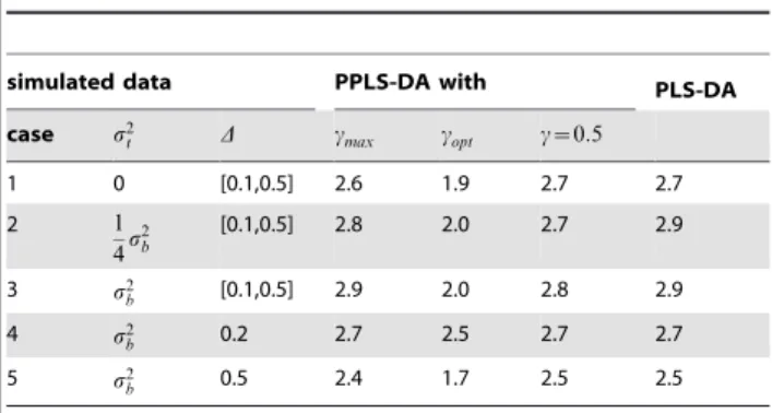
Figure 5 illustrates the mean PE results and corresponding 95% confidence intervals for the simulated data and Table 2 summa-rizes the average number of components used for PLS-DA, PPLS-DA usingcmax,coptandc~0:5.
For all considered cases, PPLS-DA using copt shows a significantly smaller PE than PPLS-DA usingcmax. Especially for DEGs withD[½0:1,0:5, the PE of PPLS-DA withc
optis only one-tenth of the PE for the PPLS-DA withcmax in the case without
noise, one-fifth for a minor noise level (s2 t~
1 4s
2
b) and still one-third for a high noise level withs2
t~s2b.
Figure 3. Condition index for the first five eigenvalues.The condition indexkj~
ffiffiffiffiffiffiffiffiffiffiffi l1=lj
p
,j~1,. . .,p(pnumber of features) is used as a measure for variable dependence, withljeigenvalue ofcov(X). It can be assumed thatl1§l2§ §lp. The increase of the first five condition
indexes (k1,k2,k3,k4,k5) reflects the collinearity of the features. A rapid increase means, the features are strong linear dependent, a weak increase implies a weak dependence.
doi:10.1371/journal.pone.0055267.g003
Figure 4. Plot of the first 50 largest eigenvaluesekof cov(X) (bars) and of the absolute covariance betweenzkandy(dots) for the experimental data sets and for case 3 for the simulated data.The eigenvaluesek,k~1,. . .,50are scaled corresponding to the largest eigenvalue, also the absolute values of the covariance between the principal componentzk~Xek,k~1,. . .,50and the response vectory, hereyi
equals 1 if sample i belongs to groupg~1, otherwiseyiequals21.
doi:10.1371/journal.pone.0055267.g004
Table 1.Overview of the experimental data sets.
name number of samples number of genes NDEGsa NDEGsin % original publication
Leukemia 47/25 3571 1445 40.46 [19]
Lymphoma 58/19 7129 1739 24.39 [20]
Breast cancer 44/34 4997 54 1.08 [17]
Prostate 1 50/52 6033 2393 35.26 [21]
Prostate 2 41/62 42129 595 1.40 [22]
aFor the determination of the number of differentially expressed genes (NDEGs) we use a t-test (from the R-package stats) and an FDR correction [15] (R-package qvalue).
Considering the frequency distributions ofcopt-values (Figure S2 shows the corresponding histograms for case 3), the value with the highest frequency for the optimalc-value (copt) determined in a cross-validation approach is 0.8. This is in contrast to the values for cmax, with 0.5 as highest frequency (Figures S2A and B, see Supplementary Materials).
Different power parameters have large effects on the loading weights, which can be seen in Figure 6, e.g. for the first component forcmaxandcoptwithNinner= 50 andnc= 0.1 for case 3. The first
10 genes, which are simulated as differentially expressed, receive the highest absolute loading weight values for all methods. For copt, these loading weights of the informative genes are increasing in absolute values, and especially the non-informative genes receive loading weight values near to zero in comparison to the loading weights induced bycmax.
Comparing our above findings of the PE with those of the PE of PLS-DA and of PPLS-DA withc~0:5, PLS-DA shows an equal PE to PPLS-DA usingcmaxorc~0:5, for all cases of the simulated data. Therewith also PPLS-DA usingc~0:5shows a significantly lower PE than PLS-DA. The number of components used for PLS-DA is equal to the corresponding number of components used for PPLS-DA usingcmaxorc~0:5. Hence overall, PPLS-DA usingcoptuses in average the lowest number of components.
Now, we consider the results of the two methods, SVM and t-LDA. For all simulated data cases, the method SVM shows the largest PE for all simulated data cases. The method t-LDA does not show a significant different PE to PPLS-DA usingcopt.
Results for the Experimental Data Sets
As for the simulated data, we chooseNinner~50andnc~0:1.
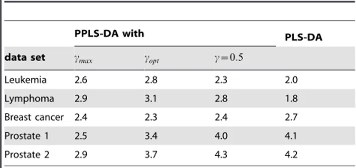
In Figure 7 the mean PE results and the corresponding 95% confidence intervals are shown for all five experimental data sets for all considered methods. For PPLS-DA using cmax, copt and c~0:5and PLS-DA, the average number of of components are shown in Table 3.
Leukemia data set: For this data set, we found no significant differences in the PE of PPLS-DA usingcoptcompared to PPLS-DA usingcmax(Figure 7A), and both methods use similar numbers of components. The modal value ofcoptis 0.5, in comparison to cmaxwith two accumulations one around 0.3 and the other around 0.8 (see Figure S3, see Supplementary Materials). Comparing the above PE results to PLS-DA, then PLS-DA shows an equal PE compared to all four extensions of PPLS-DA. The PE of PPLS-DA
using cmax is significantly larger than the PE of PPLS-DA with c~0:5 and PLS-DA. PLS-DA uses also in average the lowest number of components (2.0).
For PPLS-DA usingcoptwe find a significantly lower PE than for t-LDA, but for SVM the PE is similar to that of PPLS-DA usingcopt.
Lymphoma data set: The PE of PPLS-DA using copt is significantly lower than the PE of PPLS-DA using cmax (Figure 7B). PPLS-DA using copt leads in average to 3.1 components and PPLS-DA usingcmaxto 2.9 components.
Considering PLS-DA, we find a significantly lower PE than for PPLS-DA usingcmax, which is equal to the PEs of PPLS-DA using copt and c~0:5. PLS-DA used the smallest average number of components (1.8), for PPLS-DA usingcmax and c~0:5we find similar number of components in average 2.9 and 2.8.
The method t-LDA shows a significantly higher PE in comparison to PPLS-DA using copt, and SVM an equal PE to PPLS-DA usingcopt.
Breast cancer data set: For this data set, PPLS-DA using cmax and PPLS-DA usingcoptdoes not show significantly different PEs (Figure 7C). The number of components used are also similar for these two methods with 2.4 for PPLS-DA usingcopt and 2.3 for PPLS-DA usingcmax.
Also PLS-DA shows an equal PE and a slightly higher number of components (2.7), compared to PPLS-DA usingcoptandcmaxor c~0:5.
If compared to PPLS-DA using copt, t-LDA and SVM show similar PE.
Prostate 1 data set: PPLS-DA using copt shows equal PE to PPLS-DA using cmax (Figure 7D). PPLS-DA using copt leads in average to 3.4 components, while PPLS-DA usingcmax uses 2.5 components.
Investigating PLS-DA, the PE is equal to the PE of PPLS-DA usingcmaxorc~0:5. PPLS-DA usingc~0:5and PLS-DA use the largest average number of components, 4.1 and 4 (see Figure S4). Also t-LDA and SVM show equal PEs to the other methods. Prostate 2 data set: The PE of PPLS-DA usingcoptis equal to the PE of PPLS-DA withcmax (Figure 7E). Moreover, PPLS-DA usingcmaxused 2.9 components and PPLS-DA usingcoptuses 3.7 components.
PPLS-DA using c~0:5 and PLS-DA show equal PE and significantly higher PE than for PPLS-DA usingcmaxor usingcopt. PPLS-DA with c~0:5 and PLS-DA use more components in comparison to all versions of PPLS-DA.
Both methods t-LDA and SVM show a significantly larger PE than PPLS-DA using cmax or PPLS-DA using copt, but a significantly lower PE than PLS-DA and PPLS-DA usingc~0:5.
Discussion
The focus of our study is on introduction of an extension for the method PPLS-DA for better classification in high-dimensional datasets, as for example gene expression datasets in biomedicine. The optimization criterion for the power parametercmax in the ordinary PPLS-DA is towards canonical correlation, and does not need to be best for prediction. Our extension of PPLS-DA introduces optimization ofcwith respect to prediction using an inner cross-validation approach. We carry along comparisons to LDA and SVM, to bring our proposed method into line with these standard classification methods.
Figure 5. Mean PE of PPLS-DA usingªmax,ªoptandª~0:5,PLS-DA, t-LDA and SVM for the five cases of the simulated data.
doi:10.1371/journal.pone.0055267.g005
Table 2.The mean number of components used for simulated data forNinner~50andnc= 0.1.
simulated data PPLS-DA with PLS-DA
case s2
t D cmax copt c~0:5
1 0 [0.1,0.5] 2.6 1.9 2.7 2.7
2 1
4s
2 b
[0.1,0.5] 2.8 2.0 2.7 2.9
3 s2
b [0.1,0.5] 2.9 2.0 2.8 2.9
4 s2
b 0.2 2.7 2.5 2.7 2.7
5 s2
b 0.5 2.4 1.7 2.5 2.5
Comparison between PPLS-DA using cmax andcopt
The PEs of the outer test sets for PPLS-DA were improved or showed at least equal values by optimization of thec{value with respect to the prediction with LDA in comparison to PPLS-DA usingcmax, for all simulated data and the experimental data sets. Simulated data. Comparing the histograms of c{values found by PPLS-DA usingcoptand PPLS-DA withcmax, the reason for the lower PE can be traced back to the down-weighting of the non-informative features for the simulated data (see Figure S2 and Figure 6). The loading weights for these features are near or equal to zero. The influence of the features, which are not informative for the discrimination (and can be interpreted as noise), is reduced, because the impact on the calculation of the components is lower for PPLS-DA usingcoptthan for PPLS-DA withcmax. Values ofc near to one, leads to preference of features which show a high correlation to the dummy response (in the simulation study these are the differentially expressed genes). Changing the optimization criterion from correlation towards prediction, leads also to a lower average number of components for the simulated data.
Experimental data. For the experimental data, thec-values determined by the canonical correlation (cmax) are larger than the c{values detected by our proposed extension of PPLS-DA. Even if our analyses of simulated data suggested lower PE values for larger choices ofc, for the Leukemia data set and the Lymphoma data set also PPLS-DA usingcoptshows a significantly lower PE than PPLS-DA usingcmax. Note, that the true informative genes for the experimental data are not known, and the proportion of differentially expressed genes most likely is much larger than for the simulated data, therefore the comparison of the results for simulated and experimental data is not straightforward. Moreover experimental data are usually noisier than simulated data. The part of reality we have not been able to model in the simulated data might be a sort of noise and data structure that we cannot improve on, regardless our choice of c. If we could remove this
part of the noise from the real data, the relative improvements might be just as good as with the simulated data.
Summarizing the findings for the simulated data, PPLS-DA usingcoptshows significantly lower PEs than PPLS-DA withcmax. For the experimental data, the results are also significantly lower or equal for the extensions considering the PE.
Additionally we had considered three further versions to determine the power parameter towards prediction. These versions for example differ in the number of considered components for the optimization of the power parameter and also one version which optimizes an individual power parameter for each component was studied. The results are similar to those of the extension presented here (data not shown).
Comparison between PPLS-DA usingcmaxand PLS-DA
The development of PPLS-DA followed the development of powered partial least squares as a natural extension of the power methodology to handle discrete responses. Several factors moti-vated this advancement to PLS-DA. First the application of powers enables focusing on fewer explanatory variables in the loading weights, smoothing over some of the noise in the remaining variables. Second, focus can be shifted between the correlation and standard deviation parts of the loading weights, which is even more important for discrete responses. Finally, the maximization criterion is moved from the between-group varia-tion (B) to the product of the between group variavaria-tion matrix and the inverse of the within-group variation matrix (W{1B~T{1B
). This has the effect of moving from covariance maximization to a correlation maximization. Instead of just searching for the space having highest variation between the groups, we also minimize the variation inside the groups, increasing the likeliness of good group separation.
In our study, PPLS-DA with c~0:5 (applying no power parameter) and PLS-DA always show equal PEs for the simulated and the experimental data sets. Hence, for this case the different
Figure 6. Average loading weights of the first component for the simulated data (case 3).The simulated data of case 1 are constructed such that the technical variance is of the same size as the biological variance. 10 differentially expressed genes with a mean class difference D[½0:1,0:5are simulated. Loading weights for the first component as calculated by PPLS-DA are shown with the power parametercmax(A) andcopt (B) using 50 inner cross-validation steps and a stepsize ofnc~0:1. The basis are the results of 100 choices of the outer training and outer test set. doi:10.1371/journal.pone.0055267.g006
optimization tasks show no great differences with respect to the PEs of the outer test sets. Including the power parameter, the PE of PPLS-DA using cmax is equal to the PE of PLS-DA for all simulated data. Also, the number of components used is in average lower or equal for PPLS-DA usingcmax than for PLS-DA.
For two of the five experimental data sets (Leukemia and Lymphoma), the PE of PPLS-DA usingcmaxis significantly higher than the PE of PLS-DA. For these data sets, the proportions of differentially expressed genes are large (24.4% and 40.5%) and the genes are only weakly linear dependent (considering the condition indexes). The PE of PPLS-DA using cmax is significantly lower than for PLS-DA for the Prostate 2 data set, and the number of components used is also in average lower. This data set contains only a low proportion of 1.4% differentially expressed genes, and the total number of genes is very high (42129). Moreover, for this data set, the genes show a stronger linear dependency (rapid increase of the condidion index) than for the Leukemia or the Lymphoma data set.
Summarizing, a weak increase of kj,j~1. . .,5 indicates no improvement for the PE when using PPLS-DA withcmax instead of PLS-DA. Concerning percentage of DEGs, the PE of PPLS-DA using cmax is equal to the PE of PLS-DA only for a small percentage of DEGs (Breast Cancer data and case 3 of the simulated data). For a weak increase of kj,j~1. . .,5 and high percentage of DEGs, the PE for PPLS-DA using cmax is even larger than for PLS-DA (Leukemia and Lymphoma data sets).
A rapid increase of kj,j~1. . .,5 and a large proportion of DEGs, usingcmax instead of PLS-DA does not improve the PE (Prostate 1). On the contrary, for a rapid increase ofkj and the case of small percentage of DEGs, we can improve the PE, employing PPLS-DA usingcmax instead of PLS-DA (Prostate 2).
Comparison between PLS-DA and PPLS-DA usingcopt For the simulated data, PLS-DA shows equal PE if compared to PPLS-DA usingcmaxorc~0:5. The PE of PPLS-DA usingcoptis significantly lower than the PE of PLS-DA. For the experimental data, for four of the five data sets (Leukemia, Lymphoma, Breast Cancer and Prostate 1), the PEs of PLS-DA and PPLS-DA using coptshow no significant differences. For the Prostate 2 data set, the PE of PPLS-DA usingcoptis clearly lower than for PLS-DA.
We conclude first, equal PEs between PLS-DA and PPLS-DA using copt are caused by a weak between-feature dependency, independent of the proportion of DEGs. Second, a data set with
strong collinearity between the features and a low number of DEGs, in contrary shows a clearly lower PE for PPLS-DA using coptthan for PLS-DA.
Comparison between PPLS-DA usingc~0:5and PLS-DA
The PEs for PLS-DA and PPLS-DA using c~0:5 are non-distinguishable for all simulated and all experimental data sets investigated. Maximization of the covariance or maximization of the correlation without the power parameter, results in equal PEs of the outer test set.
Comparison between PPLS-DA usingcoptand t-LDA and
SVM
The more classic and widely available classification methods t-LDA and SVM were also run and compared to PPLS-DA using copton all simulated and experimental data sets. For the simulated data, t-LDA performs indistinguishable well as PPLS-DA using copt. For the experimental datasets, SVM draws level with our proposed approach except for the case of Prostate 2. In this comparison, PPLS-DA using copt shows a comparatively stable well performance. There may, however, exist further statistical learning methods which outperform the methods presented in this study. t-LDA and SVM should serve to demonstrate comparability of PLS-related methods to other commonly chosen approaches for the classification problems. The focus of our study, however, was on further developing PPLS-DA, a so-called multivariate method, which has already been proven its large potential for classification problems involving magnitude more features than samples as it is the case in OMICs data sets.
Conclusions and Outlook
It is conceivable to use results of an initial PPLS-DA cross-validation series, optimizingcmax, to try to judge if running the extended version would be rewarding. Data sets with a high proportion of differentially expressed genes and weak linear dependency (like the Leukemia data set and the Lymphoma data set) most probably show good prediction results for PLS-DA. Here, we found no gain using PPLS-DA with powers (cmaxorcopt). On the contrary, for a rapid increase of the condition index, a low proportion of differentially expressed genes and a large total number of genes, using PPLS-DA withcmaxclearly improves the prediction error compared to PLS-DA. In cases where PPLS-DA usingcmaxgives no advantages over PLS-DA, using the extensions of PPLS-DA (optimizing the power parameter) for prediction can be advantageous. Starting to analyse the eigenvalue structure and the number of differentially expressed genes, can possibly be useful to decide which method to use. One aspect of future work is to validate our conclusions by additional experimental data sets as well as further simulations implementing a more complex covariance structure.
Supporting Information
Figure S1 Mean PE of PPLS-DA for simulated data usingcopt plotted against Ninner. The simulated data of case 3 are constructed such that the technical variance is of the same size as the biological variance. 10 differentially expressed genes with a mean class difference D[½0:1,0:5 are simulated. For different numbers of the cross-validation steps, the mean prediction error
Figure 7. Mean PE of PPLS-DA usingcmax,coptandc~0:5, PLS-DA, t-LDA and SVM for the five cases of the experimental data sets.
doi:10.1371/journal.pone.0055267.g007
Table 3.The mean number of components used for the experimental data sets.
PPLS-DA with PLS-DA
data set cmax copt c~0:5
Leukemia 2.6 2.8 2.3 2.0
Lymphoma 2.9 3.1 2.8 1.8
Breast cancer 2.4 2.3 2.4 2.7
Prostate 1 2.5 3.4 4.0 4.1
Prostate 2 2.9 3.7 4.3 4.2
doi:10.1371/journal.pone.0055267.t003
(PE) and the corresponding 95%confidence intervals are shown for PPLS-DA using copt for the determination of the power parameter. Two stepsizesncare considered for the fragmentation
of the interval [0,1],nc~0:05(A) andnc~0:1(B). The basis are
the results of 100 choices of the outer training and outer test set. (TIFF)
Figure S2 Histograms of cmax and coptfor the simulated data (case 3). The simulated data of case 1 are constructed such that the technical variance is of the same size as the biological variance. 10 differentially expressed genes with a mean class difference
D[½0:1,0:5are simulated. Values ofc
max detected by PPLS-DA for the first component (A) and for all components (B). In panel (C) the c-values are shown, detected for copt with Ninner~50 and stepsizenc~0:1. The basis are the results of 100 choices of the
outer training set. (TIFF)
Figure S3 Histograms ofcmax and coptfor the Leukemia data set. Values ofcmaxdetected by PPLS-DA for the first component (A) and for all components (B). In panel (C) thec-values are shown,
detected forcoptwithNinner~50and step sizenc~0:1. The basis
are the results of 100 choices of the outer training set. (TIFF)
Figure S4 Histograms ofcmax andcopt for the Prostate 1 data set. Values ofcmax detected by PPLS-DA for the first component (A) and for all components (B). In panel (C) thec-values are shown, detected forcoptwithNinner~50and step sizenc~0:1. The basis
are the results of 100 choices of the outer training set. (TIFF)
Acknowledgments
The authors thank K. Schlettwein for comments and discussion of implementation possibilities, and H. Rudolf for critical comments and normalization of the Lymphoma data set.
Author Contributions
Conceived and designed the experiments: AT KHL DR GN. Performed the experiments: AT. Implemented algorithms and extensions and analysed simulated and experimental data: AT. Analyzed the data: AT GN. Wrote the paper: AT KHL DR GN.
References
1. Wold S, Albano C, Dunn II W, Esbensen K, Hellberg S, et al. (1983) Pattern recognition: Finding and using regularites in multivariate data, applied Sciences publ. London. 147–188.
2. Martens SWH, Wold H (1983) The multivariate calibration problem in chemistry solved by the pls method. Proc Conf Matrix Pencils (ARuhe, BKaagstroem, eds) March 1982 Lecture notes in Mathematics : 286–293. 3. Barker M, Rayens W (2003) Partial least squares for discrimination. Journal of
Chemometrics 17(3): 166–173.
4. Nocairi H, Qannari EM, Vigneau E, Bertrand D (2005) Discrimination on latent components with respect to patterns. application to multicollinear data. Computational Statistics & Data Analysis 48 (1): 139–147.
5. Liland KH, Indahl U (2009) Powered partial least squares discriminant analysis. Journal of Chemometrics 23: 7–18.
6. Indahl UG (2005) A twist to partial least squares regression. Journal of Chemometrics 19: 32–44.
7. Telaar A, Repsilber D, Nu¨rnberg G (2011) Biomarker Discovery: Classification using pooled samples - a simulation study. Computational Statistics. 8. Indahl UG, Martens H, Næs T (2007) From dummy regression to prior
probabilities in pls-da. Journal of Chemometrics 21: 529–536.
9. Indahl UG, Liland KH, Næs T (2009) Canonical partial least squares - a unified pls approach to classification and regression problems. Journal of Chemometrics 23: 495–504.
10. Dimitriadou E, Hornik K, Leisch F, Meyer D, Weingessel A (2009) e1071: Misc functions of the department of statistics (e1071). TU Wien.
11. Dettling M (2004) Bagboosting for tumor classification with gene expression data. Bioinformatics 20: 3583–3593.
12. Sæbø S, Almøy T, Aarøe J, Aastveit AH (2008) ST-PLS: a multi-directional nearest shrunken centroid type classifier via PLS. Journal of Chemometrics 20: 54–62.
13. Belsley DA, Kuh E, Welsch RE (1980) Regression Diagnostics: Identifying Inuential Data and Sources of Collinearity. John Wiley & Sons.
14. Helland IS, Almøy T (1994) Comparison of prediction methods when only a few components are relevant. Journal of the American Statistical Association 89: 583–591.
15. Storey J, Tibshirani R (2003) Statistical signilficance for genomewide studies. Proc Natal Acad Sci 100: 9440–5.
16. Dudoit S, Fridlyand J, Speed TP (2002) Comparison of discrimination methods for the classification of tumors using gene expression data. Journal of the American Statistical Association 97: 77–87.
17. van’t Veer LJ, Dai H, van de Vijver MJ, He YD, Hart AA, et al. (2002) Gene expression profiling predicts clinical outcome of breast cancer. Nature 415: 530– 536.
18. Dettling M, Buehlmann P (2003) Boosting for tumor classification with gene expression data. Bioinformatics : 1061–1069.
19. Golub TR, Slonim DK, Tamayo P, Huard C, Gaasenbeek M, et al. (1999) Molecular classification of cancer: class discovery and class prediction by gene expression monitoring. Science 286: 531–537.
20. Shipp MA, Ross KN, Tamayo P, Weng AP, Kutok JL, et al. (2002) Diffuse large b-cell lymphoma outcome prediction by gene-expression profiling and supervised machine learning. Nat Med 8: 68–74.
21. Singh D, Febbo PG, Ross K, Jackson DG, Manola J, et al. (2002) Gene expression correlates of clinical prostate cancer behavior. Cancer Cell 1: 203– 209.