Abstract Control charts are widely implemented in firms to establish and maintain statistical control of a process which leads to the improved quality and productivity. Design of control charts requires that the engineer selects a sample size, a sampling frequency and the control limits for the chart. In this paper, a possible combination of design parameters is considered as a decision making unit which is identified by three attributes: hourly expected cost, detection power of the chart and in-control average run length. Optimal design of control charts can be formulated as multiple objective decision making (MODM). The cost function is extended from single to multiple assignable causes because there exist multiple assignable causes in real practice. An algorithm using DEA is applied to solve the MODM model. A numerical example is used to illustrate the algorithm procedure. Finally, sensitivity analysis has been carried out to investigate the robustness of the model
Index Terms Control chart design, Data envelopment analysis, X control chart, Multiple-objective decision making
(MODM)
I.INTRODUCTION
If a product is to meet or exceed customer expectations, it should be produced by a process that is stable or repeatable. Statistical process control is a powerful collection of problem solving tools useful in achieving process stability and improving capabilities through the reduction of variability. The main tool of statistical process control is the statistical control chart. The engineering and technical implementation of control charts entails selecting sample sizes, sampling frequencies and the control limits for the chart. Selection of these three parameters is called the design of control chart. Traditionally, control charts have been designed with respect to statistical criteria only, but the design of a control chart has economic aspects too.
The first model in this case was proposed by Duncan [1]. Since that time, the economic approach has received considerable attention and various models have been suggested in this area. But as declared by Woodall [2], control charts based on optimal economic design, have poor
Manuscript submitted July 23,2008
Corresponding Author: Shervin Asadzadeh, MS student, Department of Industrial Engineering, K.N.Toosi University of Technology. No.17, Pardis St., Molla-Sadra St., Vanak Sq., Tehran, Iran. P.O.BOX. 19395-1999; phone: +982188674999; fax: +982188674858
e_mail: [email protected].
Farid Khoshalhan, Assistant Professor, Department of Industrial Engineering, K.N.Toosi University of Technology No.17, Pardis St., Molla-Sadra St., Vanak Sq., Tehran, Iran. P.O.BOX. 19395-1999; phone: +982188674999; fax: +982188674858
e_mail: [email protected]
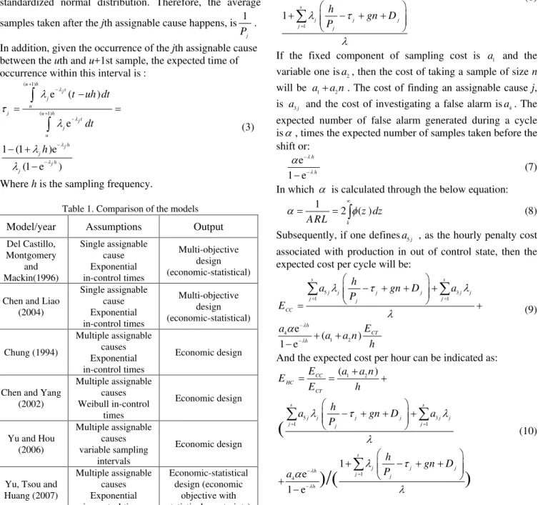
statistical properties. To solve this problem, Saniga [3] noted that some of the criticism of economic design can be overcome by introducing statistical constraints in the problem and solving the model using nonlinear optimization techniques. Del Castillo, Montgomery and Mackin [4] proposed an interactive multi objective algorithm based on this procedure. In addition, Chen and Liao [5] formulated optimal design of control charts as a multiple criteria decision making with respect to the constraints proposed by Saniga.
In the mentioned articles, a single assignable cause cost function was used. However in 1971, Duncan [6] developed his previous model and presented a new model in the presence of multiple assignable causes. Since then, many tried to optimize this cost function. Chung [7] carried out subsequent work on Duncan s model [6]. Chen and Yang [8] considered weibull in-control times with multiple assignable causes. Yu and Hou [9] optimized the control chart parameters with multiple assignable causes and variable sampling intervals. Also, Yu, Tsou and Huang [10] used Duncan's model and the proposed constraints by saniga
[3] to investigate economic-statistical design of X control
chart. Table 1 shows the comparison of different models, mentioned above.
However, multiple objective design of X control charts
with multiple assignable causes has not been addressed in the literature. Therefore, the purpose of this paper is to find
the optimum design parameters of X control charts using
DEA, in presence of multiple assignable causes which satisfy all economic and statistical objectives. A numerical example is given to illustrate the model's working. Sensitivity analysis has been done to ensure the aptness of the model.
II. ECONOMIC COST FUNCTION WITH MULTIPLE ASSIGNABLE CAUSES
Duncan [6] generalized his single assignable cause model to multiple one. In this model, there is an in-control state , an
assignable cause of magnitude j (j 1 2, ..., s) which
occurs at random, results in a shift in the mean to either
j or j and so changes the state until the
cause is detected. Meanwhile, during the search for the assignable cause, the process is allowed to continue in operation. The cycle consists of four periods:
1) In-control period
It is assumed that assignable causes occur according to
Poisson process with joccurrences per hour. So, assuming
A DEA Based MODM Model for Designing
X
Control Chart
Shervin Asadzadeh , Farid Khoshalhan
IAENG International Journal of Applied Mathematics, 38:3, IJAM_38_3_06
that process begins in the in-control state, the time interval that the process remains in control is an exponential random
variable with mean 1 hour:
1 1 1 s j i (1)
2) Out of control period
When the process goes to out of control state, the probability that it will be detected on any subsequent sample
is related to the assignable cause occurred. If the jth
assignable cause happens, then the detection power will be:
( ) + ( )
k j n j
k j n
P z dz z dz (2)
where ( )z , is the probability density function of
standardized normal distribution. Therefore, the average
samples taken after the jth assignable cause happens, is 1
j
P .
In addition, given the occurrence of the jth assignable cause
between the uth and u+1st sample, the expected time of
occurrence within this interval is :
( 1)
( 1)
e ( )
e
1 (1 )e
(1 e )
u h t j j u
j u h
t j j u h j j h j j
t uh dt
dt
h
(3)
Where h is the sampling frequency.
Table 1. Comparison of the models
Output Assumptions Model/year Multi-objective design (economic-statistical) Single assignable cause Exponential in-control times Del Castillo, Montgomery and Mackin(1996) Multi-objective design (economic-statistical) Single assignable cause Exponential in-control times Chen and Liao
(2004) Economic design Multiple assignable causes Exponential in-control times Chung (1994) Economic design Multiple assignable causes Weibull in-control times Chen and Yang
(2002) Economic design Multiple assignable causes variable sampling intervals Yu and Hou
(2006) Economic-statistical design (economic objective with statistical constraints) Multiple assignable causes Exponential in-control times Yu, Tsou and
Huang (2007)
Therefore, the time required to observe an out of control
alarm when the jth assignable cause occurs, will be:
j j
h
P (4)
3) The time to take sample and interpret the results is a
constant g proportional to the sample size n, so that gn is the
length of this part of the cycle.
4) The time required to find the assignable cause. If this
time is Dj for the jth assignable cause, then the expected
time in a cycle for detecting assignable cause is:
1 s j j j D (5)
Therefore, the expected length of a cycle is:
1 1 1 1 1 s s
j j j j
j j
j CT
s
j j j
j j h D P E gn h gn D P (6)
If the fixed component of sampling cost is a1 and the
variable one isa2, then the cost of taking a sample of size n
will be a1 a n2 . The cost of finding an assignable cause j,
is a3j and the cost of investigating a false alarm isa4. The
expected number of false alarm generated during a cycle
is , times the expected number of samples taken before the
shift or: e 1 e
h
h (7)
In which is calculated through the below equation:
1
2 ( )
k
z dz
ARL (8)
Subsequently, if one definesa5j , as the hourly penalty cost
associated with production in out of control state, then the expected cost per cycle will be:
5 3 1 1 4 1 2 e ( ) 1 e s s
j j j j j j
j j j
CC h
CT h
h
a gn D a
P E
E a
a a n h
(9)
And the expected cost per hour can be indicated as:
1 2 5 3 1 1 1 4 ( ) 1 e 1 e
(
) (
/
)
CC HC CT s sj j j j j j
j j j
s
j j j
h
j j
h
E a a n
E
E h
h
a gn D a
P h gn D P a (10)
IAENG International Journal of Applied Mathematics, 38:3, IJAM_38_3_06
Therefore, economic design of X control chart involves
determination of optimal parameters n, h and k which
minimizeEHC.
III. MULTIPLE OBJECTIVE OPTIMAL DESIGN OF X
CONTROL CHART
To establish the multiple objective decision making model, we should first determine a set of conflicting objectives that define the problem for the quality control manager. Due to the nature of the DEA method used in algorithm, various
combinations of design parameters n, h and k should also be
set in advance. Taking into account the Saniga s constraints [3], the multi-objective model is:
Max ARL D( )
Max P D( )
MinEHC( )D
s.t. (11)
( 1 2 )
j lj
P P j , ,..., s
u
( 1 2 )
j uj
ATS ATS j , ,..., s
ARL is the in-control average run length (reciprocal of false
alarm rate ( )), P is the detection power of the control
chart and EHCis the expected cost per hour. Pj and ATSj
are respectively the detection power and the average time to
signal when the jth assignable cause occurs and D is a
possible combination of design parameters that has been shown in bracket for the entire three objectives for emphasizing on the fact that it does have an impact on the values of objectives.
The aims of MODM models are to find solutions that can satisfy and set a balance among all objectives. To solve MODM problems, the DEA method is one of the most powerful and popular method to optimize the feasible combinations of design parameters specifically when measuring the efficiencies of similar units is under consideration.
IV. DATA ENVELOPMENT ANALYSIS (DEA)
DEA is the optimization method of linear programming to generalize the Farrell [11] single input, single output technical efficiency measure to the input, multiple-output case by constructing a relative efficiency score of a group of competing decision making units (DMU). Applications and implementations of DEA in modeling performance measurement have gained a lot of attention in recent years [12]. In this paper we have used the CCR model (Charnes, Cooper and Rhodes [13]). The objective in CRR model is to maximize the relative efficiency value of each of DMUs from among a reference set of design D, by selecting the optimal weights associated with the inputs and outputs. The algebraic model is as follows:
1
1
( )
Max ( )=
( )
z r ri r
i m
j ji j
U Y D
E D
V X D
s.t. (12)
1
1
( )
1 for other designs D
( )
z r ri r m
j ji j
U Y D
V X D
Where
Ur : the weights given to output r
Yri : amount of output r from unit i
Vj : weight given to input j
Xji : amount of input j from unit i
To solve the model, it is necessary to convert it into linear form so that methods of linear programming can be applied. This nonlinear programming is equivalent to two linear programming: 1) setting its denominator to one and maximizing its numerator (output maximization) 2) setting its numerator to one and minimizing denominator (input minimization). Because CCR model considers constant retunes to scale, there exists no difference which one to choose and CCR yields the same efficiency score. Therefore, the linear programming will be:
1
Max ( )= ( )
z
i r ri
r
E D U Y D
s.t. (13)
1
( ) 1
m j ji j
V X D
1 1
( ) ( ) 1 for other designs D
z m
r ri j ji
r j
U Y D V X D
0
r j
U ,V
If *
1
i
E , that means no other design is more efficient than
design i under its own weights. If *
1
i
E , then there is at
least one other design that is more efficient under optimal set of weights determined. Calculation should be done for each DMU to find the relative efficiency of each one.
V. SOLUTION ALGORITHM
Unlike many multiple-objective models that the DM has an implicit unknown value function, here the values of
( )
HC
E D , ( )P D and ARL D( )must be calculated for each
potential combination D according to formula 1 to 10 in
advance. Due to the complicated multi-assignable cause cost function, all calculations have been facilitated by Excel software. In addition, to evaluate and compare the efficiencies of DMUs, Microsoft Excel with XlDEA has been implemented. Chen and Liao [5] proposed a solution procedure for their multi-criteria decision making model. In this paper, we have employed their 4-step algorithm to solve our multi-objective model. They applied this procedure for their model with one assignable cause cost function. The procedure is approximately the same except steps 1 and 2 which have been modified to suit our proposed MODM model.
The four-step procedure will be as follows:
1) Determining all possible solutions by putting bounds on
each parameter. In this paper the scope of sample size (n) is
set from 1 to 35, increased by 1. Scope of sampling
frequency (h) is confined from 0.1 to 4 increased by 0.1h
and finally the scope of control limit width (k) is considered
from 0.1 to 3 in terms of standard deviation increased by
IAENG International Journal of Applied Mathematics, 38:3, IJAM_38_3_06
0.1. Contemplating all possible combinations the number of potential solutions will be 35*40*30=42000
2) In this step we have added another constraint too, in
order to take into account the value of parameter h, because
in the two previous constraints Chen and Liao [5] used,
there was no sign of parameter h. subsequently, we
eliminate infeasible solutions by the following constraints:
u Pj Plj ATSj ATSuj
3) Partial optimization. Remain the elements with Pareto
optimality for each subset Qn . A solution "s" with Pareto
optimization in a set Qn means that there is no other
solution in the same set such that "s" is dominated in terms
of statistical properties and cost.
4) Global optimization. Merge all the remainders into a set W and select the elements with highest relative efficiency among W. The selected elements will afford to DM to make final decision.
VI.NUMERICAL EXAMPLE
In this section, Duncan s [6] data were employed to illustrate the use of the proposed model and algorithm. The numbers of assignable causes are assumed to be 12.
When an assignable cause j with the average occurrence of
j occurs, it produces a shift of size j in the mean. The
cost of taking a sample that is independent of sampling is $1 and the variable cost per item of sampling, testing and plotting is $0.1. An average time of 0.05h is needed to test and analyze a sample item and the cost of looking for trouble when none exists, is estimated $25. Values of other parameters have been tabulated in table 2.
Table 2. Input values of parameters
5j
a 3j
a
j
D
j j
7.22 19.68
4.17 0.001098 0.75
27.6 14.57
3.08 0.000855 1.25
76.14 11.81
2.50 0.000666 1.75
165.69 9.84
2.08 0.000519 2.25
302.36 9.06
1.92 0.000404 2.75
433.64 8.66
1.84 0.000314 3.25
570.32 8.37
1.77 0.000245 3.75
659.86 8.17
1.72 0.000191 4.25
708.4 8.05
1.70 0.000148 4.75
728.97 7.93
1.68 0.000115 5.25
735.78 7.83
1.66 0.000090 5.75
737.56 7.73
1.64 0.000070 6.25
Moreover, our statistical constraints in false alarm rate ,
detection power Pjand average time to signal ATSj are:
0 1. Pj 0 9. ATSj 4
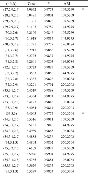
The optimization procedure can be carried out as described in previous section. Table3 illustrates the results.
As indicated by , two design parameters combinations have received score 1 and therefore offered to the DM for final selection. Then the DM may choose the first
combination if low cost is of paramount importance for him/her. Similarly if he/she is much more interested in the outgoing quality, then the second combination with large average run length and detection power may be the final choice.
Table 3. Non-dominated solutions with largest efficiencies
(n,h,k) Cost P ARL
(27,2.9,2.6) 5.9662 0.9773 107.5269 * (28,2.9,2.6) 6.0481 0.9801 107.5269 (29,2.9,2.6) 6.1301 0.9825 107.5269 (29,2.9,2.7) 6.1103 0.9789 144.9275 (30,3,2.6) 6.2109 0.9846 107.5269 (30,3,2.7) 6.1918 0.9814 144.9275 (30,2.9,2.8) 6.1771 0.9777 196.0784 (31,3,2.6) 6.2917 0.9866 107.5269 (31,3,2.7) 6.2725 0.9837 144.9275 (31,3,2.8) 6.2601 0.9803 196.0784 (32,3.1,2.6) 6.3723 0.9883 107.5269 (32,3,2.7) 6.3533 0.9856 144.9275 (32,3,2.8) 6.3387 0.9826 196.0784 (32,3,2.9) 6.3291 0.9791 270.2703 (33,3.1,2.6) 6.4519 0.9898 107.5269 (33,3.1,2.7) 6.4334 0.9874 144.9275 (33,3.1,2.8) 6.4193 0.9846 196.0784 (33,3,2.9) 6.4084 0.9814 270.2703
(33,3,3) 6.4003 0.9777 370.3704 * (34,3.1,2.6) 6.5316 0.9911 107.5269 (34,3.1,2.7) 6.5131 0.989 144.9275 (34,3.1,2.8) 6.4989 0.9865 196.0784 (34,3.1,2.9) 6.4883 0.9836 270.2703 (34,3.1,3) 6.4804 0.9802 370.3704 (35,3.2,2.6) 6.6109 0.9922 107.5269 (35,3.1,2.7) 6.5926 0.9904 144.9275 (35,3.1,2.8) 6.5785 0.9881 196.0784 (35,3.1,2.9) 6.5679 0.9855 270.2703 (35,3.1,3) 6.5599 0.9824 370.3704
VII.SENSITIVITY ANALYSIS
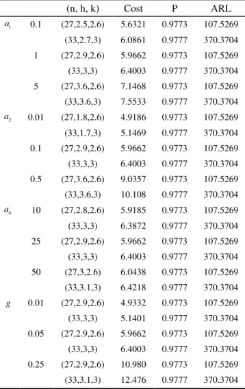
Sensitivity analysis has been done to study the effect of model parameters on the solution and to discuss the robustness of the proposed model. Fixed parameters effects such as constant sampling cost, variable sampling cost, cost of investigating the false alarm rate and finally the time for sampling and analyzing, have been studied. Table 4 illustrates the effect of these parameters on optimum solutions.
Some critical observations achieved from sensitivity analysis are as follows.
1) Decreasing fixed and variable sampling cost result in
reduction in sampling interval (h) and hourly expected cost.
IAENG International Journal of Applied Mathematics, 38:3, IJAM_38_3_06
2) The cost of searching for trouble when none exists (a4),
is relatively robust to the optimal solutions and expected cost.
3) The time to test and analyze a sample item (g) has
negligible effect on optimum solution but increasing it, may lead to considerable increase in hourly expected cost.
Table 4. Effect of parameters on optimum solutions
(n, h, k) Cost P ARL
1
a 0.1 (27,2.5,2.6) 5.6321 0.9773 107.5269
(33,2.7,3) 6.0861 0.9777 370.3704 1 (27,2.9,2.6) 5.9662 0.9773 107.5269
(33,3,3) 6.4003 0.9777 370.3704 5 (27,3.6,2.6) 7.1468 0.9773 107.5269
(33,3.6,3) 7.5533 0.9777 370.3704
2
a 0.01 (27,1.8,2.6) 4.9186 0.9773 107.5269
(33,1.7,3) 5.1469 0.9777 370.3704 0.1 (27,2.9,2.6) 5.9662 0.9773 107.5269
(33,3,3) 6.4003 0.9777 370.3704 0.5 (27,3.6,2.6) 9.0357 0.9773 107.5269
(33,3.6,3) 10.108 0.9777 370.3704
4
a 10 (27,2.8,2.6) 5.9185 0.9773 107.5269 (33,3,3) 6.3872 0.9777 370.3704 25 (27,2.9,2.6) 5.9662 0.9773 107.5269
(33,3,3) 6.4003 0.9777 370.3704 50 (27,3,2.6) 6.0438 0.9773 107.5269
(33,3.1,3) 6.4218 0.9777 370.3704
g 0.01 (27,2.9,2.6) 4.9332 0.9773 107.5269 (33,3,3) 5.1401 0.9777 370.3704 0.05 (27,2.9,2.6) 5.9662 0.9773 107.5269
(33,3,3) 6.4003 0.9777 370.3704 0.25 (27,2.9,2.6) 10.980 0.9773 107.5269
(33,3.1,3) 12.476 0.9777 370.3704
VIII.CONCLUSION
A multi-objective model for designing X control chart in
presence of multiple assignable causes is proposed. For this
model, various combinations of n, h and k are contemplated
as decision making units (DMUs). DEA method is employed to assess the efficiency of DMUs and to select the optimum designs with large average run length, high detection power and low expected cost. Numerical example is given based on the Duncan s [6] data to illustrate the solution procedures. Sensitivity analysis is carried out which indicates that optimal design of sampling frequency parameter is affected by fixed and variable sampling cost. Cost of searching for false alarm has approximately insignificant effect on design parameters and hourly expected cost and finally, increasing the time of test and analysis of a sample may lead to high expected cost. Other interesting research areas for future research involve
multi-objective design of X control chart under weibull shock
and multi-objective design of adaptive X control chart.
REFERENCES
[1] Duncan A.J (1956) The economic design of x charts used to maintain current control of a process .Journal of the American Statistical Association 51(274): 228-242.
[2] Woodall W.H (1986) Weakness of the economic design of control charts . Technometrics 28(4): 408 410.
[3] Saniga E. M (1989) Economic statistical control chart designs with an application to X and R charts . Technometrics 31(3): 313-320. [4] Del Castillo E, Mackin P, Montgomery D. C (1996) Multiple-criteria
optimal design of X control charts . IIE Transactions 28(6): 467-474
[5] Chen Y.K, Liao H.C (2004) Multi-criteria design of an X control chart . Computers and Industrial Engineering 46(4): 877-891 [6] Duncan A.J (1971) The economic design of x charts when there is a
multiplicity of assignable causes Journal of the American Statistical Association 66(333): 107-121
[7] Chung k.j (1994) An algorithm for computing the economically optimal X control charts for a process with multiple assignable causes . European Journal of Operation Research 72(2): 350-363 [8] ChenY.S, Yang Y.M (2002) Economic design of X control charts
with weibull in-control times when there are multiple assignable causes . International Journal of Production Economics 77(1): 17-23 [9] Yu F.J, Hou J.L (2006) Optimization of design parameters for
control charts with multiple assignable cause . Journal of Applied Statistics 33(3): 279 290
[10] Yu F.J, Tsou C.S , Huang K.I (2007) An Economic-Statistical Design of X Control Charts with Multiple Assignable Causes . The 22 nd European Conference on Operational Research.
[11] Farrell M.J (1957) The measurement of productive efficiency . J.R. Statis. Soc. Series A 120(3): 253-290
[12] Cook W.D , Zhu J (2005) Modeling Performance Measurement, Springer
[13] Chanes A, Cooper W.W, Rhodes E (1978) Measuring the efficiency of decision making units . European Journal of Operational Research 2(6): 429-444