Pricing longevity swaps : an empirical investigation using the risk-neutral simulation method

i

Pricing Longevity Swaps

Sofia Alexandra Vieira dos Santos

An empirical investigation using the risk-neutral

simulation method

Thesis to obtain the Master Degree in

Statistics and Information Management: Specialization in

Risk Analysis and Management

ii

NOVA Information Management School

Instituto Superior de Estatística e Gestão de Informação

Universidade Nova de Lisboa

PRICING LONGEVITY SWAPS

AN EMPIRICAL INVESTIGATION USING THE RISK-NEUTRAL

SIMULATION METHOD

by

Sofia Alexandra Vieira dos Santos

Thesis to obtain the Master Degree in Statistics and Information Management: Specialization in Risk Analysis and Management

Supervisor: Prof. Dr. Jorge Miguel Ventura Bravo

iii

ACKNOWLEDGEMENTS

This dissertation, which establishes the culmination of an important stage, could not be accomplished without the support of my friends, family, and adviser whose I dedicate this section.

First, I would like to express my appreciation to my adviser, Prof. Dr. Jorge Bravo for his full availability and guidance throughout this investigation.

I would like to also thank my family for their patience and support in the most situations. Specially, to my parents, Helena and Fernando, sister, Catarina, and boyfriend, André, since without their support and motivation this work will not be completed.

Last but not a least, a special thanks to all the work developed by the electronic portal Human Mortality database, since without that reliable work, this investigation would be much more difficult.

iv

ABSTRACT

This paper develops and applies an empirical framework to managing and measuring the longevity risk using derivative instruments, with the aim of suppressing the normal difficulties present in pricing the premium of this type of instruments. More precisely is developed a longevity swap using United States and Japan mortality data, creating a flexible and versatile approach for pricing swap instruments through the risk neutral simulation method. This method is calculated by forecasting survival probabilities, which were estimated and simulated by predicting the mortality parameters applying log bilinear Lee-Carter model across 60 years of both countries data (1954-2014). Using this approach and both countries empirical data is offered a comparative analysis across genders, different type of ages and risk levels. This way it’s possible to expand and test the previous literature contributions and flaws, proving that derivatives are a way to manage the longevity risk in large quantities, which should be considered by insurance companies.

Keywords: Longevity Risk; Longevity Swap; Risk-neutral simulation; Lee-Carter Poisson Model

RESUMO

Esta dissertação desenvolve e, empiricamente, aplica uma abordagem recente para cobrir e calcular o risco de longevidade, através de instrumentos derivados. Têm o propósito de suprimir as dificuldades existentes para calcular o valor do prémio deste tipo de instrumentos que usam como input dados relativos à longevidade. Mais precisamente é desenvolvido um

swap de longevidade através de dados reais dos Estados Unidos da Améria e Japão. Desta

forma, cria-se uma abordagem flexível e versátil para calcular o valor de um swap através da

risk-neutral simulation. Este método é aplicado através da estimação das probabilidades de

sobrevivência, as quais são calculadas pela predição dos parâmetros de mortalidade usando o modelo Lee-Carter oisson. Esta técnica é realizada através de dados empíricos de ambos os países, compreendida entre 1954-2014, permitindo uma análise comparativa entre géneros, diferentes idades e níveis de risco. Desta forma, expande-se o contributo da literatura prévia, demonstrando como instrumentos derivados podem auxiliar a gestão de risco de empresas seguradoras, aproveitando a capacidade de absorção do risco por parte do mercado de capitais.

Palavras chave: Risco de Longevidade; Swap de Longevidade; Risk-neutral simulation; Lee-Carter Poisson Model

v

LIST OF CONTENTS

1. Introduction ... 7

2. Longevity risk solutions: traditional and derivatives products ... 10

2. How to price derivatives using simulation ... 19

3.1. Neutral risk distributions ... 19

3.2. Risk neutral simulation ... 20

3.3. Stochastic modeling and calibration: mortality parameters and probabilities calculation………. ... 20

3. pricing longevity swap contractS: An EMPIRICAL INVESTIGATION ... 27

3.1. TEST I – Swap pricing using survival probabilities through the simulated mean: female ... 27

3.2. TEST II – Swap pricing using survival probabilities through the simulated mean: male ... 29

3.3. Sensitivity analysis: ages, risk and genders ... 30

5. Conclusion ... 33

vi

LIST OF FIGURES

Figure 1 – Mortality estimator’s distribution based on USA’s female data ... 22

Figure 2 – Mortality estimator’s distribution based on USA’s male data ... 23

Figure 3 – Mortality estimator’s distribution based on Japan’s female data ... 23

Figure 4 – Mortality estimator’s distribution based on Japan’s male data ... 23

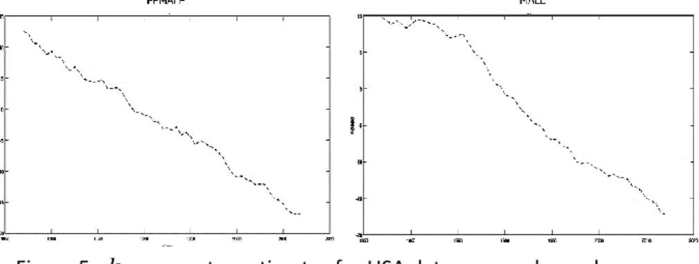
Figure 5 - 𝑘𝑡 parameter estimates for USA data per gender and year ... 24

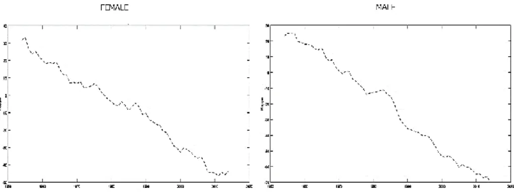
Figure 6 - 𝑘𝑡 parameter estimates for Japan data per gender and year ... 25

Figure 7 - 𝜇𝑥𝑡 values for each country and gender, per year. ... 25

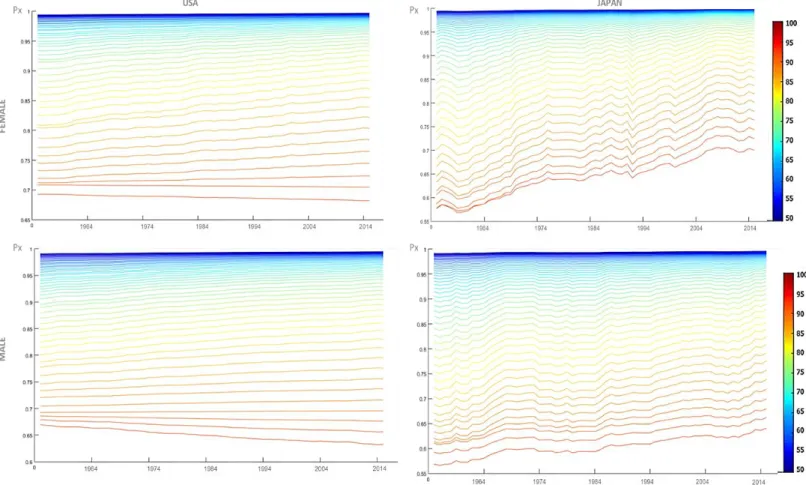
Figure 8 Survival Probabilities (𝑝𝑥, 𝑡)for USA and Japan data ... 26

Figure 9 – Female and Male premiums for 65 and 85 ages and risk level 0.1 ... 31

Figure 10 - Female and Male premiums for 65 and 85 ages and risk level 0.3 ... 32

LIST OF TABLES

Table 2 – Longevity Swap prices for different maturities and longevity risk premium levels using US Female data (2010-2014) ... 28

Table 3 – Longevity Swap prices for different maturities and longevity risk premium levels using Japan Female data (2010-2014) ... 28

Table 4- Swap Premiums for different maturities and risk using US Male data (2010-2014) . 29 Table 5 - Swap Premiums for different maturities and risk using Japan Male data (2010-2014) ... 30

7

1. INTRODUCTION

Financial theory characterizes the risk by the dispersion of expected results on a certain investment, in consequence of movements in the financial variables (risk factors). The financial risk is multidimensional and, therefore, in recent years, risk management had an ample advance. One of the risks that have grown a lot is longevity risk. We can define longevity risk as the uncertainty on projections of longevity and massive amounts of liabilities exposed to this risk (Blake et al., 2006) or simply the risk that life spans exceed expectation, resulting in individual mortality rates lower than expected (Coughlan et al., 2011).

Longevity risk can be distinguished into different dimensions as Blake et al. (p.506, 2013) mentioned: (i) micro-longevity risk or non-systematic risk; (ii) macro-longevity risk or systematic risk. Macro-longevity risk refers to the longevity risk in a huge group of people, such as members of a large pension plan or the annuitants in the annuity book of a large insurer. On macro-longevity risk, the trend risk is an example of a systematic or aggregative risk. The micro-longevity risk is the opposite, deals with the longevity risk in a small group of individuals, such as those underlying a life settlement fund, for example, an investment on individual life assurance policies. In this paper, the main concept will be macro-longevity risk, since this is the most critical dimension of the global economy and the sustainability of insurance sector.

The noticeable growth of scientific research about longevity risk and how to model it is flagrant in the last decades, partly due to the embryonic work of Lee and Carter (1992). The fact that longevity risk has become a major focus of scientific research is explained by several reasons, one of them is its importance in developed societies. The longevity caused by the considerable changes in the lives and welfare of the developed countries took substantial fluctuations on the demographic transitions and had profound effects on the size, age, and structure of the world population. In developed countries, before 1900, the world population growth was slow, the age structure remained practically constant and relatively few people lived beyond 65 years. During the first half of the twentieth century, they began to draw up new rates of life expectancy, together with population growth. During the second half of the twentieth century this scenario has changed: fertility rates declined to almost half causing the slowdown in population growth, the percentage of young people in age pyramids began to lose to the older players, and aging population began to be a reality, increasingly apparent and sharp (Batini, Callen & McKibbin, 2006). Demographic changes reached all countries of the world not only developed countries, although these countries unfold at different rates. The economic and financial impact of demographic transitions is highlighted in Batini, Callen & Mckibbin (2006), where the percentage differences in the growth of countries would be between 30% to 60% lower. Differences in demographic transitions and the singularities of their indicators allow investors to understand the longevity risk, observe the movement of the indicators in the various angles of the world, to understand and predict potential longevity

8

shocks over time and uncover new forms and products to cover them (Creighton, Jin, Piggott, & Valdez, 2005; Nakada et al., 2014).

However, the impact of global demographic changes, particularly those that took place in most developed countries, has brought new challenges to the insurance sector, its sustainability, as well as challenges to the economy itself. These difficulties are also a reason for the increasing scientific contribution in this area. Boyer and Stentoft (2013, pp. 35) mentioned that “(…)the longevity affected the overall profitability of institutions that offer lifetime pensions, such as large corporations and governments, as well the total savings of the individuals”. This happened because the insurance companies could not turn the mortality probability profitable enough through the large numbers rule, due the exponential increase of life expectancy in all the corners of the world.

According to Dowd et al. (2006) if people live longer than anticipated, insurance companies make losses on their annuity books; and if people die sooner than projected, companies make losses on their life books. Due to this, it is important that insurance companies keep an appropriate reserve level to cover such eventualities, always preserving their solvency. The problem with this approach is that capital is costly and, given the difficulties of forecasting mortality rates over even short time horizons, it is hard to determine what adequate capital levels might be. Due to these situations, the insurance and reinsurance market (the traditional markets used to trade longevity risk products) have become insufficient, not because this type of risk was not manageable for insurance companies, but, due the exponential increase of life expectancy, longevity became difficult to commercialize through profitable products for insurance companies (even with reinsurers) and low-cost level for consumers. While the insurance sector was facing difficult challenges to manage longevity risk, the derivatives markets were growing exponentially to hedging the various types of risks. This growth of derivatives has become another reason that pushed longevity risk research forward, taking into consideration the potentialities and possible combinations between two separate “worlds” – insurance traditional life risk and capital markets instruments.

The academic community, considering the size of the risk exposure, pointed the only way to potentially manage longevity risk by drawing upon the wealth of the entire capital market (Boyer and Stentoft, 2013). Then this solution came in 2008 when the world saw the first capital markets solutions for longevity risk, in a deal between Lucida ple and Canada Life in the United Kingdom (Coughlan et al., 2011). These two transactions made possible the development of the longevity risk transfer market, bringing additional capacity, flexibility, and transparency to complement existing insurance solutions that were insufficient. According to Boyer and Stentoft (2013 p.36), “The ability of capital markets to absorb larger amounts of risk than the market for life reinsurance stems from two factors: (i) first, capital markets are huge and much greater than the market capitalization and surplus of the insurance industry; (ii) second, there is virtually no correlation between longevity risk and market risk so that exposure to longevity risk shifts the portfolio frontier up and to the left”.

9

However, the development of capital market solutions for longevity risk has been too slow. Despite the capacity of financial markets to absorb this type of risk, some instruments have many challenges on the calculation of their fair values. The main challenges are: (i) first, mortality is not a traded asset and therefore we cannot value longevity products using non-arbitrage principles, since we cannot build a replication portfolio; (ii) second, given that the cash flows of these products are directly linked to mortality or survival rates, their valuation requires the ability to forecast these rates accurately (Boyer and Stentof, 2013 p.36). On the other hand, the economic relevance/global exposure of the insurance sector is too high to let this system collapse. It is thus necessary to develop new techniques for computing the fair value of capital markets solutions to longevity risk to answer the demands of collective needs, since the number of institutions is “short” longevity, i.e., their liabilities increase if longevity increases.

Taking into consideration the importance of longevity risk in developed societies, the insufficiency of insurance sector solutions to absorb this risk and the capital market potentiality’s, the goal of this paper is to price a Longevity Swap using the risk-neutral simulation approach developed by Boyer and Stentoft (2013), assuming the dynamics of mortality rates is modelled using log bilinear Lee-Carter model under a Poisson setting, and the risk-neutral distribution of the innovations is obtained using the Wang transform. Taking this goal into account, in this paper we forecast the force of mortality using the log-bilinear Lee-Carter model under a Poisson setting to compare the survival probabilities of the female and male populations of the USA and Japan. We then compute longevity Swap premiums (taking into consideration both, USA and Japan data, for the different genders and ages) applying a risk-neutral simulated method for pricing.

This paper contributes to the growing literature debate on the need for manage longevity/ mortality risk in the insurance and pension fund industries. This will be done through two different ways, the first one is the claim that cross-country capital markets can absorb the longevity risk, being a profitable tool; and the second, is in demonstrating that swaps can be an effective hedging and trading instrument for the major risks in the XXI century, surpassing the difficulties of their fair value calculations. To answer this main goal, the paper is split into three logical sections; the first section makes a review of the research done regarding capital markets solutions to hedge longevity risk, with more detail on longevity swaps. The second section describes the methodology of risk-neutral simulation and how this method will be applied in this paper. Finally, we conduct an empirical investigation on how to price the longevity vanilla swap using USA and Japan data (exploring female and male mortality data in separate scenarios) using the risk neutral simulation approach.

10

2. LONGEVITY RISK SOLUTIONS: TRADITIONAL AND DERIVATIVES PRODUCTS

Longevity risk is the risk that life spans exceed expectation, resulting in individual mortality rates lower than expected. This type of risk is one of the most relevant risks to the economy, due to the importance and the consequences of longevity in our days. Longevity becomes a key concept discussed in the XXI century, due to the multiple demographic changes felt in almost all the countries of the world (developed and developing countries). The technological revolution at medical, agriculture and industrial levels allowed populations to live longer than anticipated and challenging the economic sustainability every day. One example of the current challenges faced by insurance companies is the difficulty in profiting from traditional longevity insurance products due to both longevity and interest rate risks. Due to these incapacities, derivatives become the key focus for hedging longevity risk. Below, we describe how longevity could be hedge with traditional and derivatives products through a brief literature review.

2.1 LONGEVITY TRADITIONAL PRODUCTS

Until the XXI century longevity risk was hedged by insurance companies through conventional and conservative methods. The traditional solutions to hedge this type of risk had itself an evolution, from basic methods to “advanced” forms.

Blake, Cairns & Dowd (2006) claim that insurance companies started to respond to longevity risk by simply accepting the risk as part of their core business, which they understand well and are used to manage. After, they began to share longevity risk across distinct types of products, socio-economic groups and countries, this way they could balance their portfolios by seeking to exploit the conceivable natural hedges involved running a mixed business of term assurance and annuity.

However, since longevity became difficult to hedge due its significant exposure, insurance companies required another type of guarantee to make this risk manageable and sustainable. Due to this, the various forms of reinsure with a reinsuring company have become the answer to hedge longevity, since those contracts allowed sharing some, or all, of the downside of longevity risk with the reinsurer.

Besides reinsurance, pension plans allowed arrange for a bulk buyout of their pensions in payment, passing on the responsibility for payment to an insurance company, permitted risk sharing as reinsurance contracts. Similarly, smaller pension plans are accustomed to purchasing annuities at the time of retirement for each plan member. This hedges the total risk in their pool of pensioners. Unless the plan purchases deferred pensions on a regular basis, it still bears the longevity risk for current active members and deferred pensioners between now and their retirement dates (by Blake, Cairns & Dowd, 2006).

11

Insurance companies which are annuity providers might choose to replace the traditional non-participating annuities for non-participating contracts. These contracts allow passing part of the exposure to longevity risk to the surviving participating policyholders, this way the companies can hedge the risk more easily, since those products that pay bonuses or survival credits to annuitants that can take account of experienced mortality rates within the pool of annuitants. Nonetheless, since the cost of reinsurance is high, pensions and annuity provided only applied it to a limited extent, the securitization on mortality starting to appear - since the need to trade longevity risk at a low cost was a priority (Cowley & Cummins, 2005).

The traditional longevity risk solutions described above began collapsing due to their insufficiencies to address the risk at low hedging costs on a large group of people that live longer than expected. As a result, insurance companies and pension plans started to manage longevity risk using mortality-linked securities on traded contacts such as longevity bonds, annuity futures, forwards, index-based instruments and, finally, swaps and options. These institutions began transferring risk to the only entity that can manage these exposure amounts: capital market (Dowd et al., 2006). The capital market was and still is, the only solution to respond to a significant number of collective needs of the users, suppressing the short number and the capacity of the institutions that trade/manage mortality risk. Below we describe these new instruments.

2.2 LONGEVITY DERIVATIVE PRODUCTS

The derivative products for longevity emerged as an obvious solution to trade and deal with higher amounts of exposures, crushing the advantages of the traditional solutions to manage longevity or mortality risk. Derivatives for longevity were launched in different generations/ steps of time. Fung et al. (2005) classified the capital markets solutions for longevity risk in three different generations: (i) the first generation was based on longevity/survival bonds; (ii) followed by q-forwards, survival/mortality futures and survival/mortality swaps on second stage; (ii) and finally, longevity/survival options. These securities have the usual features we would expect to find in bonds, swaps, futures and options.

As mentioned by Blake, Cairns & Dowd (2006), there is an important distinction between those that are traded over-the-counter markets (OTC) (e.g. swaps), and those that are traded on organised exchanges (e.g. futures); and those who have a linear payoff with the one's with non-linear payoff. The former has the attraction that they can be tailor-made to the requirements of a user (which keeps down basis risk), but have the disadvantage that they have thin secondary markets (which makes positions harder to unwind); the latter has the attraction of greater market liquidity (which facilitates unwinding), but have the disadvantage of increased basis risk.

12

The first generation of capital market solutions was based on bonds, longevity bonds, the most basic instrument to hedge the risk (Blake & Burrows, 2001; Blake et al., 2006a; Bauer et al.,2010; Fung et. all, 2015). In the literature, we found different types of bonds that trade longevity. Blake, Cairns & Dowd (2006) distinguish two main types of bonds: (i) the first are “principal-at-risk” longevity bonds (longevity bonds in which the investor risks losing all or part of the principal if the relevant mortality event occurs); (ii) the second are “coupon-based” longevity bonds (these are bonds in which the coupon-payment is mortality-dependent). The nature of this dependence can also vary: the payment might be a smooth function of a mortality index, or it might be specified in ‘at risk’ terms, i.e. the investor loses some or the entire coupon if the mortality index crosses some threshold. Coupon-based bonds are distinguished in many types: (i) the classical longevity bonds; (ii) the zero-coupon bonds, the (iii) deferred longevity bonds and (iv) other kinds. Besides these two categories, we can also have an array of more complex hybrid longevity bonds.

The “principal-at-risk” longevity bond became popular through the Swiss Re mortality bond in 2003. This bond helped to reduce Swiss Re's exposure to a catastrophic mortality deterioration. The structure of this bond is simple, as explained in Blake et al. (2006). The bond is issued by a single pension plan or annuity provider (A) using a special purpose vehicle (SPV). At the outset, the SPV is funded by contributions from A and external investors (B). The total outgo of the SPV would mimic either a floating-rate or a fixed interest bond paying annual coupons and with a final repayment of principal at maturity. Under normal circumstances coupons and principal would be payable in full to B. However, if a designated survival index, S(t), exceeds a specified threshold then a reduction in the repayment of principal to B (and possibly also the coupons) would be triggered, with the residual payable to A Blake, Cairns & Dowd, 2006).

On the other hand, the “coupon-based” longevity bond become popular trough EIB/ BNPP transaction. This bond commercialized with the European Investment Bank (EIB) in 2004, which was underwritten by BNP Paribas – as the designer and originator and Partner Re as the longevity risk reinsurer. The face value of the issue was £540 million, and the bond had a 25-year maturity. The bond was an annuity (or amortizing) bond with floating coupon payments, and its innovative feature was to link the coupon payments to a cohort survival index based on the realized mortality rates of English and Welsh males aged 65 in 2002. This bond worked like a classic longevity bond (Blake et al., 2006).

However, although an innovation, this bond generation had limited success, wasn’t well received by investors, and couldn’t generate enough demand to be launched due to its deficiencies, but was crucial to present the longevity products on capital markets due the public attention received.

Like the first generation, the second involved linear payoff instruments, but in this time most complex contracts were used: forwards, futures and swaps. Q-forwards launched this

13

generation, the mortality hedge was provided by J.P Morgan, and was novel not just because it involved a longevity index and a new kind of product, but also because it was a hedge of value rather than a hedge of cash payments. The importance of q-forwards rests on the fact that they form basic blocks from which other, complex, life-related derivatives can be constructed. When appropriately designed, a portfolio of q-forwards can be used to replicate and to hedge the longevity exposure of an annuity or a pension liability or to hedge the mortality exposures of a life assurance book.

As mentioned by Black et al. (2003), a q-forward is similar to a forward contract, however, uses mortality as an asset. It is defined as an agreement between two parties in which they agree to exchange an amount proportional to the actual, realized mortality rate of a given population (or subpopulation) in return for an amount proportional to a fixed mortality rate that has been mutually agreed at inception to be payable at a future date (the maturity of the contract). In this sense, a q-forward is a swap that exchanges fixed mortality for the realized mortality at maturity. As for the other derivative products, the variable used to settle the contract is the realized mortality rate for the reference population in a future period. In short hedging longevity risk in a pension plan, using a q-forward the pension plan will receive the fixed mortality rate and pay the realized mortality rate (and hence locks in the future mortality rate it should pay whatever happens to actual rates). The counterparty to this transaction, typically an investment bank, has the different exposure, paying the fixed mortality rates, and receiving the realized rate.

Due to q-forward success, another type of contracts started to be envisaged: futures and swaps. Futures on longevity are very like the q-forwards, instruments to hedge longevity risk. However, this type of contracts is more inflexible than q-forwards, since the last ones are customized (Barrieu, Veraart, 2014; LIMA, 2010a). In short, the basic form of a futures contract involves defining the underlying (typically price) process, S(t), that will define the payoff in the future, and the delivery date, T, of the futures contract, mortality futures follow this logic (Blake, Cairns & Dowd, 2006). Many studies showed the potentialities of futures markets (see Gray, 1978, Ederington, 1979, Carlton, 1984, Black, 1986, Pierog & Stein,1989, Corkish, Holland & Vila, 1997 and Brorsen & Fofana, 2001). However, mortality futures had and still have, some difficulties in establishing a longevity market. If a liquid market in longevity bonds develops in time, then it might be possible for a futures market to develop which uses the price or prices of longevity bonds as the underlying (Blake, Cairns & Dowd, 2006).

Contrary to futures, longevity swap contracts became a considerable success story. The first longevity swap transaction was recorded by J.P. Morgan in July 2008, with Canada Life in the United Kingdom (Blacke et al., 2013). It was a 40-year maturity £500 million longevity swap that was linked not to an index, but to the actual mortality experience of the 125.000-plus annuitants in the annuity portfolio that was being hedged. It also differed in being a cash flow hedge of longevity risk. But, most significantly, this transaction brought capital markets investors into the Life Market for the very first time, as the longevity risk was passed from

14

Canada Life to J.P. Morgan and then directly on to investors. This has become the archetypal longevity swap upon which other transactions are based (Blake et al., 2013).

A longevity swap is as an instrument that involves exchanging actual pension payments for a series of pre-agreed fixed payments. Each payment is based on an amount-weighed survival rate. After this transaction, longevity swaps (or survival swaps) became a big focus on capital markets solutions to hedge longevity risk, due to its multiple advantages. This second generation caught much more attraction from investors due to its ability to manage appropriately systematic mortality risk, particularly index-based longevity swaps that can be traded as standardized contracts, and due to their lower hedging costs.

Finally, the last generation of capital markets instruments solutions is based on options, non-linear payoff instruments. As claimed by Blake, Cairns & Dowd (2006), it's possible to have a lot of assorted products in this generation, such as (i) survival caps; (ii) survival floors; (iii) annuity futures options; (iv) OTC options and embedded options; and more complex products such as (v) mortality swaptions. Non-linear derivatives for longevity risk are still a solution not well explored and accepted by investors, due to the inherent risks that they carry (Fung et al., 2015; Bayer et al., 2010).

The focus of this article is on second generation instruments, due the growing attention in these products. More specifically, longevity swaps will be the derivative product use to show an effective tool to hedge longevity risk. In the sub-section below we will present in more detail the longevity swaps as well as ways to price this tool.

2.2.1 LONGEVITY/SURVIVAL SWAPS

As mentioned in the previous section, longevity swaps are one of considerable success of capital markets second generation solutions, due to their attractive intrinsic characteristics. The first mortality swap showed in the market was the one embedded in the EIB bond, mentioned in the section above. A swap for mortality issues has some advantages when compared with others capital markets solutions. Like referred by Blake et al., (2006, p.19), swaps can be arranged at lower transactions cost than a bond and are more easily cancelled. They are more flexible than other solutions and can be tailor-made to suit diverse circumstances. They do not require the existence of a liquid market, just the willingness of counterparties to exploit their comparative advantages or trade views on the development of mortality over time. A swap also has advantages over traditional insurance arrangements: they involve lower transactions costs and are more flexible than reinsurance treaties, due to the fact of that instruments aren’t insurance contracts in the legal sense of the term, so aren’t affected by legal features like indemnity, insurable interest etc. Instead are subjective instruments, in terms of requirements of securities law, so it is allowed to speculate on a random variable and does not required the policyholder to have an insurable interest.

15

Because of these advantages, it's known from industry contracts that some insurance companies have already entered mortality or longevity swaps on OTC (over-the-counter) basis. The counterparties are usually life companies, and some investment banks are also interested in swap transactions. The attractions of these agreements are obvious ones of risk mitigation and capital release for those laying off longevity risk, and low-beta risk exposures for those taking it on (Blake, Cairns & Dowd, 2006, p.20).

As Cox & Lin (2004) explained, a mortality swap can also be used to help firms that run both annuity and life books to manage the natural hedges implicit in their positions. The type of swap, in this case, might be a floating- for-floating swap, with one floating leg tied to the annuity provider's annuity payments and the other to the life assurer's insurance pay-outs (Blake et al., 2006). Swaps can also be used as vehicles to speculate on longevity risk, so it’s a type of contract that pleases all parties in the capital markets.

Despite its advantages, a swap is a risk management tool and is therefore subject to certain kinds of risk. The main risk that one longevity swap can have for the buyers is counterparty risk. This is a major problem with most swaps because swaps can entail significant exposures to counterparty credit risk. One straightforward way to upgrade these respective counterparty risks is for the swap to specify that payments are to be made on a net rather than gross basis, which is why existing swaps routinely specify net payment (Dowd et al., 2006). Achieving further reductions in counterparty exposure is more difficult, but such problems are common to OTC derivatives trades, and the standard methods of dealing with them in OTC derivatives markets could also be used to handle counterparty credit issues in survival or longevity swaps markets as well, like mentioned by Dowd et al. (2006) special purpose vehicles, credit insurance and credit derivatives and credit enhancement.

In the literature, the longevity and survival swaps are addressed by diverse authors, especially, by Dawson (2002), Blake (2003), Dowd (2003), Dawson (2006), Blake et al., (2006) and Lin and Cox (2005). In terms of definitions, mortality-linked swaps are divided into two distinct types, depending on the underlying asset: (i) Mortality Swaps or (ii) Longevity/Survival Swaps. Both instruments originated in capital markets to hedge longevity risk, however, although they have similar characteristics, each one provides a hedge for different risk factor: mortality (demise early than expected) or longevity (live longer than anticipated). In this paper, our focus will be longevity/survival swaps as defined by Dowd et al. (2006).

Besides this basic distinction, a swap can have diverse types: (i) it can be a standardized hedge, or a (ii) customized hedge. As Blake et al. (2013) described, a standardized index-based longevity swap hedges have some advantages over the customized hedges in terms of simplicity, cost and liquidity. But they also have obvious disadvantages, principally the fact that they are not perfect hedges and leave a residual basis risk that requires the index hedge to be carefully calibrated. Contrary, customized hedges are custom-made, so they’ have an exact hedge (so no residual basis risk’s), however, are poor in liquidity, expensive and have

16

longer maturities than the standardized (more counterparty credit exposure) so are less attractive to investors.

In the most basic case, a swap, for distinct types of hedges (customized or standardized) and underlying asset (mortality or longevity), are defined as an agreement by which two parties agree to exchange one or more future cash flows, at least one of which is random (Dowd et al., 2006). Taking into consideration a definition of swap, one longevity swap could be defined as an agreement to exchange one or more cash flows in the future based on the outcome of at least one (random) longevity-dependent payment (Blake et al., 2006 p.19).

A variety of swaps that trade longevity/mortality as an underlying asset can be found in scientific papers, from the most basic forms like (i) one-payment mortality (or survival) swaps; (ii) vanilla mortality (or survival) swaps, up to other more complex forms like: (i) swaps on mortality spreads; (ii) cross-currency mortality swaps; (iii) mortality swaps in which one or more floating payment depends on a non-mortality random variable (for example an interest rate, a stock index, etc.); and (iv) mortality swaps with embedded features such as options (Blake, Cairns & Dowd, 2006 p.21).

One-payment mortality (or survival) swap is the most basic form of swaps on longevity and mortality business, involve exchange, at time 0, of a single payment K(t), for a single random mortality-dependent payment S(t) at some future time t (Blake et al., 2006 p.19). On the other hand, the vanilla survival or longevity swap is a swap in which the parties agree to swap a series of payments periodically (i.e., for every t = 1, 2, . . . , T) until the swap matures in period T (Dowd et al. 2006). This type of swap is reminiscent of a vanilla interest-rate swap (IRS), which involves one fixed leg and one floating leg typically related to a market rate such as LIBOR/EURIBOR. However, like mentioned by Dowd (2006 p.4), there are several key differences: (i) the fixed leg of the IRS specifies payments that are constant over time, whereas the corresponding leg of the Vanilla Survivor Swaps (VSS) involves present payments that decline over time in line with the survival index anticipated at time 0; (ii) also, the floating leg of the IRS is tied to a market interest rate, whereas the floating leg of the VSS depends on the realized value of the survival index at time t; (iii) finally, the IRS can be valued using a zero-arbitrage condition because of the existence of a liquid bond market.

This is not the case with a VSS which must be valued in incomplete markets setting. Besides these two types, we could have swaps that involve the exchange of one floating-rate payment for another or more elaborate types of swap: swaps on mortality spreads, cross-currency mortality swaps, mortality swaps in which one or more floating payment depends on a non-mortality random variable (an interest rate, a stock index, etc.), and non-mortality swaps with embedded features such as options (Blake et al., 2006 p.21).

The swaps described above discussed and developed by various authors like Dawson (2002), Blake (2003), Dowd (2003), Dowd et al. (2006), Blake et al., (2006), Cox and Lin (2004) and Lin and Cox (2005). In addition to the notable contributions in terms of definition and structure

17

of longevity and mortality swaps by Blake et al. (2006; 2013; 2003) and Dowd et al. (2006;2003) in their vast portfolio of articles, Lin and Cox (2004;2005) had one of the most significant contributions to the subject. These two authors present survival/longevity swaps as ideal instruments for managing, hedging, and trading mortality-dependent risks, and they offer many benefits to insurance companies that need to manage such risks, besides that, they show how swaps can be priced, and provide a thorough analysis of how insurance companies might use them to exploit natural hedge opportunities across their annuity and life businesses. In this paper we will be using a vanilla longevity swap to hedge the longevity risk for USA and Japan. Like Boyer and Stentoft (2003), on this vanilla longevity swap, the premium of this swap is one simple portfolio of q-forwards, since a q-forward is the easiest instrument which can be used to hedge the exposures to longevity risk at a given moment, and but extension a portfolio of such forwards can be used to hedge the risk over a period. This type of instrument is well known in the market for interest rate risk where the combined portfolio is traded together as an interest rate swap. So, similarly a survival or longevity swap is the simplest one portfolio of q-forwards. To better understand how this type of swap works let’s analyse the q-forwards math. Following Boyer and Stentoft (2003), to illustrate how a q-forward works let Sx,t e be the expected probability that an individual aged x survives from time t-1 to time t, give the information currently available. Similarly, let S_x,t r be the realized percentage of individuals aged x that survive from time t-1 to time 1. Knowing that a forward premium today is then fixed such that:

NPV (adjusted fixed leg) = NPV (floating leg)

(1)

And defined the adjustment factor πf_{t of this q-}f_{orward as the solution to:}

(1 + 𝜋_𝑡 𝑓)𝑁𝑃𝑉 (𝑆𝑥,𝑡 𝑒 ) = 𝑁𝑃𝑉 (𝑆𝑥,𝑡 𝑟 )

(2)

Besides the fixed amount being dependent on the expected survival rate, these are conditional information at the time of pricing and hence know and fixed, we can calculate πf_t as follows:

18

(𝜋

) =

𝑟 ₎

𝑁𝑃𝑉 (𝑆_𝑥,𝑡 𝑒 )

− 1

(3)

Where the result is the price of the q-forward at this moment. When we have a contract with different maturities, for example, the premium for one q-forward contract on the survival rates from time t to t+1 the price will be:

(𝜋_𝑡+1 𝑓 ) =𝑁𝑃𝑉 (𝑆𝑥,𝑡+1

𝑟 ₎

𝑁𝑃𝑉 (𝑆_𝑥,𝑡+1 𝑒 )− 1

(4)

Knowing the price of a q-forward, it’s easier to understand the price of one longevity swap since it’s a simple portfolio of q-forwards. For example, we could consider a swap on the survival rates from t−1 to t, from t to t + 1, and from t + 1 to t + 2. The straightforward generalization of the formula for the q-forward price formula showed yields the following solution for the longevity swap price:

(𝜋_𝑡,𝑡+2𝑆 ) = 𝑁𝑃𝑉 (𝑆𝑥,𝑡

𝑟 _{) + 𝑁𝑃𝑉 (𝑆}

𝑥,𝑡+1 𝑟 ) + 𝑁𝑃𝑉 (𝑆𝑥,𝑡+2 𝑟 )

𝑁𝑃𝑉 (𝑆_𝑥,𝑡+1 𝑒 ) + 𝑁𝑃𝑉 (𝑆_{𝑥,𝑡+1+1} 𝑒 ) + 𝑁𝑃𝑉 (𝑆_𝑥,𝑡+2 𝑒 )− 1

(5)

Thus, the net payment to a long position in this swap, at time t, is given by the expression below, where these payments are realized until the end of the contract:

𝑆_𝑥,𝑡 𝑟 − (1 + 𝜋_𝑡,𝑡+2𝑆 ) 𝑆_𝑥,𝑡 𝑒

(6)

In this article, we’ll consider the mortality of different ages across the time and structure longevity derivatives directly on a given survival probabilities.

19

2. HOW TO PRICE DERIVATIVES USING SIMULATION

3.1. NEUTRAL RISK DISTRIBUTIONS

In literature, alternative approaches for pricing longevity-linked derivatives have been presented. These instruments require the ability to forecast future mortality rates. Some studies use mortality projection models, such as extrapolation models. However, we can be pricing derivatives follow a derivative pricing perspective, using risk-neutral simulation technique.

Boyer and Stentoft (2013) showed how risk-neutral distributions and risk-neutral simulation could be used to evaluate derivate products, such as forwards, swaps and options. In this paper, we’ll follow this methodology since it is a type of approach which surpasses some difficulties to evaluate the derivatives based on mortality (the reason that has in part delayed the development of this market).

In longevity-derivative products, mortality or longevity are traded like another type of underlying asset. However, mortality or longevity are not continuously traded assets and as such, this market is to be considered incomplete and a risk premium exists for the exposure to this type of risky asset (Boyer and Stentoft, 2013). Wang (2000) and Boyer and Stentoft, 2013) showed how to evaluate a financial asset basing on a distortion of the cumulative distribution of a variable X. This yields a new risk-adjusted cumulative distribution of cash flows that can then be discounted at the free rate. Wang (2000) defines the following risk-adjusted distribution:

𝐹 ̃ (𝑥) = Φ [Φ−1 _{(𝐹(𝑥)) − 𝜆 ],}

(7)

where:

• 𝐹 ̃ (𝑥) is the cumulative distribution function of variable X • Φ is the normal cumulative distribution function

• 𝜆 is a risk premium

With the Wang-distortion above, it is possible to price derivatives easily, since this method can be applied to any type of distribution function F (x) and can be adjusted to account for the uncertainty (the risk) that surrounds the distribution parameters. This distortion retains the so desirable normal and Log-Normal distributions. So, if X follows a Normal distribution with N (μ, σ2) then the transformed variable X̃ also follows a normal distribution with N (μ − λσ, σ2); following the same thought, if X follows a Log- Normal distribution with ln(X)~ N (μ, σ2_{), then the transformed variable X̃ also follows a Log-Normal distribution with} ln(X̃ )~ N (μ − λσ, σ2_{). Due this, this transformation has a lot of advantages for pricing the} derivatives.

20

3.2. RISK NEUTRAL SIMULATION

Using the Wang-distortion above, it is possible distort the final distribution including the risk premium (λ), which adjust the calculations due to the risk and allows to obtain the price of the swap contract. To apply this method, it is necessary to adjust the risk directly to the simulation, by the method used through Boyer and Stentoft (2013) research, the risk neutral simulation approach. The risk neutral simulation has an immediate benefit since all paths have equal probability to occur. This method is applied thought the property of the Normal and Log-Normal models mentioned in previous section. In particular, since the distortion retains the Normal and Log-Normal distributions, an obvious alternative to the method of risk adjusting the distribution is to simulate directly the risk adjusted innovations. In a Normal model for example, we simulate directly with innovations that are ϵ~ N(− λσ, σ2) instead a ϵ~ N(0, σ2_{) and then distorting the distribution according the risk (Boyer and Stentoft, 2013).}

3.3. STOCHASTIC MODELING AND CALIBRATION: MORTALITY PARAMETERS AND PROBABILITIES CALCULATION

As mentioned above, the biggest problem in pricing longevity derivatives are mortality rates, since they are very difficult to predict. For forecasting futures mortality rates, various stochastic models have been developed. The first contribution to a prediction of dynamic mortality was a proposal by Blaschke (1923) who introduced a version based on Makeham's law. However, only later, with the work of Lee & Carter (1992), we have made significant progress in the stochastic modelling of mortality. Using the central mortality rates of the United States of America, the authors presented an extrapolation model that allows, in a simple way, to describe a mortality of the population using a single time trend parameter, projected using time series methods.

Other authors also sought to introduce improvements in the formulation of Lee-Carter, especially Wilmoth (1993), Alho (2000), Brouhns et al. (2002) and Renshaw & Haberman (2006), that introduced some improvements on Lee-Carter model using a log-bilinear Poisson regression to estimate the parameters, instead of using the principal components decomposition method (which presents problems of homoscedasticity). Renshaw & Haberman (2008) provide an extension of the Lee-Carter model that allows for the inclusion of cohort effects, that is, it is a year of birth. Years later, Cairns et al. (2006) introduced a similar model called CBD (Cairns-Blake-Dowd), which contains two stochastic factors to represent the mortality dynamics.

In this article, we’ll provide results for the case when the dynamic of mortality rates is modelled using the log-bilinear Lee-Carter model under a Poisson setting. To better understand this model we’ll describe briefly the Lee-Carter-Poisson model used.

21

The log-bilinear Poisson Lee-Carter model assumes the following:

𝐷_𝑥,𝑡 ~ 𝑃𝑜𝑖𝑠𝑠𝑜𝑛 (𝜇_𝑥(𝑡)𝐸_𝑥,𝑡) 𝑤𝑖𝑡ℎ 𝜇_𝑥(𝑡) = 𝑒𝛼𝑥+ 𝛽𝑥 𝐾𝑡

(8)

Where:

• 𝜇𝑥(𝑡) is the observed force of mortality at age 𝑥 during the year t;

• 𝐷_𝑥,𝑡 is the number of deaths recorded at age 𝑥 during the year t, from those exposed-to-risk 𝐸𝑥,𝑡

• 𝛼_𝑥 denotes the general shape of the mortality schedule • 𝛽𝑥 represents the age-specific patterns of mortality change • 𝑘_𝑡 represents the time trend

To forecast the mortality rates, we calibrate this model to the USA and Japan population (male and female), using data from 1954 to 2014 and ages 50-100 for estimation. Data on deaths and risk exposures are obtained from the Human Mortality Database. The parameter estimates are obtained using Linear Models and an interactive method for estimation log-bilinear as Goodman (1979). Goodman iterative process takes advantage of the Newton-Raphson algorithm to estimate the mortality parameters with log-bilinear parameters. In general terms, this iterative process involves using, in each iteration (v + 1), a set of parameters θ = (θ1, θ2, … . , θn), while the other parameters remain fixed, using:

𝜃̂(𝑣+1) = 𝜃̂(𝑣)− 𝜕𝐿(𝑣) 𝜕𝜃 𝜕2_𝐿(𝑣) 𝜕𝜃2 where 𝐿(𝑣) = 𝐿(𝑣) (𝜃̂(𝑣))

(9)

To implement this algorithm, we follow Brouhns et al. (2002) steps to estimate the mortality parameters (αx, βx, kx), where the updating scheme follows the below itineration’s, starting with α̂_x(0) = 0, β̂_x(0) = 1, k̂_t(0)= 0: 𝛼̂_𝑥(𝑣+1)= 𝛼̂_𝑥(𝑣)− ∑ (𝐷𝑥𝑡− 𝐷̂𝑥𝑡 (𝑣) 𝑡 ) − ∑ 𝐷̂ 𝑥𝑡 (𝑣) 𝑡 , 𝛽̂_𝑥(𝑣+1) = 𝛽̂_𝑥(𝑣), 𝑘̂_𝑡(𝑣+1)= 𝑘_𝑡(𝑣) 𝑘̂_𝑥(𝑣+2)= 𝑘̂_𝑡(𝑣)− ∑ (𝐷𝑥𝑡− 𝐷̂𝑥𝑡 (𝑣+1) 𝑥 )𝛽̂𝑥 (𝑣+1) − ∑ 𝐷_𝑡̂_𝑥𝑡(𝑣+1) (𝛽̂_𝑥(𝑣+1))2 , 𝛼̂𝑥 (𝑣+2) = 𝛼̂_𝑥(𝑣+1), 𝛽̂_𝑥(𝑣+2)= 𝛽̂_𝑥(𝑣+1)

(10)

22 𝛽̂_𝑥(𝑣+3)= 𝛽̂_𝑥(𝑣+2)− ∑ (𝐷𝑥𝑡− 𝐷̂𝑥𝑡 (𝑣+2) 𝑡 )𝑘̂𝑡 (𝑣+2) − ∑ 𝐷_𝑡̂_𝑥𝑡(𝑣+2) (𝑘̂_𝑡(𝑣+2))2 , 𝛼̂𝑥 (𝑣+3) = 𝛼̂_𝑥(𝑣+2), 𝑘̂_𝑡(𝑣+3)= 𝑘̂_𝑡(𝑣+2) Where: 𝐷̂_𝑥𝑡(𝑣)= 𝐸_𝑥𝑡 𝑒(𝛼̂(𝑣)𝑥 + 𝛽̂𝑥(𝑣) 𝑘̂𝑡(𝑣))

After 1000 iterations we normalize the parameters to fulfil the Lee-Carter constraints:

𝛼̂ ← 𝛼̂ + 𝛽_𝑥 ̂ 𝑘̅ _𝑥 𝑘̂ ← (𝑘_𝑡 ̂ − 𝑘̅ ) ∑ 𝛽_𝑡 ̂ _𝑥

𝛽̂ ← _𝑥 𝛽̂𝑥

∑ 𝛽̂_𝑥 (11)

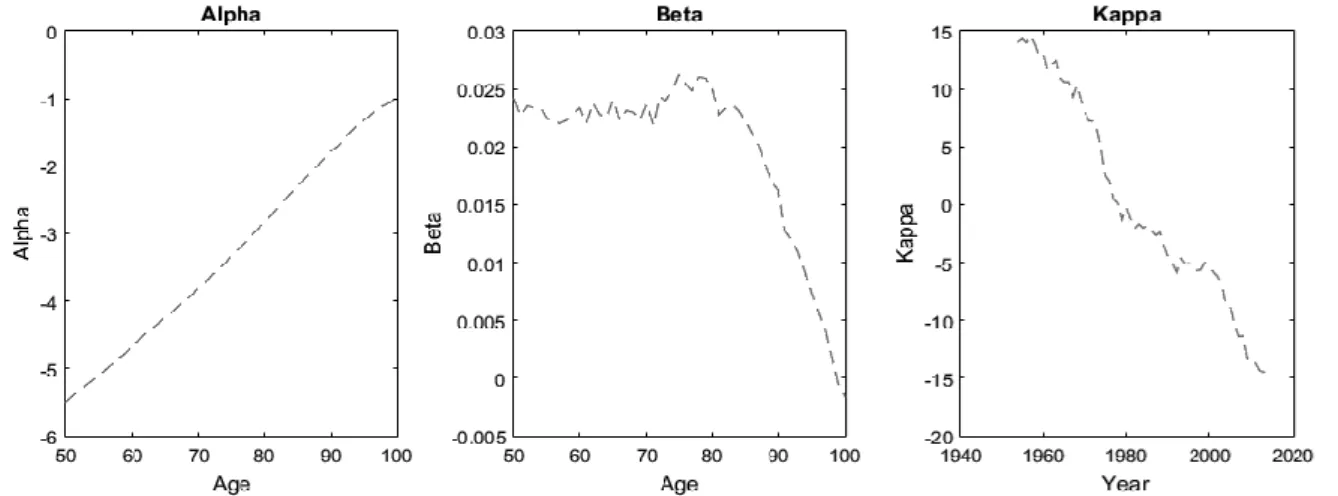
In the figures below it’s possible to see the distributions of this parameter for EUA and Japan data (female and male):

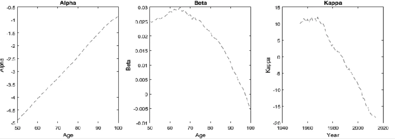
23 Figure 2 – Mortality estimator’s distribution based on USA’s male data

Figure 3 – Mortality estimator’s distribution based on Japan’s female data

24

In this model, vectors αx and βx remain constant over time and we forecast futures values of 𝑘𝑡 using a standard univariate time series model such as the classic random walk with ARIMA (0,1,0) defined as:

𝑘𝑡 = 𝜃 + 𝑘𝑡−1+ 𝜖𝑡 , 𝜖𝑡 ~𝑁(0, 𝜎2)

(12)

where the drift 𝜃 and the volatility 𝜎 are estimated from our data.

Table 1 - Parameter estimates and goodness-of-fit measures for ARIMA(0,1,0) model using data for US and Japan from 1954 to 2014.

𝜽 s.e 𝜽 𝝈𝟐 _{AIC BIC}

US Female -0.456819 0.0927076 0.559687 139.7075 141.8184 US Male -0.442613 0.085826 0.425968 123.0537 125.1646 Japan Female -1.10225 0.183781 2.24954 224.5647 226.6755 Japan Male -0.781281 0.167581 1.78297 210.3856 212.4965

The uncertainty about future mortality rates is a consequence of the uncertainty about the future values of 𝑘𝑡 as this depends critically on the innovations. For pricing, we consider the market price of longevity risk. Following the risk neutral simulation approach this is done by risk-neutralizing the innovations using the Wang distortion operator described above (Wang, 2000; Boyer and Stentoft, 2013).

So, taking advantage of the Wang-transform methodology benefits, instead of using random draws for the ϵt from a ϵ~ N(0, σ2) distribution we use draws from a ϵ~ N(− λσ, σ2) distributions, as mentioned in (12). This allows for straightforward pricing of the swap contract. Our simulation consists of N =10000 trajectories of 𝑘𝑡, to generate recursively, one of each year necessary to price the longevity derivatives, and a random Normal error, considering a given value for the risk premium parameter λ. In our simulations, we’ll use risk premium parameter between 0.0 and 0.3, range defined for Lin and Cox with reasonable estimations. In the figures below, it is possible see kt final values for each country and gender, considering λ = 0.0.

25

Figure 7 - 𝜇𝑥(𝑡) values for each country and gender, per year.

Figure 6 - 𝑘𝑡 parameter estimates for Japan data per gender and year

After all parameter estimates have been calculated, we can obtain μx(t) for each country and gender (in the figure below it is possible see this data considering λ = 0.0) and compare if the number of deaths follow the original ones, which was confirmed.

USA JAPAN FE M A LE M A LE

26

When mortality force (μx) have been calculated the survival probability (px) was obtained through the below transformation

𝑝_𝑥,𝑡 = 𝑒− 𝜇𝑥,𝑡 ₍₁₃₎

The figure below shows the survival probability for both countries and genders. As literature showed across the years, the survival probability is higher for females in both countries. However, Japan has the higher survival probability in both genders, when comparing with US data.

27

3. PRICING

LONGEVITY

SWAP

CONTRACTS:

AN

EMPIRICAL

INVESTIGATION

To compute the longevity swap premium we followed the equation below, where the survival probabilities calculated was used as the floating leg of the contract, and (NPV (Sx,t r )), and the fix leg was the mean of the calculated survival probability (NPV (Sx,t e ). We calculated the swap premiums for both genders in both countries to compare how the different genders and cultures can impact on the swap price. Beside this, we analyse the pice for different ages at initiation (65,75 and 85) and reported such simulated risk neutral density means for the years 2010-2014 and for different Wang transform's risk premium levels (λ = 0.1,0.2,0.3). This way we can analyse how the age and risk premium impact on the swap price. The notional amount used for all types of swaps is 100,000€ and a fixed risk-free rate of 3% for discounting future cash flows. The yield curve used was calculated using USA treasury department data base. The swap premiums calculations will be for different maturities (1 to 5 years).

(𝜋𝑡,𝑡+4𝑆 ) =

𝑁𝑃𝑉 (𝑆𝑥,𝑡 𝑟 ) + 𝑁𝑃𝑉 (𝑆𝑥,𝑡+1 𝑟 ) + 𝑁𝑃𝑉 (𝑆𝑥,𝑡+2 𝑟 ) + 𝑁𝑃𝑉 (𝑆𝑥,𝑡+3𝑟 ) + 𝑁𝑃𝑉 (𝑆𝑥,𝑡+4 𝑟 )

𝑁𝑃𝑉 (𝑆𝑥,𝑡+1 𝑒 ) + 𝑁𝑃𝑉 (𝑆𝑥,𝑡+1+1 𝑒 ) + 𝑁𝑃𝑉 (𝑆𝑥,𝑡+2 𝑒 ) + 𝑁𝑃𝑉 (𝑆𝑥,𝑡+3 𝑒 ) + 𝑁𝑃𝑉 (𝑆𝑥,𝑡+24𝑒 )

+ 1 (14)

Taking into consideration the information above, longevity swap premium calculation in the next section its presented for both genders, by country: (i) Female results for US and Japan data; and (ii) Male figures for US and Japan data. Please note that for both testes a sensitive analysis is done across different ages and risks levels.

3.1. TEST I – SWAP PRICING USING SURVIVAL PROBABILITIES THROUGH THE

SIMULATEDMEAN:FEMALE

Using the formula presented in (14), in the first test run, it is possible to calculate the longevity swap premiums, which are feed by female US and female Japan predicted survival probabilities (through formula 13). The results in basis points are present for US (table 1) and Japan (table 2), where it is possible to check the premiums for 1 to 5 years of maturity contracts, different ages (65, 75 and 85) and alternative longevity risk premium levels.

Analysing the premiums value from tables 2 and 3, applying a macro perspective, it is possible to check that, as the maturity increases there is an increase in the premium value, having both the same growth tendency. The same is true for the risk premium level, since as the risk rises the value of swap premiums accompanies this growth. Also, it’s possible to verify that the premium values are not identical for all ages, since for 65 years the swap premium value registers a smaller amount when compared to that of a contract designed for and individuals aged 85 years old at initiation. These tendencies follow an expected survival framework and are observable in both countries, since when the age increase the survival probability will be lower and the amount requested to cover that event would be higher. The same is applied for

28

the risk premium level and maturity, since when the risk and maturity are higher the investor should have a better return and the swap is more valuable.

The macro patterns are equal for both countries. However, exploring the values in detail it is possible to detect a few differences. In comparing US and Japan values it is noticeable that Japan premiums are slightly lower than US counterparts. This difference could be explained by the fact that survival probabilities are higher in Japan (check figure 8, when it is possible to see those differences visually).

Table 2 – Longevity Swap prices for different maturities and longevity risk premium levels using US Female data (2010-2014) x=65 1 2 3 4 5 𝜆 = 0.1 0.0801 0.1483 0.9042 1.5991 1.6626 𝜆 = 0.2 0.0837 0.1529 0.9119 1.6098 1.6778 𝜆 = 0.3 0.0872 0.1574 0.9193 1.6197 1.6918 x=75 1 2 3 4 5 λ= 0.1 0.1876 0.5602 0.9693 1.6877 2.7873 λ= 0.2 0.1876 0.5606 0.9692 1.6876 2.7874 𝜆 = 0.3 0.1872 0.5629 0.9688 1.6871 2.7864 x=85 1 2 3 4 5 λ= 0.1 0.8602 1.2178 2.0286 3.7557 4.8830 λ= 0.2 0.9104 1.2234 2.1915 3.7686 4.9012 λ= 0.3 1.9925 2.2175 3.0120 5.7458 6.8688

Table 3 – Longevity Swap prices for different maturities and longevity risk premium levels using Japan Female data (2010-2014)

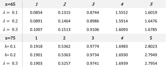
x=65 1 2 3 4 5 𝜆 = 0.1 0.0854 0.1315 0.8744 1.5552 1.6019 𝜆 = 0.2 0.0891 0.1464 0.8986 1.5914 1.6476 𝜆 = 0.3 0.1007 0.1513 0.9106 1.6093 1.6785 x=75 1 2 3 4 5 λ= 0.1 0.1918 0.5362 0.9774 1.6983 2.8023 λ= 0.2 0.1901 0.5363 0.9734 1.6930 2.7949 𝜆 = 0.3 0.1903 0.5257 0.9741 1.6939 2.7954

29

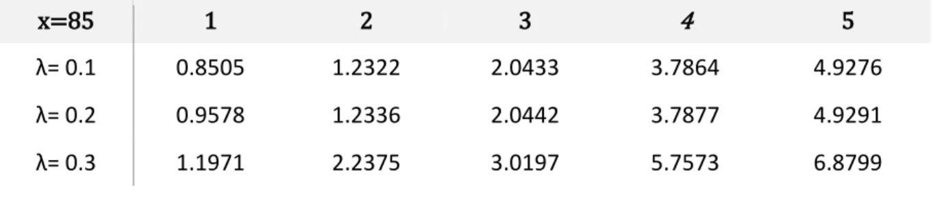
x=85 1 2 3 4 5

λ= 0.1 0.8505 1.2322 2.0433 3.7864 4.9276 λ= 0.2 0.9578 1.2336 2.0442 3.7877 4.9291 λ= 0.3 1.1971 2.2375 3.0197 5.7573 6.8799

3.2. TEST II – SWAP PRICING USING SURVIVAL PROBABILITIES THROUGH THE

SIMULATEDMEAN:MALE

After testing female data, we calculated the longevity swap premiums based on male data, for both countries. The results in basis points are presented for US (table 4) and Japan (table 5), where we depict the premiums values for the different maturity, ages and longevity risk premium levels, as was done for female data.

Analysing the premiums value from tables 4 and 5 it is possible to verify that, as observed in female data, the maturity has a positive effect in the swap premium since, for all ages, the premium value is higher for longer maturities. Beside this effect, the age at contract initiation still has a key role in this framework, since as expected when the age increases the swap premium value increases too. The higher swap premium is registered for 5 year contracts based on 85 year old individuals at contract initiation in both countries. This relationship between age and maturity is accompanied by the longevity risk premium effect. The risk, as exposed in female results, has an increase effect in premium values, across all ages and maturities. As in female results, these tendencies follow an expectancy survival framework and are observable in both countries, including a micro analysis, due the fact of US male data register higher premiums than Japan male date.

Table 4- Swap Premiums for different maturities and risk using US Male data (2010-2014)

x=65 1 2 3 4 5 𝜆 = 0.1 0.0827 0.1444 0.8977 1.5900 2.6498 𝜆 = 0.2 0.0864 0.1494 0.9060 1.6014 2.6659 𝜆 = 0.3 0.0904 0.1540 0.9137 1.6119 2.6807 x=75 1 2 3 4 5 λ= 0.1 0.1886 0.5523 0.9710 1.6901 2.7909 λ= 0.2 0.1884 0.5537 0.9707 1.6897 2.7903 𝜆 = 0.3 0.1882 0.5557 0.9703 1.6891 2.7895

30

x=85 1 2 3 4 5

λ= 0.1 1.2399 2.2177 3.0193 4.7560 4.9159 λ= 0.2 1.2820 2.2226 3.0273 4.7670 5.8991 λ= 0.3 1.3207 2.2279 3.0361 4.7789 6.8836

Table 5 - Swap Premiums for different maturities and risk using Japan Male data (2010-2014)

x=65 1 2 3 4 5 𝜆 = 0.1 0.0878 0.1329 0.8821 1.5683 2.6205 𝜆 = 0.2 0.0924 0.1428 0.8966 1.5907 2.6519 𝜆 = 0.3 0.0990 0.1493 0.9072 1.6029 2.6675 x=75 1 2 3 4 5 λ= 0.1 0.1897 0.5211 0.9731 1.6930 2.7943 λ= 0.2 0.1907 0.5343 0.9746 1.6949 2.7967 𝜆 = 0.3 0.1926 0.5414 0.9775 1.6987 2.8036 x=85 1 2 3 4 5 λ= 0.1 1.1314 2.2281 3.0346 4.0805 5.9083 λ= 0.2 1.1619 2.2368 3.0510 4.2774 5.9359 λ= 0.3 1.2353 2.2422 3.0599 4.7976 6.9458

3.3. SENSITIVITYANALYSIS:AGES,RISKANDGENDERS

The results presented above showed a few macro tendencies, however its feasible comparing female and male data directly and verify the advantages and disadvantages of both results. In this section we conduct a sensitivity analysis to the results provided above by considering and comparing female and male scenarios for ages 65 and 85 and two types of risk level.

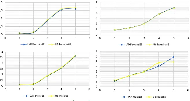
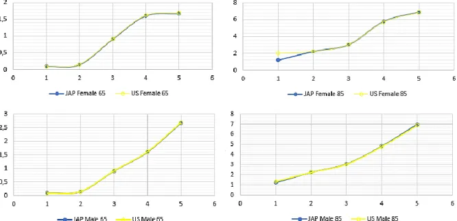
In figure 9 we exhibit the results for male and female data for 65 and 85 years, using 0.1 as our longevity risk premium. The first observable conclusion is that for 65 years the female premiums are between 0 and 2 and for the male premiums they range between 0-3, so a slight difference exists. This tendency is still observed when we use the 85-year old reference cohort. Due to this, is possible to verify that, independent of the age used as reference, the effect of the risk premium level in swap prices is the same.

31

However, male data is significantly different from female data since, as the figure 9 shows, the female values are smoothed, and the main tendency still the same for the two ages and maturities. In other ways, male data shows a different effect. The effect in male premiums for 85 years old is different than 65 old years, since for 65 years we’ve a smoothed behavior and, nonetheless, for 85 years the US male data registers a higher value for all maturities, excluding for 5-year contracts for which Japan contracts are more expensive than US equivalent contracts. Beside this effect, when comparing directly male data with female it is possible to notice that the swap premium values for the 65-year old female cohort tends to stabilize between maturities 4 and 6, while male premiums continue to increase in a proportional way. For 85 years old the behavior is different, since for females we’re having a proportional increase in both countries, and for males while US data suffers a stabilization Japan data still increase proportionally.

Figure 9 – Female and Male premiums for 65 and 85 ages and risk level 0.1

After testing and reporting the comparison between male and female data for a risk level of 0.1, was tested the same data for a risk level 0.3. The results are reported in figure 10. In this figure it is possible to verify that the risk level affects all results (for male, female 65 and 85 years old contracts) in the same way, since all premiums value increase significantly. Due to this, as confirmed above, the level of risk affects all data in the same way.

Comparing with the previous scenario both data (US and Japan) register a smooth behavior. Analyzing 65-year old contracts results it is possible to verify that female data increase with the maturity, however, there is an inclination to stabilize between maturities 4 and 5, while male data increase in a direct way for all maturities. For higher reference ages the premiums

32

performance is also identical for both genders and countries: an increase. While for lower risk level the performance was slightly different.

Please note that for all scenarios US data has the higher premiums when comparing directly with Japan, and independently of the sex considered (excluding for 85 years old with λ= 0.1) .

33

5. CONCLUSION

In our days, longevity is a reality in developed and developing countries. Insurers and reinsurers around the world find themselves in a fragile condition to cover this risk efficiently and profitably. Considering this need, this paper aims to demonstrate how derivatives, typical of financial markets, can be used to manage longevity, overcoming the problem of calculating their premium and fair value.

Taking this goal into account, it was possible to calculate some longevity swap premiums, for different scenarios, by forecasting the force of mortality, (assuming the dynamics of mortality) and by using log bilinear Lee-Carter model under a Poisson setting, and estimated survival probabilities using US and Japan, after transforming this adding the risk through the Wang transform and risk-neutral simulated technique. With this technique we could simulate different longevity swap premiums for 65, 75 and 85 years old and for both genders using US and Japan data. Across this analysis, it was noticeable that the risk level and maturity have a positive effect in premium values, increase them independent of the age or gender used. Was notorious that premium values for male data are higher than female, independent of the years old used as reference. For different years old we obtained a different result, higher for higher ages and lower for lower ages. These tendencies follow an expectancy survival framework, and are observable in both countries, since when the age increase the survival probability will be lower and the amount requested to cover that event would be higher. The same is applied for the risk level and maturity, since when the risk and maturity is higher the investor should have a better return and the swap is more valuable.

The market for longevity remains a poorly exploited market for its absorption by financial markets, and this article makes a significant contribution to the aid calculating its premiums and fair values. For further investigation, it is recommended to apply this approach to more derivative instruments, for example options, and using different type of input data, such as survival or mortality index. Given the simplicity of this methodology, it enables a series of comparative analyses that should be explored in future studies, filling the gaps of research on longevity.

34

4. REFERENCES

Alho. J.M. (2002). Discussion of Lee (2000). North American Actuarial Journal 4 (1). 91- -93.

Barrieu. P.. Bensusan. H.. Ravanelli. C. e Hillairet. C. (2012). Understanding. modeling and managing longevity risk: key issues and main challenges. Scandinavian Actuarial Journal 2012:3. 203-231. Barrieu. Pauline and Veraart. Luitgard A.M. (2014) Pricing q-forward contracts: an evaluation of estimation window and pricing method under different mortality models. Scandinavian Actuarial Journal . ISSN 0346-1238 (In Press) DOI: 10.1080/03461238.2014.916228

Batini. N.. Callen. T.. & McKibbin W.(2006). The global impact of demographic change. Working paper. International Monetary Fund.

Bauer. D.. Börger. M.. & Ruß. J. (2010). On the pricing of longevity-linked securities. Insurance Mathematics and Economics. 46. 139–149. http://doi.org/10.1016/j.insmatheco.2009.06.005

Bensusan. H.. El Karoui. N.. Loisel. S.. & Salhi. Y. (2016). Partial splitting of longevity and financial risks: The longevity nominal choosing swaptions. Insurance Mathematics and Economics. 68. 61–72. http://doi.org/10.1016/j.insmatheco.2016.02.001

Blake. D.. & Burrows. W. (2001). Survival Bonds: Helping to Hedge Mortality Risk. Journal of Risk & Insurance. 68(2). 339.

Blake. D.. Cairns. A.. Coughlan. G.. Dowd. K.. & MacMinn. R. (2013). The New Life Market. Journal of Risk & Insurance. 80(3). 501–558. http://doi.org/10.1111/j.1539-6975.2012.01514.x

Blake. D.. Cairns. A.. Dowd. K. (2006). Living with mortality: longevity bonds and other mortality-linked securities. British Actuarial Journal. 12 (1). 153–228.

Blaschke. E. (1923). Sulle tavole di mortalità variabili col tempo. Giornale di Matematica Finanziaria 5. 1-31.

Bravo. J. Freitas. N. (2017). Valuation of longevity-linked life annuities. Insurance Mathematics and Economics. DOI: https://doi.org/10.1016/j.insmatheco.2017.09.009

Brorsen, B. & Fofana, N. (2001). Success and failure of agricultural futures contracts. Journal

of Agribusiness, 19, 129-145.

Brouhns. N.. Denuit. M. e Vermunt. J.K. (2002). A Poisson log-bilinear regression approach to the construction of projected lifetables. Insurance: Mathematics and Economics 31. 373-393

Cairns. A. J. G.. Blake. D. e Dowd. K. (2006). A two-factor model for stochastic mortality with parameter uncertainty. The Journal of Risk and Insurance 73 (4). 687-718.

Carlton, D.W. (1984). Futures markets: Their purpose, their history, their growth, their successes and failures. Journal of Futures Markets. 4, 237-271.