The impact of exhaustibility on commodity prices

Master Degree in Finance from the NOVA – School of Business and

Economics.

The impact of exhaustibility on commodity prices:

An event study approach

Matteo Timpano

29973

A Project carried out on the Master in Finance Program, under the

supervision of:

Martijn Boons

Abstract

The objective of this work is to study the impact of exhaustibility on spot and futures prices of a specific set of resources, whose future limited availability and low substitutability performance have been highlighted by scientific papers. I modelled exhaustibility as a set of events, which might raise investors’ awareness regarding the intrinsic scarce nature of the commodities selected. I conducted an event study using ordinary least squares regressions for nine commodities over the sample 10/09/1993 – 10/09/2018 with event dummy variables grouped into eight categories. Regression results assert the presence of abnormal return in correspondence with the selected occurrences; however, it is difficult to determine a universally valid pattern in terms of significance and direction of the effect.

Keywords: exhaustibility, commodities, event study. JEL Classification: Q31; G14; G23.                                   Note: this brief note is meant to inform the jury that the present version of the work project was written starting from a longer one (65 pages) delivered for Maastricht University as part of the Double Degree program on December 17, 2018.  

1. Introduction

Institutional investors worldwide have been paying careful attention to investment opportunities in commodities market. Investing in commodities essentially means investing in raw materials that might be used for direct consumption or for the production of by-products. Financial innovation has produced a vast set of tools through which investors today might gain exposure towards the price fluctuations of raw materials. Irwin and Sanders (2011) outlined how the “financialization” of commodity markets played an important role in this sense. Thanks to the abundance of financial instruments, the volume of investment in commodity markets has grown significantly. Research conducted in 2008 by the Commodity Futures Trading Commission (CFTC) revealed that the total notional value on June 30, 2008 of all futures and options open contracts for the 33 U.S. exchange-traded markets was $945 billion.

However, examining the performance of commodities, we often tend to think that they will be indefinitely available in the future. There are commodities that are widely traded on a daily basis whose future availability is still uncertain. Base metals, oil, land and water are just a few of the commodities that are present only in limited quantities on our planet. The issue of scarcity of resources has created a harsh debate among economists and it dates back to the seventeenth century. Thomas Malthus (1798) was the first economist to clearly include in his work the concept resource scarcity, connecting it with population growth and poverty. Building upon this principle, future research in natural resource economics led to the famous Hotelling’s rule (1931), formulated by Harold Hotelling, who described the price path of an exhaustible natural resource: in a perfectly competitive market, with no extraction costs, the price of a natural resource must rise at the market rate of interest. The work of Sundaresan (1984) represents a further evolution of his work. In a competitive market structure, the spot price is expected to increase at a rate exceeding the risk-free rate in the interval of time between discoveries and that the extent to

which this rate exceeds the risk-free alternative depends on the specific nature of the commodity examined. My initial intuitive guess regarding exhaustibility was that a commodity with decreasing level of reserves would increase in price as its remaining stocks are progressively depleted. Scarce and exhaustible resources would then represent a suitable opportunity for those institutional investors that have a long run investment horizon, which might match the remaining life of the commodity in question. Therefore, I decided to conduct my research as a background analysis of commodities’ markets to determine how prices react in the presence of events that might possibly make the market aware of the limited availability of a certain set of resources. This work is an interdisciplinary research that stems from the strong theoretical knowledge developed by scholars of natural resource economics on scarce commodities and it aims at bringing its main intuitions to a more practical level in the context of financial markets. The existing financial literature in fact typically focuses on analysing the impact of macroeconomic announcements on commodity prices.

The research question that I will try to answer with this work is therefore: “what is the impact of exhaustibility on commodity prices?” or more specifically, “what is the impact of events affecting exhaustibility on commodity prices?” Following a step-by-step procedure, I will develop an empirical analysis to verify whether commodity market prices react to a selected amount of events, which might question the future availability of the material.

The first step of this procedure is to formulate a clear definition of exhaustible resource. Secondly, I should determine a set of suitable commodities to be analysed as exhaustible with a careful analysis of scientific papers, which would help me to determine what are the materials’ characteristics to be taken into account and to scientifically validate the analysis. Thirdly, I need to review the literature on commodities, extending the notions presented in the previous paragraph to better understand how studies on commodity prices are usually conducted and what

main conclusions have been drawn. Fourthly, I should outline how event studies with commodities prices are performed and the paper of McKenzie, Thomsen, and Dixon (2004) is particularly useful in this sense as they assess the inferential accuracy of several event study methodologies using daily data on futures returns. This procedure will eventually provide an initial general understanding of how markets perceive exhaustibility. I humbly believe that my work could be seen as an extension of the literature on exhaustible resources. In the ever-changing environment we are living nowadays, investors are forced to approach and analyse investment opportunities taking into account several additional factors. It is my personal belief that evaluating the impact of environmental issues on commodity prices might be advantageous for designing new innovative investment solutions.

The main findings of the regression analysis show that there exists mixed evidence of abnormal return in correspondence of event dates. However, it is impossible to define a universally valid pattern for all commodities in the sample, since we notice differences in the magnitude and direction of the effects. Panel data analysis helps in creating a general perspective on the direction of the effects, but the presence of mixed evidence in the outcomes urges a commodity-specific interpretation of the impact, which pooled OLS tends to neglect. A simple qualitative study of historical volatility of commodity futures prices reveals that some of the significant events selected occurred in in intervals of time leading up to volatility peaks, which would confirm the need to account for exhaustibility among the factors producing price uncertainty. The rest of the paper is organized as follows. Chapter 2 presents the research conducted to review the literature on the various fields needed to implement the empirical analysis. Chapter 3 outlines the event study methodology, the data used and the commodity and event selection processes adopted. Chapter 4 introduces the main results obtained and Chapter 5 discusses them. Finally, Chapter 6 includes the major implications of the results and final considerations.

2. Literature Review Exhaustible Resources

Studying natural resources is not an obvious matter. Humanity has been dealing with resource scarcity since the dawn of history and it has continuously challenged generations of our species to find innovative solutions to survive. Studying this issue from a financial perspective cannot disregard its inherent interdisciplinary nature and the need to connect sources and ideas coming from completely different fields. This is the reason why the path followed for this work embraces three main literatures: theoretical natural resource economics, science (geology and ecology) and empirical finance. Kneese (1988) also acknowledged this particular perspective, depicting how the study of natural resource economics has forced scholars to reach out beyond the traditional boundaries of their disciplines and to integrate knowledge coming from a plethora of fields such as physics, chemistry, ecology, biology and more.

The starting point of my thesis is to define clearly what an exhaustible or non-renewable commodity is, relying on the natural resource economics literature. Kneese (1988) defined depletable or non-renewable resource as those materials such as minerals and energy commodities for which only a limited stock exists for its allocation over all time. Following Kneese (1988) research, Malthusian theories can be seen as the first approach to natural resource economics. Malthus (1798) theorized that the misalignment between the rate of growth of population and resources would condemn the majority of the population to survive in low living standards. Cameron and Neal (2002) criticized the so-called “law of diminishing returns”: they claimed that the productivity-enhancing technological and institutional innovations have postponed the realization of Malthus’ prophecy. History confirmed that the extreme assertion made by Malthus in 1798 was not true, but resource scarcity still creates issues in underdeveloped nations. As more developing countries emerge, their population will increase and

the rate at which they will deplete resources will rise. This uncertainty makes interesting to review how academics have studied resource scarcity throughout the years.

One of the basic results in non-renewable resources literature is the theory of Harold Hotelling (1931), who formulated the famous Hotelling’s rule. The basic Hotelling model outlined the implications of the finite availability of a non-renewable resource on its price and its optimal rate of extraction. In Hotelling’s frictionless world, the return to holding the non-renewable resource asset is exactly the increase of its in situ value. This value will increase at the market rate of interest for the effect of market equilibrium. Concisely, Krautkraemer (1998) explained that Hotelling’s rule can be summarized with this statement “in the case of zero marginal extraction costs, the price of the resource equals the in situ value and so the resource price would also increase at the rate of interest” (pp. 2066). However, Krautkraemer (1998) explained that some implications of Hotelling’s work failed to be consistent when more complex reality aspects were included in the initial model. Subsequent works in the field of natural resource economics have tried to overcome the excessive simplicity of his model by incorporating more complex elements in their theories. In particular, many scholars focused on the analysis of market structures to determine how the price trajectory of an exhaustible resource would evolve under market conditions such as competition and monopoly. Weinstein and Zeckhauser (1975) focused their research towards the allocation of scarce resources: they claimed that a competitive market structure was able to produce the socially optimal allocation of exhaustible resources and an exponentially increasing price trajectory of the resource at the marginal rate of time preference in society. Conversely, the presence of a monopolist would generally cause over conservation of the resources since they would limit supply to suboptimal levels for society. Stiglitz (1976) compared the rate of exploitation of an exhaustible resource under competitive and monopolistic regimes assuming constant elasticity of demand together with zero extraction costs. The main result

presented by Stiglitz is that in both regimes, we would obtain the same spot price trajectory of the resource. Increasing the complexity of the framework, he relaxes the assumption of constant elasticity of demand substituting it with increasing elasticity. This results in a higher rate of increase in the price in the competitive market with respect to the monopoly. This outcome is consistent with the conclusion of Weinstein and Zeckhauser (1975), as the monopolist tends to over conserve the resource using a slower “rate of utilization” (pp. 657).

Levhari and Pindyck (1981) developed a theoretical model constructed as a more comprehensive extension of Hotelling’s including resource durability, as a durable resource provides utility even when it is stored and not used and its demand is for “quantities of stock in circulation, rather than for flows of production and depend on expected changes in price as well as the current price level” (pp. 366). They conclude that the general price path for an exhaustible and durable resource is typically U-shaped. One of the cases is particularly interesting for this paper: in the presence of partial durability of the exhaustible resource and growing demand, it is possible to obtain an extreme case where we have a continuously rising path for the price.

Sundaresan (1984) conducted a more comprehensive study developing an equilibrium valuation model of natural resources with the objective of studying the intertemporal optimal extraction policy to derive the equilibrium spot price behaviour of the exhaustible resource under competition and monopoly. Differently from the literature reviewed so far, the author included elements of potential uncertainty within the model. Sundaresan (1984) argues that the spot prices under the monopolistic structure are generally higher than in the competitive setting, since the monopolist implements a more conservative policy and the reserve level is usually higher. The price evolution predicted by the author is increasing in periods between discoveries and discontinuous drops occur in correspondence of successful discoveries. However, spot prices between discoveries rise at a higher rate in a competitive regime with respect to a monopoly. To

sum up, in presence of uncertainty elements and in a competitive market setting, the spot price is expected to rise at a rate greater than the risk free rate and the extent to which such rate exceeds the risk-free alternative depends on the nature of the specific exhaustible resource examined. The factors that cause this difference are price elasticity of demand, the mean arrival rate of discoveries and the magnitude of new available reserves.

To have a final broad view regarding exhaustible resources, we can complement the results obtained by Sundaresan (1984) with the study of Krautkraemer (1998). The definition of exhaustible resource seems to be generally accepted by scholars as a material with finite availability for allocation over time. This distinctive character of these resources brought academics to study the potential evolution of their price trajectories. The initial model formulated by Hotelling (1931) has frequently failed to explain the “dynamic behaviour of non renewable resource prices and in situ values” (pp. 2102). Krautkraemer (1998) highlights how models able to incorporate exploration, capital investment and heterogeneous ore quality factors performed better at describing the price paths. However, the variety of other additional factors influencing price dynamics made impossible for the literature to clearly define models that are able to connect the theoretical knowledge with observed empirical results. On the one hand, Krautkraemer (1998) also reports that empirical evidence has shown that technological progress and the discovery of new reserves have mitigated the impact of exhaustibility of commodities: the research of new substitutes for certain materials and the technical improvement of processes are likely to continue to mitigate scarcity. On the other hand, though, he also acknowledges that future scenarios are still uncertain and “whether or not these mitigating factors will keep pace with increased demand for non-renewable resources (…) remains to be seen” (pp. 2103).

What seems to be certain is that the presence of scarcity creates uncertainty: there could be an upward potential for prices of exhaustible resources endowed with combined finite availability and limited substitutability.  

Critical Commodities: Supply Risk and Low Substitute Performance

In 2011, the European Commission (EC) created the list of critical raw materials (CRMs), a document that analyses a set of critical commodities, which are both fundamental for the European economy and associated with a high risk of supply. In the last criticality assessment, European Commission (2017) has examined 78 non-energy and non-agricultural materials. In order to identify a critical material, the study on the review of the list of Critical Raw Materials takes into account two criteria: first, the economic importance (EI) of the material or the “importance of a given material in the EU end-use applications and performance of its substitutes in these applications” and secondly, the supply risk (SR) that measures “the risk of disruption in supply of a given material”. The results of the criticality assessment indicate the existence of twenty-six critical materials (see Appendix A). European Commission (2017) states that the issue with these materials is to ensure a stable supply coping with their increasing demand. Fast moving technological innovations and the growth of emerging markets represent a tough challenge for an import-dependent economy such as the one of European Union (EU). Many of the commodities included in the CRM list also have the negative characteristic of being geographically concentrated in certain areas of the world and this increases the probability of supply disruption. European Commission (2017) reports that this probability is further enhanced by the fact that many stages of the extraction and production process of these materials occur in a small number of countries. Despite being the CRMs document a reliable institutional source to start from, it is necessary to conciliate the scientific sources examined with the availability of

data: most of the materials included in the list are not frequently traded on financial markets and there are not many financial instruments that use them as underlying asset. Therefore, I decided to review also papers that examine the exhaustible nature of more common commodities.

Killick (2008) defined base metals as the “quintessential exhaustible resource” since the mineral deposits from which we extract base metals are not renewable and they cannot be synthesized in any way. Graedel, Harper, Nassar and Reck (2015) propose a careful analysis on the potential substitutability of materials for their major applications with the objective of assessing to what extent modern society is dependent on the availability of materials. Historically, the presence of scarcity for materials has spurred researchers to develop new extraction methods or new suitable substitutes. Graedel et al. (2015a) conducted their research trying to evaluate the best-performing substitute for all metals and metalloids of the periodic table in their major uses. Several widely used materials such as copper, lead, chromium and manganese have no immediate substitute for the major uses. Moreover, none of the elements subject of their analysis has a substitute that ensures a suitable performance for its main applications. The absence of substitutes in case of severe shortage would lead to worsening of product performance and increase in price. Graedel, Harper, Nassar, Nuss and Reck (2015) also studied the criticality of metals, but they enlarge their research using a more complex and comprehensive methodology to assess criticality of 62 elements of the periodic table. In a graph where the y-axis is vulnerability to supply restrictions and x-axis is the supply risk, Graedel et al. (2015b) distinguish two clusters of metals with interesting values. The first notable cluster (Cluster 5 in the original graph) is composed of lead, tin, rhodium and tellurium, which have midrange values on both axes. The second cluster (Cluster 4) contains those metals with relatively high values on the x-axis: antimony, selenium and indium are all materials widely used in technological applications. It seems that metals that

constitute a concern in terms of supply risk are important for high-tech applications since these metals are scarce and normally extracted as by-products.

Elshkaki, Graedel, Ciacci and Reck (2018) proposed a different perspective since they focused their attention on seven major metals. This paper approaches the issue of metal criticality constructing a scenario-based study to assess empirically what could be the future evolutions of demand-supply imbalances for these fundamental materials. The “major metals” group includes seven known metals, which are iron (Fe), aluminium (Al), manganese (Mn), copper (Cu), zinc (Zn), lead (Pb), and nickel (Ni). Calculating the expected cumulative demand for each metal, they estimate that the nickel, iron, manganese and aluminium do not show any immediate concern of significant demand-supply imbalance. Copper, lead and zinc demand instead is expected to cross the level of global resource production by 2050.

There are four key takeaways provided by this brief overview. Firstly, the perfect example of a non-renewable resource with limited substitutability seems to be metals. Secondly, scholars generally study criticality assessing it using current availability of the material and performance of its substitutes. Thirdly, many studies reached the conclusion that there exists a set of commodities for which a special attention is needed in order to preserve their future stable supply because technological progress is affecting the demand for these commodities. Finally, other researchers have shown how a group of more common metals also need special attention since a demand scenario reveals potential future imbalances in the demand-supply relationship.

Commodity Spot and Futures Prices

The next logical step of this analysis is to review the most common and reliable approaches with which the fluctuations of commodity prices are typically analysed. There exists a major branch of the literature regarding commodities that is devoted to the study of commodity-linked

investments’ returns. The most popular instrument analysed by scholars are definitely commodity futures. Gorton and Rouwenhorst (2006) defined futures markets are defined as “forward looking” (pp. 48) since the determination of the fair futures prices comes from the expectations of economic agents about the future spot price that will prevail in the future. The return that comes from acquiring a future position is the risk premium or the difference between the current futures price and the expected futures spot price. Following the work of Gorton, Hayashi and Rouwenhorst (2012), it is possible to divide the commodity futures literature in two main strands. The first one is the theory of storage introduced by Kaldor (1939), which describes the convenience yield as the implicit benefit of holding the commodity inventories and it is a negative function of the inventory level. Keynes (1930) instead developed the second fundamental theory called normal backwardation, which assumes that the commodity producers or inventory holders hedge their exposure towards commodity price fluctuations by taking a short futures position and in order to convince speculators to buy the contract, they sell it at a discount. Other papers have focused on describing the performance and the main characteristics of commodity futures as single investment or as portfolio element. The attractiveness of commodity-linked investments derives primarily from three key characteristics: satisfactory return performance, diversification benefits and inflation-hedging power. Gorton and Rouwenhorst (2006) constructed an equally weighted index of commodity futures and they found out that their index provided a comparable performance in terms of return with a substantially lower downside risk. Moreover, their correlation analysis result highlighted how commodity futures might also constitute a better inflation hedge than stocks and bonds. Some studies revealed that the inclusion of commodity futures within investors’ portfolios could deliver enhanced portfolio returns. The study of Jensen, Johnson and Mercer (2000) has proved that in a risk/return optimization, substantial weight was assigned to commodity futures over a sample

data of 25 years and they assume an even more prominent role in optimal allocation during restrictive policy periods. The diversification argument is also supported by many other studies that have a more critical perspective regarding the allure of commodity futures as investment. Sanders and Irwin (2012) claimed that the positive portfolio performance found in previous works stems mainly from diversification, which is not a guarantee of positive returns. A similar claim is contained in the work of Erb and Harvey (2006), who recognized the potential value of commodity futures as a portfolio component: if a portfolio of commodity futures reaches an adequate level of diversification, historical data show that it might deliver positive returns. The other property commonly associated with commodity futures is inflation hedging. The empirical findings regarding this property are mixed. Gorton and Rouwenhorst (2006) have described that commodity futures have higher sensitivity to unexpected inflation and in the opposite direction of stocks and bonds. Erb and Harvey (2006) and Ang (2014) also examined the sensitivity of individual commodity futures and they agree that the inflation sensitivity depends on the type of commodity. Edwards and Park (1996) consider instead show that with managed futures investments, there is evidence of a positive and significant correlation between yearly percentage changes in Consumer Price Index (CPI) and annual rates of return of futures.

The remaining part of this section presents a more specific part of the commodity markets literature, which mostly concerns with the sensitivity of commodity spot and futures prices to events or macroeconomic announcements. There exist both theoretical and empirical studies examining the responses of spot and futures prices to the unanticipated changes of a variety of macro variables. The theoretical model of Bond (1984) focused on the impact of permanent and transitory supply and interest rate shocks on commodity prices. Subsequent research has developed empirical studies about commodity prices. The paper of Barnhart (1989) analysed the impact of the unanticipated component of thirteen macroeconomic announcements on commodity

spot to determine what macroeconomic disturbances have an effect on commodity markets. In general, commodity prices are mostly influenced by money supply, Federal Reserve discount rate, manufacturers’ orders of durable goods and housing starts. The sign of these responses is negative in most of the cases proving the validity of the policy anticipation hypothesis. Other papers have investigated the efficacy of monetary policy using its impact on commodity prices. Frankel and Hardouvelis (1985) and Frankel (2008) exploited the flexible nature of raw materials ‘prices to show that expansionary monetary intervention are often associated with a negative commodity price response as agents anticipate a monetary tightening.

Within the financial literature studying commodity prices sensitivity, academics widely investigated the fluctuations of two shiny metals, gold and silver, which historically had the role of store of value. Christie-David, Chaudhry and Koch (2000) and Cai, Cheung and Wong (2001) both studied how news releases affect the prices of these two commodities. Both these works found that gold futures respond strongly to unemployment, GDP, and CPI announcements, consistently with the research of Frankel and Hardouvelis (1985). Christie et al. (2000) showed that silver instead reacted significantly to news on unemployment rate and capacity utilization. Elder, Miao and Ramchander (2012) extended the high frequency data analysis of their colleagues using a larger time span and verifying the impact of announcements on three variables returns, volatility and trading volume. Their analysis includes both gold and silver prices together with a base metal, copper. Early morning news releases have a strong impact on volatility of all three commodities but as for returns, only silver and copper returns react significantly. Being gold and silver usually considered as store of value, their returns react negatively to unexpected and positive news releases about economic activity. The opposite behaviour is instead observable in copper returns, reflecting its importance as industrial metal.

Roache and Rossi (2009) compared the behaviour of gold not only with copper, but also to the one of other commodities in correspondence of scheduled and periodic macroeconomic announcements using Generalized Auto Regressive Conditional Heteroscedasticity (GARCH) specification. Their empirical evidence suggests that gold exhibits counter cyclicality, mainly caused by the fact that agents tend to anticipate future monetary tightening when a positive inflation surprise occurs. In turn, this generates high real interest rates and lower gold prices. (see Frankel and Hardouvelis, 1985 and Barnhart, 1989). The results also corroborate the classical store of value and safe-heaven role of gold during bad times. Conversely, the other commodities, including agricultural products and base metals, are positively affected by higher-than-expected economic activity, as in Elder et al. (2012).

Caporale, F. Spagnolo and N. Spagnolo (2017) developed a vector autoregression-generalized autoregressive conditional heteroscedasticity approach to model the dynamic linkages of both mean and variance of macro news and commodity returns. The mean spillovers are positive for all the commodities considered except for gold and silver, which conserve their counter cyclical nature also found in other works. As for the other commodities, negative news has a significant impact on aluminium, corn and wheat but neither positive nor negative news seem to have an impact on copper, platinum and soybeans. As for volatility, positive and negative news have a significant impact on the volatility of many commodities independently from the positive or negative nature of the event. This is true for all commodities except for gold, whose volatility spillovers coming from negative news are substantially larger.

Overall, the evidence coming from this branch of the literature shows that individual commodity prices exhibit some degree of sensitivity to the occurrence of certain macroeconomic events. However, the extent to which this response is significant depends on the commodity itself.

3. Research Design

The aim of this chapter is to present in detail the methodology chosen for this thesis.

I used daily spot or futures price data for nine selected commodities, which are Silver, Copper, Lead, Zinc, Tin, Water, Cocoa, Antimony and Tungsten. The commodity selection process has been conducted relying on notions coming from scientific papers and reports such as the CRM list. The majority of these materials are not widely known and it was difficult to find commodity-linked instruments to determine the impact of events on this set of materials. The next logical step was to consult different sources of information coming from scientific literature. Crossing the information coming from papers and institutional sources, it is easy to notice that different works often end up considering roughly the same set of commodities, even if different evaluation mechanisms clearly produce small differences. However, many materials highlighted as most critical by these scientific sources were clearly less popular compared to widely known commodities. It is necessary to find a trade off between work originality and the need for identifying a set of commodities which the reader could be familiar with. Elshkaki et al. (2018), Graedel et al. (2015b) and Graedel et al. (2015a) were extremely useful since they also examined the future potential criticality of widely known metals. Combining the results of these papers, the group of major metals analysed is composed of silver, copper, lead, tin and zinc. After having selected this group of traditional metals, I decided to include in the group two less popular materials. These are a semi metal, antimony, and a rare metal, tungsten. Antimony and tungsten are both included in the critical raw material list of the European Commission since its earliest version. Secondly, they are particularly vulnerable as they are both subject to high geographical concentration and China is their major supplier, which holds respectively 87% and 84% of global supplies of these two materials, according to the EC document. Thirdly, antimony has a technical connection with other materials because it is often used in an alloy together with other metals.

In the attempt of increasing the originality of my work, I also decided to include two extra commodities as part of the research. These are water and cocoa. Water is a vital commodity for the life on our planet and it has absolutely no immediate substitute. FAO (2007) reports that 1.2 billion people live in areas where physical scarcity is part of their daily reality. The water crisis that hit the city of Cape Town last year is one of the most frightening episodes of our recent history. Being extremely essential, water can only be studied in the context of financial markets with ETF, constructed as a bundle of stocks of companies that operate in the water management and distribution sector. The application of an event study on water ETFs has the obvious disadvantage that the returns considered would be equity returns. Cocoa is the only agricultural commodity included and its harvests are constantly in danger because of climate change. European Commission (2015) in the factsheet on agriculture and climate change states that most of the changes to climatic conditions will have a negative impact on crops. For this reason, the list of commodities selected includes cocoa. Scott (2016) explained how rising temperatures and lack of humidity have been impacting cocoa crops in Ivory Coast and Ghana.

Data and Time Interval

The dataset used consists daily price data for the nine commodities selected using both spot and futures prices over the period 10/09/1993 – 10/09/2018. Unfortunately, using some unusual commodities creates obstacles in terms of availability of data. This required adapting data to the type of commodity. The futures prices series are settlement price continuous series coming from London Metal Exchange (LME) for copper, tin, lead and zinc; continuous series for silver is retrieved from the Chicago Mercantile Exchange and cocoa futures price is taken from International Exchange (ICE). A detailed description of spot and futures price series can be found in the Appendix B. As for antimony and tungsten, futures prices are not available; therefore spot

prices are used to construct the returns. Unfortunately, it is not easy to verify the impact of events on these commodities for two main reasons. First, there are not futures instruments that use them as underlying. Second, the small amount of trading that involves these instruments causes the price trajectory of antimony and tungsten to have a constant price for relatively long intervals in the sample selected. To overcome this limitation, the study of these two commodities requires using spot prices with both daily and weekly frequency over the period 15/10/1993 – 09/10/2018. Finally, water scarcity is addressed performing the event study on daily returns of four water ETFs over the period. These are Invesco Global Water, Invesco S&P Global Water, iShares Global Water and S&P Global Water. The time interval chosen for this commodity is 14/06/2007 – 09/10/2018. This sample is shorter than the others simply because it corresponds to a time frame during which all the instruments selected are contemporaneously quoted.

The choice of performing regressions with both spot and futures prices enriches the analysis with an additional source of comparison. From traditional finance theory, we know that futures markets are forward looking. Under the efficient market hypothesis (EMH), spot prices should be the result of all the publicly available information. The use of spot and futures prices might help us compare the immediate effect of exhaustibility with its impact on future expectations.

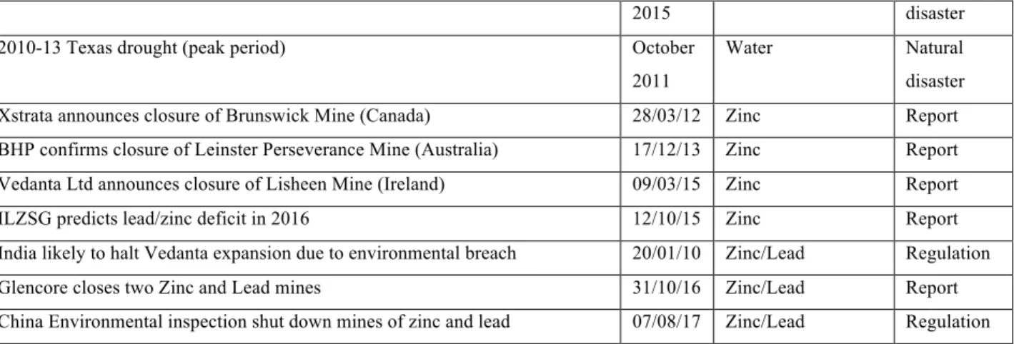
As far as the choice of events is concerned, I conducted a careful selection of events following two main criteria: first, I prioritized those events that happened in countries extensively involved in the supply chain of the commodity. Secondly, I chose events that might produce a signal of future scarce supply of the commodity. In Appendix C, a detailed description of the procedure and the complete list of the events are provided.

Estimation Strategy: Ordinary Least Squares (OLS)

The main reference for the empirical section is the work of McKenzie et al. (2004), in which they evaluated the accuracy of different event study approaches in terms of size and power of test. Among the different methodologies studied, I decided to apply the ordinary least squares (OLS) regression with event dummies to perform my analysis. The OLS approach described in McKenzie et al. (2004) estimates the abnormal return as coefficient of dummy variables, which correspond to event dates. This regression tests that the average abnormal return on event date is statistically different from zero; therefore, if the event has some influence on the dependent variable commodity price, the event dummy should be significant. On the one hand, the main flaw of this model is that commodity futures returns often show heteroscedasticity, which might violate the assumptions of the OLS estimation, leading to biased estimates. McKenzie et al. (2004) reveal that a GARCH specification does not lead to superior performance in terms of size of tests compared to a simpler OLS estimation strategy. The estimation strategy is a standard regression method that can be written as:

𝑅!= 𝜃!𝑥!+ 𝛽𝐸!+ 𝜀! (1)

The dependent variable 𝑅_! is the daily return on the commodity spot or futures prices. The return is calculated as the logarithmic return, meaning that 𝑅_!= ln 𝑃_!!! 𝑃_! . The vector 𝑥_! usually contains a constant term and a series of non-event related explanatory variables. McKenzie et al. (2004) report that past studies have used a variety of series to control for different effects. In this work, the only explanatory variable is a broad world equity index, MSCI World Index, which represents the performance of large and mid-cap stocks coming from 23 developed economies. The dummy variable 𝐸! takes value of one on event dates and zero otherwise. In this work, the event window is (-3; +3) days around the event date, meaning that the dummy variables are equal to one for a total of seven observations. The dummy variables are used to capture the effect of the

event and 𝛽, the coefficient of the dummy, is interpreted as the average abnormal return on event dates. The dummies inserted in the various regressions performed are grouped into event categories. This particular structure allowed me to verify the impact of not only single events, but also event groups, which is more meaningful for this analysis. All the events are grouped into eight categories. These are: “NATURAL DISASTER”, “REGULATION”, “TRADE”, “REPORT”, “STRIKE”, “WAR”, “MARKET” and “WATER CRISIS” (only for water).

4. Empirical results

The aim of this chapter is to present the empirical results of my analysis. The first section presents the descriptive statistics of the data used. The second section introduces the main results obtained by the OLS regressions. Thirdly, the results of a basic pooled OLS regression provide a further source of comparison.

Descriptive Statistics

The interpretation of some descriptive measures helps us to have a much clearer idea of the data being used to perform the subsequent regressions. The descriptive statistics of the nine commodities are presented in Tables 1 – 4. All commodities considered have a similar daily average return and this return is not extremely different from zero. Over a sample of 6522 observations, tungsten is the commodity whose spot price exhibits the highest average daily return of 0.036%. The lowest average return is instead measured for cocoa and it amounts to 0.010%. The median has a value of zero for all the commodities and it is a more robust measure for the centre of the distribution. In terms of standard deviation, the commodities considered have similar values since for all of them it ranges between 1% and 2%. Antimony and tungsten are the materials with the lowest values. Conversely, silver, zinc, lead and cocoa are the ones that

reach the highest values of standard deviation. Both the S&P index and MSCI index have lower daily volatility over the same period. The return distribution is clearly non-normal for the entire set of commodities: they all exhibit negatively skewed distributions, high level of kurtosis, which signals high frequency of extreme outcomes, and the probability associated with the Jarque Bera (JB) test assumes a value of zero for each of them. Table 4 contains the descriptive statistics for futures returns of six commodities and it is easy to notice that the values are similar to the ones of the spot price returns. An interesting difference is detectable in the skewness of futures distributions of copper and silver, which show a higher degree of skewness with respect to the values of spot prices. The same is true also for cocoa, whose futures skewedness is now slightly negative (-0.05). The distributions of futures remain leptokurtic for all commodities in the sample. This slight difference has no impact on the final evaluation on the nature of the distribution, since Jarque Bera tests confirm their non-normality.

Table 3 describes the performance of the four water ETFs analysed for this thesis. Their return performance is lower than the one of spot and futures prices of most commodities as the average daily return delivered by water ETFs is 0.0137%. However, the daily standard deviation of these instruments is inferior as its average across the four ETFs amounts to only 1.35%. Three of these water-linked instruments have a negatively skewed distribution, only the iShares Global ETF has a moderately positive return distribution (+0.33). The high kurtosis values highlight that the distribution of each of these instruments is strongly fat tailed.

Regression Results

The results are presented by commodity starting from the five major metals, then for water and cocoa and finally, antimony and tungsten. The regression framework allows us to test whether on the event dates selected, the price of the commodity produces a statistically significant abnormal

positive or negative return. Therefore, the coefficient, the sign and p-value of the dummy variables are the figures we should pay careful attention to. Each commodity price has been regressed against all dummy variables together and against each single dummy category.

Copper spot and futures price returns have been regressed against six different dummies: strike,

war, report, regulation, natural disaster and market. Table 5 presents the results of spot price regressions. In each regression, the market return is highly significant and with a large positive coefficient value. Most of the dummy variables considered are non-significant both in the general regression and at individual level. The market dummy is the only significant variable: this means that on event dates selected, the spot price of copper produces an abnormal return which is statistically different from zero. It is interesting to notice that differently from my initial intuition, we find both positive and negative coefficients for the dummy variables considered. The initial expectation was to find only positive abnormal reactions to events. The results suggest a different interpretation for copper since war, regulation and market dummies have negative coefficients. This is also confirmed by results of futures regressions: the sign and significance of the dummies’ coefficients is exactly the same as the ones examined above for spot price returns. For this reason, I also performed some extra regressions over smaller samples for some specific events. Among the different events, the war dummy, in fact, seems to be significant around the burst of the second Congo war: columns (2) – (5) of Table 7 contain regressions performed over samples of +/- three months, six months, one year and two years around the event date. The only result obtained is that the war dummy is again significant at 10% level around an interval of one year.

Silver price returns have been regressed on a regulation and market dummy variables in Table 8

and 9. Consistently with what we found for copper, the results across spot price variables do not differ too much. The market return is highly significant in both tables but its magnitude is larger for futures returns. The regulation dummy has a negative coefficient but it is not statistically

different from zero in any of the specifications. Conversely, the market dummy has a positive and significant coefficient at 10% level both in the general regression and in the individual regression. This significance is not corroborated by the results of futures returns in which the market dummy is no more significant. I decided to run some extra regressions to verify the significance of the market dummy on the futures returns series: as reported in Table 10, the event dummy is significant for five smaller samples around the event date of Berkshire Hathaway Inc. (1998) disclosure of an investment in silver due to potential demand-supply disruptions.

Table 11 and 12 present the results for tin regressions. Tin returns series are regressed against three dummy categories: war, regulation and natural disaster. Once again, market return is significant in all columns and the R-squared is approximately equal for all regressions and always close to 7%. Differently from the previous case, war and natural disaster are both highly significant for both spot and futures prices: the war dummy should have a positive impact on price, whereas natural disaster dummy has instead a negative effect. The regulation dummy has a negative coefficient as well, but it seems to be non significant for both spot and futures prices. However, since its p-value is close to 10% significance, I decided to perform some extra regressions, which are collected in Table 13, trying to verify the presence of a single significant event. It turned out that the introduction of the “Governing regulation on the realization of mineral and coal mining business activities” in Indonesia in 2010 produced a significant and negative impact on both spot and futures prices.

The fourth metal of this group is lead. Lead prices series are regressed against commodity categories of report, regulation and market. Just like for tin, we find that results are consistent across the two dependent variables considered. The market return is highly significant in all specifications with a positive coefficient. Tables 14 -15 show that the regulation and market dummies are not statistically different from zero in both general and individual regressions. The

only significant impact seems to be obtained by the report dummy, which has a positive and significant coefficient at 10% level. In addition, the value of the coefficient is equivalent in both spot and futures prices regressions (0.0042). Unfortunately, no significant result emerges examining smaller samples for both market and regulation dummies. However, Table 16 shows improved significance for the report dummy using a series of smaller samples between 2010 and 2018 for futures (2010 – 2018, 2011 – 2018, 2014 – 2018, 2015 – 2018 and 2016 – 2018).

The last metal of this group is zinc, whose returns have been regressed on five different dummy variables, meaning report, regulation, natural disaster and market. We find consistency in the estimates of market return coefficient and R-squared with respect to the previous commodities analysed: the market return is still significant and the coefficient of determination is around 8%. Table 17 shows that the spot price of zinc follows lead in terms of dummy variable significance: regulation, natural disasters and market dummy are non significant over the entire sample. The only significant dummy is report, which is positive and statistically different from zero at 1% level in both general and individual regressions. Futures regressions further confirm the results of spot price returns. Smaller samples regressions of zinc highlighted that the announcement of the closure of zinc and lead mines by Chinese environmental authority (regulation) has a significant impact on spot and futures zinc prices, as reported in Table 19.

Cocoa is the only agricultural commodity involved in this analysis. The spot and futures returns

of cocoa have been regressed against a total of five dummy variables: war, report, trade, natural disaster and market. The results reported in table 20 and 21 are a bit disappointing with respect to the expected outcome. Unfortunately, none of the dummy variables is significant over the entire sample considered and the R squared of each regression is lower than 1%. Extra regressions reported in Table 22 reveal that only the publication of the Cocoa deforestation report by Higonnet, Bellantonio and Hurowitz (2017) for the environmental organization Mighty Earth

(report) is significant for spot and futures prices. Measuring exhaustibility on water is particularly challenging. Water cannot be traded as futures. Therefore, an alternative solution is to examine the impact of a set of events on exchange traded funds. Table 23 presents the regressions for the four ETFs including all dummy variables considered, which are natural disaster, report, war and water crisis. Unfortunately, none of those produces significant results. It is also not possible to define a pattern for the significance of the dummy variables across the four instruments. Water ETF and S&P Global Water ETF and both negative in the case of Invesco S&P Global Water ETF. As for iShares Global Water ETF instead, only the report dummy has a positive coefficient. This last regression is also the one that achieves the lowest R squared value (0.22), substantially lower than the other regressions whose coefficient of determination is always higher than 0.60. The reasons for these outcomes will be discussed later in Chapter 5.

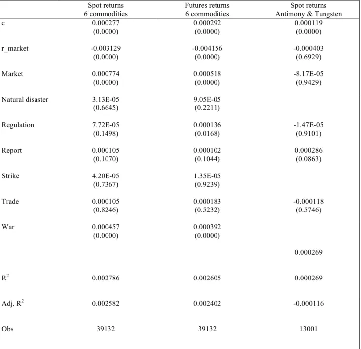
The last two commodities included in this work are antimony and tungsten. The results for the complete regressions are reported in Table 24. The first result to highlight is the negative relationship of antimony and tungsten spot price returns with the market return: at weekly frequency, the market return coefficient is negative and significant at 5% level for antimony and at 10% level for tungsten. This significance is not observable in daily data, though. At a weekly frequency, there are no significant dummy coefficients for both commodities. However, some interesting results are observable in daily data: the regulation dummy, for example, is negative and significant at 10% for antimony, whereas the report dummy is positive and significant for tungsten at 1%. In order to improve my analysis, I also examined smaller samples for both commodities. The initial significance of the regulation dummy is confirmed by the extra regressions for antimony in Table 25 and 26: in all four subintervals, regulation dummy is significant at 1% level in daily data. It is interesting to notice the different magnitude of the coefficients in the two data frequencies: the regulation dummy coefficient is larger for weekly

rather than daily data. Table 27 reports the additional analysis on the report dummy for tungsten, which is again positive and significant at 10% for both subsamples of weekly data.

Pooled Regressions

Pooled regressions basically consists in pooling together in one single vector the returns of every commodity, disregarding their commodity-specific nature, and regressing them against the market return and the vectors of the each dummy variable category using ordinary least squares. In other words, the model specification is as follows:

𝑅_!,! = 𝛽_!𝑟_!"#,!+ 𝛽_!𝐸_!,!,!+ ⋯ + 𝛽_!𝐸_!,!,!+ 𝜀_!,! (2)

The vector 𝑅_!,! contains the returns for a group of commodities and it is regressed against 𝑟_!"#,!, meaning the return on the market, and a group of event categories variables. Tables 28 – 30 present the result of this exercise. The results of a general regression including all dummy variable categories and six commodities using futures returns show that: firstly, the market return is significant at 1% with a large coefficient (0.46). Secondly, dummy variables market and natural disaster have a negative sign, whereas dummy variables regulation, report, strike, trade and war have a positive sign. Thirdly, the only significant dummies are market (5%), report (1%) and trade (5%). The first column of Table 28 illustrates the outcomes of a general regression using spot price returns. The market return is significant at 1% with a large coefficient (0.42) as in the previous case. While the dummy variables market, natural disaster and regulation have a negative sign, the other event categories of report, strike, trade and war have a positive coefficient value. Once again, we only have two significant dummies, market (5%) and report (1%). Pooled regression of Table 30 (column 1) includes only two commodities since tungsten and antimony were observed on a different sample with respect to the other materials. It shows that the market return is non-significant, trade and regulation dummies have a negative sign,

whereas report and market have a positive sign. Report is the only significant event dummy for antimony and tungsten and it is statistically different from zero at 1% level.

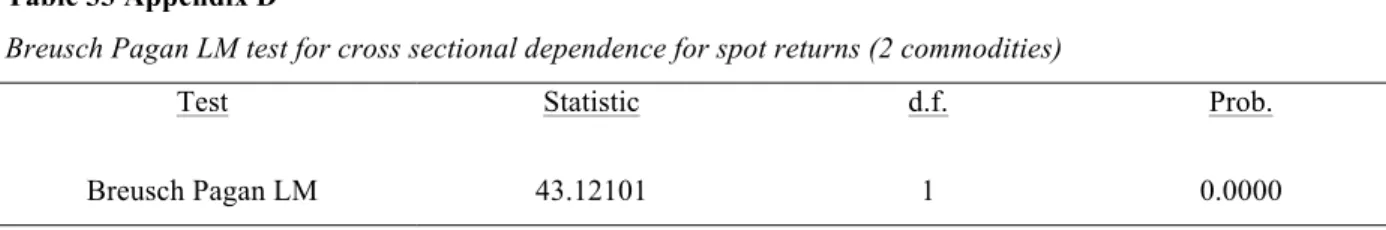
This pooled OLS analysis is useful as an extra insight regarding the signs of the coefficients, but it disregards the individual specific effects of each commodity. In particular, a test on residual cross sectional dependence has highlighted the presence of correlation in the residuals in all three regressions (see Appendix D). Since this would risk to severely impair the results of this part of my analysis, I tried to apply a Cross Section Seemingly Unrelated Regression (SUR) on my panel data to address this cross sectional dependence. The results of this possible solution are reported in Table 29 and in the second column of Table 30 for antimony and tungsten. The pooled OLS with cross section SUR of the first six commodities for spot price returns highlights that the market dummy is significant at 5% level and negatively related to the price, whereas the report dummy is still positive, but no more significant. Two other dummy variables are now significant: trade and war dummies are both significant at 10% with a positive coefficient. As for futures returns, the sign and significance of the market and war dummy are true also for futures, but trade dummy seems not to be significant anymore. The cross section SUR correction for antimony and tungsten is reported in the second column of Table 30 and it provides additional confirmation of the previous result: the report dummy has a positive coefficient and it is still highly significant at 1% level.

5. Discussion

This chapter contains a subjective analysis of the results presented in Chapter 4. The regressions performed have two main purposes: first, to determine whether commodity prices react significantly to the occurrence of the selected events, producing abnormal return. Secondly, they should shed some light regarding what type of event category has the biggest effect on each commodity and thirdly, they should give some indications regarding the magnitude of the

reaction and whether this is different across commodities and price variables. In addition, performing regressions on smaller subsamples aims at verifying the impact of single events. The descriptive statistics section has allowed us to determine that these commodities are generally a riskier stand-alone investment with respect to a general equity index. Having examined each commodity individually, it is necessary to highlight that this was an expected and perfectly normal result. All commodities exhibit a level of standard deviation higher than the one of the equity indices and negatively skewed distribution of returns. In addition, fat-tailedness of their spot and futures returns further confirms this, as high values of excess kurtosis are typically associated with the more frequent occurrence of extreme events.

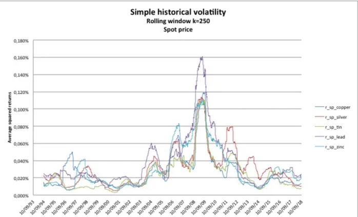
A more precise outline of the risk profile of each commodity can be obtained by extending the previous brief observations regarding the historical volatility estimates. Modelling historical volatility of these commodities is not the purpose of this work, but it is useful to compare the risk profile of the materials. Figure 1 – 5 show the results for each commodity spot and futures prices. It is interesting to notice how the five major metals approximately move together and they experienced a low volatility environment until 2003, except for cocoa that had one big spike between 2003 and 2004, which other commodities experienced only partially. Volatility levels increased inevitably during the crisis for all commodities and they started going back to the same level of the nineties with the only exception being silver, which experienced two additional spikes. Historical volatility estimates for antimony and tungsten (Figure 4) reveal that the tungsten estimate is consistently higher than the one of antimony, whose highest volatility values are registered at the beginning and at the end of the sample. Figure 5 shows the historical volatility estimates for the water ETFs. We can immediately detect that for the entirety of the sample the four instruments move together. Their volatility is particularly high during the crisis period but for the rest of the sample, their volatility is never higher than 0.034%. In my opinion, a

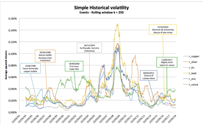
particularly instructive exercise is to connect the amount of information included in this volatility estimates with the focus of my work, meaning the response of commodity prices to events. In Figure 6, I included seven events in the graph of futures simple historical volatility. The temporal positioning of these occurrences is interesting. For instance, consider the event occurred on June 13, 1996 and its impact on copper futures prices volatility. The action of the famous speculator Yasuo Hamanaka is situated right before a mild spike in copper volatility. The same is true for all the other examples: Warren Buffet disclosure of his large investment in silver happened in correspondence of a peak in the silver series and the burst of the first Ivory Coast war occurred before a substantial spike in cocoa futures volatility. The Sumatra Earthquake (tin), the announcement of the closure of Lisheen Mine (zinc) or the announcement of closure for two Glencore plc mines (lead) are other clear examples. The presence of empirically significant exhaustible-related events in intervals of time leading up to historical volatility peaks might suggest that among infinite array of factors that affect commodity price volatility, the exhaustible nature of certain commodities plays a role that should not be neglected. A further confirmation of this observation is provided in Appendix E.

After this brief digression regarding volatility, it is time to lay out the key outcomes suggested by the regression analysis proposed in the previous chapter. In my opinion, these results reveal the following fundamental aspects: first, there is evidence of abnormal return, either positive or negative, on the event dates selected. Differently from my initial intuition, several commodities show a negative reaction to certain categories of events. This outcome urges the need for a thorough explanation that inevitably involves both potential model misspecifications and particular aspects of the single commodity market, which are apparently not captured by the model. This brings us to the second main result of the analysis: it is not possible to define a pattern of dummy significance common to the entire set (or small subsets) of the commodities.

While it is possible to claim that exhaustibility might play a role in volatility estimates, it is still unclear whether a potential future disruption creates a positive-only spike in the price of all commodities. Each commodity reacts differently to the types of event categories in question; hence this calls once again to try to consider the nature of the commodity itself to determine why one type of event is significant for a commodity and completely irrelevant for the others. The third general takeaway retrieved from the results concerns the magnitude of the effects produced by the significant dummy variables. As explained previously, we interpret the coefficient of the dummy variable as the abnormal return associated with the occurrence of the event. Therefore, there is a further aspect worth mentioning. The magnitude of the response is approximately equal across the two price dependent variables (with a couple of notable exceptions) and it presents some substantial differences when considering the impact of distinct event categories.

First of all, let us consider the discrepancy between the expected effect on commodity price and actual realized sign of the dummy variable coefficient, which in many cases assumes a negative value. A general explanation of this phenomenon could be given by formulating a reasoning that is similar to the concept of the “policy anticipation hypothesis”. This theory is definitely far from the main subject of this thesis but the intuition behind it might be useful to partially explain why we see these negative coefficients in front of some of the dummy variables. As outlined by Barnhart (1989), under the policy anticipation hypothesis, market agents perceive an unexpected increase in money supply as a money demand shock, which will be counteracted in the future by the central bank, since it is committed to follow its initial mandate. Therefore, they expect that in the future the central bank would counteract this measure with a monetary tightening and this expectation translates in the present with an immediate rise in the level of real interest rates. The same logic can be applied to our case on commodities. In Chapter 3, the work of Graedel et al. (2015b) pointed out that historically, society has been able to counteract to shortages of critical

materials with technological improvement that developed suitable solutions. Despite the fact that there is no evidence that this kind of behaviour is going to persist in the future, it might be possible that these episodes constitute reliable proof of the ability of society to counteract to critical materials’ shortages. Investors might be aware of this historical trend and they expect that this behaviour will be consistently repeated in the future. A similar belief would trigger an expectation mechanism that brings investors to expect a rate of growth of technology and a future decrease in price that is instead effectively realized in the present.

Pooled regressions might be a useful instrument to understand the economic logic behind exhaustible events and commodity prices. Panel data analysis reveals that the only dummy variable with a negative and significant coefficient is the market dummy. In both specifications (with and without the cross section SUR correction), market events seem to produce a negative effect on commodity price. The other significant variables have a positive coefficient. This mixed evidence convinced me to focus more carefully on individual commodity regression with respect to panel data. The reason for this is that the single commodity market dynamics are probably affecting the efficacy of the model: there might be some specific characteristics that the current specification is not able to capture. Notwithstanding this, if we compare the results over the entire sample of observations, most of the dummy variables, when significant, have a sign consistent with the results of the panel data analysis. This pattern might mean that panel data regressions are not completely misleading as for the direction of the impact on commodity prices, but they do not furnish satisfactory results for the significance of dummy variables.

The expectation mechanism might be a plausible explanation for the negativity of certain coefficients, but it cannot be applied universally to the entire set of commodities. Its universal validity would imply that the existence of a unique market condition common to every commodity in the sample, which is clearly not realistic. Despite the fact that scientific papers

have highlighted their criticality, it does not necessarily mean that the same degree of limited substitutability and future availability can be assigned to each commodity. Therefore, the effect that exhaustibility has on commodity prices is proven, but the direction of such effect can only be explained with a careful commodity specific research. Within the limits of this research, it is now my intention to draw the attention of the reader to the effect of exhaustible events on single commodities. A clear example of the concept outlined above is the significance of the market dummy on copper and silver prices. As for copper, the market dummy is negatively significant, whereas for silver it takes a positive coefficient value. In the case of silver, the coefficient positivity can be easily justified, as the event causing this positive relationship is Warren Buffet’s disclosure of a big silver investment due to potential supply disruptions in the silver market: a well known and recognised investor like Buffet is able to increase the awareness of other market agents towards a potential rise in price caused by silver shortage. The negativity of copper is more complicated to explain. The significance of the event dummy is probably given by the implementation of the speculative strategy of the trader Yasuo Hamanaka, who controlled 5% of world copper production in 1995. This episode has been included in the exhaustibility related set because it reveals how the concentration of copper production in the hands of one single individual might cause potential supply disruptions. However, it was impossible to assign a specific date to verify the impact of this strategy, therefore I opted for June 13, 1996, which is the day in which Hamanaka reported losses for his positions. The choice of this event might prove that the end of this cornering attempt relieved investors from their fears of a high degree of concentration in copper production. In my opinion, this is the cause of the negative coefficient in front of the market dummy for copper prices. The negative coefficient in front of the war dummy is a different case. Smaller samples regressions revealed that the burst of the second Congo War was significant in a one-year interval around the event date. The beginning of a military conflict