André Cordeiro Valério
The Impact of Uncertainty and Commodity
Prices on Emerging Economies
André Cordeiro Valério
The Impact of Uncertainty and Commodity Prices on
Emerging Economies
Dissertação apresentada ao Centro de De-senvolvimento e Planejamento Regional da Universidade Federal de Minas Gerais, como requisito parcial à obtenção do título de Mes-tre em Economia.
Universidade Federal de Minas Gerais – UFMG
Centro de Desenvolvimento e Planejamento Regional – CEDEPLAR
Programa de Pós-Graduação em Economia
Supervisor: Mauro Sayar Ferreira
Ficha Catalográfica
V164i 2016
Valério, André Cordeiro.
The impact of uncertainty and commodity prices on emerging economies [manuscrito] /André Cordeiro Valério. – 2016.
96 f.: il., gráfs.
Orientador: Mauro Sayar Ferreira.
Dissertação (mestrado) - Universidade Federal de Minas Gerais, Centro de Desenvolvimento e Planejamento Regional.
Inclui bibliografia (f. 54-56).
1. Mercado futuro – América Latina - Teses. 2. Bolsa de mercadorias – América Latina – Teses. 3. América Latina - Política econômica - Teses. 4. Incerteza - Teses. I. Ferreira, Mauro Sayar, 1972- . II. Universidade Federal de Minas Gerais. Centro de Desenvolvimento e Planejamento Regional. III. Título.
André Cordeiro Valério
The Impact of Uncertainty and Commodity Prices on
Emerging Economies
Dissertação apresentada ao Centro de De-senvolvimento e Planejamento Regional da Universidade Federal de Minas Gerais, como requisito parcial à obtenção do título de Mes-tre em Economia.
Trabalho aprovado. Belo Horizonte, 26 de fevereiro de 2016:
Mauro Sayar Ferreira
Orientador
Gilberto de Assis Libânio
CEDEPLAR/UFMG
Sérgio Luís Guerra Xavier
IBMEC-MG/FIEMG
“Scientific knowledge is a body of statements of varying degrees of certainty – some most unsure, some nearly sure, none
absolutely certain.”
Resumo
Esse trabalho estuda o impacto de choques de incerteza e de preços de commodities em
cinco economias latino-americanas exportadoras líquidas de commodities: Brasil, Chile,
Colômbia, México e Peru. As análises foram feitas através de Vetores Autoregressivos Estruturais Bayesianos (BSVAR) com restrições na estrutura recursiva. Um choque que reduz a incerteza da economia global eleva o preço decommodities. A reação das economias
é quase similar à de um choque positivo em preço decommodities: redução no risco soberano,
apreciação cambial, aumento do PIB. Contudo, o impacto inflacionário não necessariamente será o mesmo em ambos os choques. Choque puro nos preços dascommoditiesgera inflação,
apesar da apreciação cambial. Mas elevação no preço das commodities devido a reduções
na incerteza sobre a economia global não gera impacto inflacionário relevante por causa do canal financeiro: há maior apreciação cambial devido à intensa queda no prêmio de risco soberano. Banqueiros centrais devem interpretar de forma adequada a origem das oscilações nos preços de commodities para que possam conduzir política monetária de
forma consistente.
Palavras-chave: Choques internacionais; Incerteza; Preço de commodity; Política
Abstract
This work analyzes how five Latin American economies (Brazil, Chile, Colombia, Mexico and Peru) are impacted by shocks in the world economy uncertainty and in commodity price. Analysis is based on Bayesian Structural Vector Autoregressions (BSVAR) with block exogeneity. A shock that reduces global uncertainty increases commodity price. The economies react almost as similar as in the case of a pure (positive) shock to commodity price: sovereign risk falls, exchange rate appreciates, and GDP increases. However, the inflationary impact is not necessarily the same. A pure commodity price shock generates inflation, despite the nominal exchange rate appreciation. But an increase in commodity price due to reduction in global uncertainty is not as inflationary because of the financial channel: the nominal exchange rate appreciation is more profound due to a more intense contraction in sovereign risk. Central bankers need to properly interpret the origin of oscillations in commodity price to conduct monetary policy appropriately.
Keywords: External shocks; Uncertainty; Commodity prices; Monetary policy; Emerging
List of Figures
Figure 1 – Monthly U.S. stock market volatility. Source: Bloom (2009) . . . 29
Figure 2 – The importance of commodities for Brazil, Chile, Colombia, Mexico and Peru . . . 41
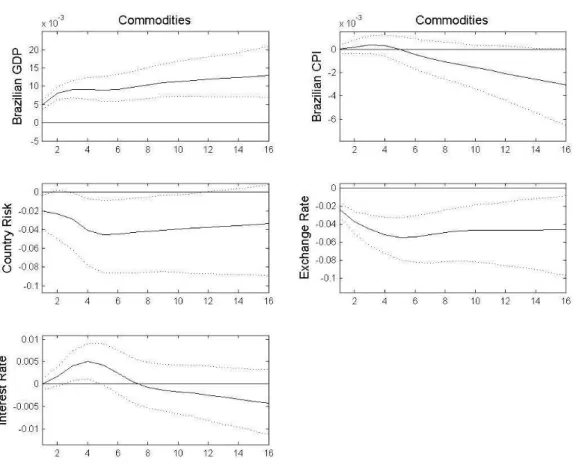
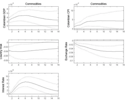
Figure 3 – Response of Brazilian variables to a commodity price shock . . . 42
Figure 4 – Response of Brazilian variables to a VIX shock . . . 44
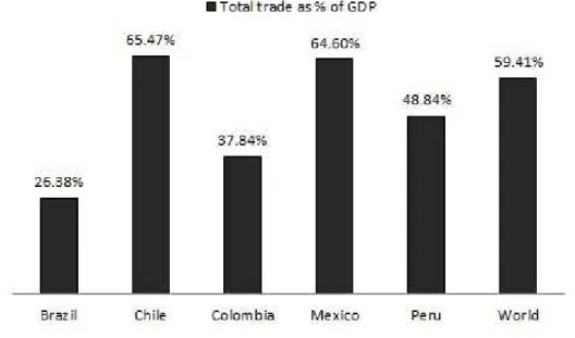
Figure 5 – Economic openness of Brazil, Chile, Colombia, Mexico and Peru with 2013 data. . . 46
Figure 6 – Response of Brazilian variables to a commodity price shock . . . 48
Figure 7 – Response of Brazilian variables to a VIX shock . . . 49
Figure 8 – Response of international variables . . . 58
Figure 9 – Response of Chilean variables to a commodity price shock . . . 59
Figure 10 – Response of Chilean variables to a VIX shock . . . 59
Figure 11 – Response of international variables . . . 60
Figure 12 – Response of Colombian variables to a commodity price shock . . . 60
Figure 13 – Response of Colombian variables to a VIX shock . . . 61
Figure 14 – Response of international variables . . . 61
Figure 15 – Response of Mexican variables to a commodity price shock . . . 62
Figure 16 – Response of Mexican variables to a VIX shock . . . 62
Figure 17 – Response of international variables . . . 63
Figure 18 – Response of Peruvian variables to a commodity price shock . . . 63
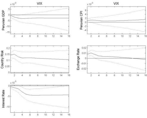
Figure 19 – Response of Peruvian variables to a VIX shock . . . 64
Figure 20 – Response of international variables . . . 64
Figure 21 – Response of international variables . . . 66
Figure 22 – Response of Chilean variables to a commodity price shock . . . 67
Figure 23 – Response of Chilean variables to a VIX shock . . . 67
Figure 24 – Response of international variables . . . 68
Figure 25 – Response of Colombian variables to a commodity price shock . . . 68
Figure 26 – Response of Colombian variables to a VIX shock . . . 69
Figure 27 – Response of international variables . . . 69
Figure 28 – Response of Mexican variables to a commodity price shock . . . 70
Figure 29 – Response of Mexican variables to a VIX shock . . . 70
Figure 30 – Response of international variables . . . 71
Figure 31 – Response of Peruvian variables to a commodity price shock . . . 71
Figure 32 – Response of Peruvian variables to a VIX shock . . . 72
Figure 33 – Response of international variables . . . 72
Figure 35 – Response of Brazilian variables to a VIX shock . . . 74
Figure 36 – Response of international variables . . . 74
Figure 37 – Response of Chilean variables to a commodity price shock . . . 75
Figure 38 – Response of Chilean variables to a VIX shock . . . 75
Figure 39 – Response of international variables . . . 76
Figure 40 – Response of Colombian variables to a commodity price shock . . . 76
Figure 41 – Response of Colombian variables to a VIX shock . . . 77
Figure 42 – Response of international variables . . . 77
Figure 43 – Response of Mexican variables to a commodity price shock . . . 78
Figure 44 – Response of Mexican variables to a VIX shock . . . 78
Figure 45 – Response of international variables . . . 79
Figure 46 – Response of Peruvian variables to a commodity price shock . . . 79
Figure 47 – Response of Peruvian variables to a VIX shock . . . 80
Figure 48 – Response of international variables . . . 80
Figure 49 – Response of Brazilian variables to a commodity price shock . . . 81
Figure 50 – Response of Brazilian variables to a VIX shock . . . 81
Figure 51 – Response of international variables . . . 82
Figure 52 – Response of Chilean variables to a commodity price shock . . . 82
Figure 53 – Response of Chilean variables to a VIX shock . . . 83
Figure 54 – Response of international variables . . . 83
Figure 55 – Response of Colombian variables to a commodity price shock . . . 84
Figure 56 – Response of Colombian variables to a VIX shock . . . 84
Figure 57 – Response of international variables . . . 85
Figure 58 – Response of Mexican variables to a commodity price shock . . . 85
Figure 59 – Response of Mexican variables to a VIX shock . . . 86
Figure 60 – Response of international variables . . . 86
Figure 61 – Response of Peruvian variables to a commodity price shock . . . 87
Figure 62 – Response of Peruvian variables to a VIX shock . . . 87
Figure 63 – Response of international variables . . . 88
Figure 64 – Response of Brazilian variables to a commodity price shock . . . 88
Figure 65 – Response of Brazilian variables to a VIX shock . . . 89
Figure 66 – Response of international variables . . . 89
Figure 67 – Response of Chilean variables to a commodity price shock . . . 90
Figure 68 – Response of Chilean variables to a VIX shock . . . 90
Figure 69 – Response of international variables . . . 91
Figure 70 – Response of Colombian variables to a commodity price shock . . . 91
Figure 71 – Response of Colombian variables to a VIX shock . . . 92
Figure 72 – Response of international variables . . . 92
Figure 74 – Response of Mexican variables to a VIX shock . . . 93
Figure 75 – Response of international variables . . . 94
Figure 76 – Response of Peruvian variables to a commodity price shock . . . 94
Figure 77 – Response of Peruvian variables to a VIX shock . . . 95
List of Tables
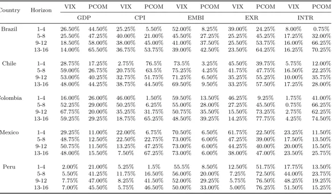
Table 1 – Standard deviation of growth rates of emerging economies . . . 16 Table 2 – Standard deviation of growth rates of developed economies . . . 16 Table 3 – Standard deviation of consumption growth rate of emerging economies . 17 Table 4 – Standard deviation of consumption growth rate of developed economies 17 Table 5 – Forecast error variance decomposition of international shocks - Baseline
model . . . 65 Table 6 – Forecast error variance decomposition of international shocks - Extended
Contents
Introduction . . . . 14
1 WHAT WE KNOW ABOUT EMERGING ECONOMIES AND THEIR CYCLICAL FLUCTUATIONS . . . . 16
2 EMPIRICAL MODEL . . . . 28
2.1 The dataset . . . 28
2.2 Methodology . . . 30
2.3 Priors . . . 33
2.4 Identification . . . 38
3 THE ROLE OF UNCERTAINTY AND COMMODITY PRICES SHOCKS IN EMERGING ECONOMIES . . . . 41
3.1 Commodity price shock . . . 41
3.2 Uncertainty shock . . . 43
3.3 The relative importance of uncertainty and commodity prices shocks . . . 45
3.4 Trade balance channel and foreign exchange interventions . . . . 45
3.4.0.1 Commodity prices shock . . . 47
3.4.0.2 Uncertainty shock . . . 49
3.4.0.3 Summary . . . 50
3.4.0.4 The relative importance of external shocks in the extended model . . . 51
4 CONCLUDING REMARKS . . . . 52
BIBLIOGRAPHY . . . . 54
APPENDIX
57
APPENDIX A – IMPULSE RESPONSE FUNCTIONS - BASELINE MODEL . . . . 58A.1 Brazil. . . 58
A.2 Chile . . . 59
A.3 Colombia . . . 60
A.4 Mexico . . . 62
APPENDIX B – FORECAST ERROR VARIANCE DECOMPOSITION 65
B.1 Baseline model. . . 65
B.2 Extended model . . . 65
APPENDIX C – IMPULSE RESPONSE FUNCTIONS - EXTENDED MODEL . . . . 66
C.1 Brazil. . . 66
C.2 Chile . . . 67
C.3 Colombia . . . 68
C.4 Mexico . . . 70
C.5 Peru . . . 71
APPENDIX D – IMPULSE RESPONSE FUNCTIONS - ROBUSTNESS CHECK . . . . 73
D.1 VIX responding to commodities . . . 73
D.1.1 Brazil . . . 73
D.1.2 Chile . . . 75
D.1.3 Colombia. . . 76
D.1.4 Mexico . . . 78
D.1.5 Peru . . . 79
D.2 VIX responding to commodities and country risk not blocked. . . 81
D.2.1 Brazil . . . 81
D.2.2 Chile . . . 82
D.2.3 Colombia. . . 84
D.2.4 Mexico . . . 85
D.2.5 Peru . . . 87
D.3 VIX following an AR(4) and country risk not blocked . . . 88
D.3.1 Brazil . . . 88
D.3.2 Chile . . . 90
D.3.3 Colombia. . . 91
D.3.4 Mexico . . . 93
D.3.5 Peru . . . 94
14
Introduction
How commodity prices shocks affect emerging economies? To what extent are uncertainty shocks important to business cycle fluctuations in these economies? And most importantly, what are the challenges that these shocks impose to policymakers in emerging markets? This work tries to address these questions by providing new pieces of evidences on business cycles fluctuations in emerging economies using data from five Latin American countries: Brazil, Chile, Colombia, Mexico and Peru, all net exporters of commodities. By estimating a Bayesian Structural Vector Autoregression with block recursion, the main channels through which such shocks are transmitted can be identified and empirical regularities emerges, showing how the economic responses distinguishes from those of developed countries.
Most of Latin American countries are net exporters of commodities, and the commodity sector represent a great share of GDP, which makes these countries highly dependent on their commodity exporting sector. In the last decade (2000), Latin American economies observed an economic boom coinciding with a positive cycle in the world price of commodities. In several occasions, inflationary pressures appeared, but in others not. It is therefore important to understand in more detail how oscillations in commodity price are channeled through these economies. More specifically, when should we expect inflationary pressures and when we should not. This understanding is essential for an appropriate response of monetary policy.
After the oil crisis of the 70’s and 80’s, advanced economies observed a sharp reduction in the volatility of business cycles fluctuations, which has been referred as “The Great Moderation”. However, the financial crisis of 2007 has put an end in “The Great Moderation”, and it has been observed an increase in volatility, especially in stock markets. Higher volatility implies that economic uncertainty has risen as well and this has prompted several studies to analyze how uncertainty shocks affects the real economy. At least since Keynes (1937), which proposed that investment is the most volatile component of aggregate demand, especially because it depend of the agents’ evaluation of the future, it has been acknowledged that uncertainty has real impacts, although it did not exist good measures of uncertainty to reasonably evaluate its impacts. Bloom(2009) proposed that uncertainty would be well proxied by stock market volatility, which has also been considered by several studies.
Introduction 15
international capital leaving emerging countries, seeking safer harbors. As it will be laid out in section 1, the responses in advanced economies are not necessarily the same.
Given the main interest of the paper, which is to evaluate the impact of oscillations in commodity prices in emerging economies that are net exporter of commodities, it is extremely important to consider global uncertainty. The reason, as it will be shown, resides on the fact that commodity prices react to global uncertainty shocks. Being able to disentangle the source of this price variation becomes extreme relevant for policy makers, since the source of oscillation affects differently an economy. Although Kilian (2009) has made the argument for this distinction, considering the oil market, the literature has not yet considered both variables jointly in order to properly understand their impacts on the dynamic response of emerging economies.
The main results are that a rise in commodity prices has expansive effects throughout Latin American economies, increasing GDP and accelerating inflation. A reduction in economic uncertainty will increase commodity prices as well, however, the effects on these economies are much stronger, since this shock is also intensively transmitted through financial channels: country risk falls by a factor of 7.5 stronger when compared to a pure commodity shock, provoking similar difference in the nominal exchange rate appreciation. The impact on product and inflation will then be clearly different. It follows that monetary policy should react differently depending on the source of commodity price change.
I expand the baseline econometric model to verify if the responses would modify when controlling for interventions in the foreign exchange market. However, the variables’ responses do not alter considerably from the baseline model. Nevertheless, it is worth mentioning that intervention was detected for all economies, with magnitude varying with the nature of the shock. This suggest that these economies follow an inflation targeting regime with two targets and two instruments, as pointed by Ostry, Ghosh e Chamon
(2012).
16
1 What we know about emerging economies and their cyclical
fluc-tuations
Emerging economies are considered to be more vulnerable to economic fluctuations. In fact, there are several empirical regularities that show that real business cycles in emerging economies are substantially different from developed countries. The latter have seen a significant reduction of output volatility from the mid-80’s until the eclosion of the last financial crisis, in a period known as “The Great Moderation”. Some scholars argue that this stability was caused by better economic policies, specially those focused in controlling inflation, with the adoption of Taylor Rule and a monetary policy more predictable.
To see how volatility differs among developed and emerging economies, table1
1 shows the standard deviation of output2 per capita growth rate of selected emerging
economies from 1950 until 2009, while table 2 shows the output per capita growth of select
developed economies.
Table 1 – Standard deviation of growth rates of emerging economies
Period Argentina Brazil Chile Colombia Mexico Peru Uruguay Venezuela 1950-2009 0.052 0.037 0.049 0.021 0.034 0.05 0.054 0.054 1950-1986 0.046 0.038 0.055 0.018 0.033 0.04 0.054 0.046 1987-2009 0.062 0.029 0.031 0.025 0.033 0.064 0.054 0.067
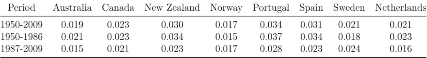
Table 2 – Standard deviation of growth rates of developed economies
Period Australia Canada New Zealand Norway Portugal Spain Sweden Netherlands 1950-2009 0.019 0.023 0.030 0.017 0.034 0.031 0.021 0.021 1950-1986 0.021 0.023 0.034 0.015 0.037 0.034 0.018 0.023 1987-2009 0.015 0.021 0.023 0.017 0.028 0.023 0.024 0.016
It is clear from tables 1 and 2 that emerging economies display higher output growth volatility. If we split the data in two periods, one from 1950 to 1986 and other from 1987 until 2009, we can see that the volatility in output growth in emerging economies has not been declining as it is observed in the set of advanced economies. The volatility has actually increased in some emerging countries after 1986.
1
The database used to construct the graphs in figures 1 to 4 was compiled by Robert J. Barro and Josef Ursua, which is available online at http://scholar.harvard.edu/barro/publications/barro-ursua-macroeconomic-data
2
Chapter 1. What we know about emerging economies and their cyclical fluctuations 17
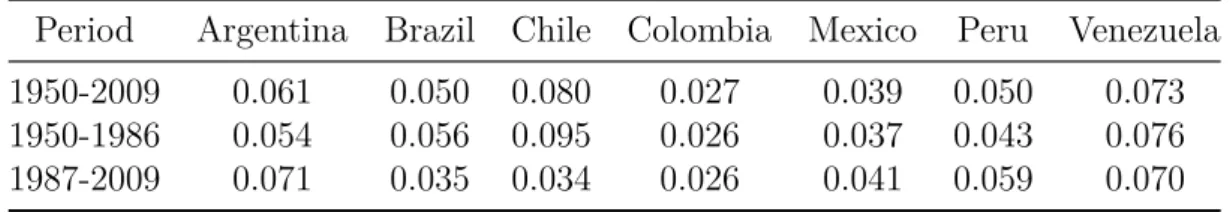
Another difference in business cycles between these two group of countries can be seen in tables 3 and 4, where the standard deviation of private consumption per capita growth rate for both sets of countries is plotted. As can be inferred by the tables,
consumption is significantly more volatile in emerging economies than in developed ones. Actually, in many of these less developed countries, the volatility of consumption is higher than the volatility of output, indicating that in emerging economies families are not able to properly use the financial system to smooth their consumption over time, suggesting a less developed financial system.
Table 3 – Standard deviation of consumption growth rate of emerging economies
Period Argentina Brazil Chile Colombia Mexico Peru Venezuela 1950-2009 0.061 0.050 0.080 0.027 0.039 0.050 0.073 1950-1986 0.054 0.056 0.095 0.026 0.037 0.043 0.076 1987-2009 0.071 0.035 0.034 0.026 0.041 0.059 0.070
Table 4 – Standard deviation of consumption growth rate of developed economies
Period Australia Canada New Zealand Norway Portugal Spain Sweden Netherlands 1950-2009 0.021 0.019 0.037 0.023 0.034 0.039 0.023 0.025 1950-1986 0.024 0.020 0.044 0.023 0.037 0.043 0.024 0.028 1987-2009 0.014 0.015 0.021 0.022 0.028 0.028 0.022 0.017
Uribe e Schmitt-Grohé (2015) treat these regularities shown in tables 1 to 4 as facts and draw some statistical evidences to support them. They show that business cycles in rich countries are about half as volatile as business cycles in emerging or poor countries. Also, not only consumption volatility is greater in emerging economies, it is more volatile than output. Finally, government consumption is countercyclical in rich countries, but acyclical in emerging and poor countries.
Therefore, these differences in business cycles fluctuations in emerging economies imposes difficulties in modelling them, since the models need to account for these singu-larities. Several studies using the Real Business Cycle (henceforth RBC) methodology have tried to explain the dynamics of emerging economies. The seminal paper of Mendoza
Chapter 1. What we know about emerging economies and their cyclical fluctuations 18
The work byCalvo, Leiderman e Reinhart(1993) find evidences that capital inflows in emerging markets are heavily influenced by external factors, in particular worldwide measures of investor‘s fear, having relevant impact in the real exchange rate and risk premium in these countries. As it will be shown, the uncertainty measure used here can be seen as investor‘s fear, therefore, their results suggests that this shock can impacted emerging economies through its effects on capital inflow.
Neumeyer e Perri (2005) extends the canonical SOE-RBC model with financial frictions to account for those empirical regularities cited above. One important aspect of their model is related to the nature of interest rate fluctuations. They assume that the interest rate faced by an emerging economy is the sum of two independent components, an international rate plus a country risk spread. Also, by assuming that firms have to pay for part of the factor of production before the production takes place, they create a channel through which the real interest rate can affect the level of economic activity. The authors model the interest rate by two means: one as a process completely independent from the fundamental shocks and other as a process that it is largely induced by these shocks. They find that the latter way can produce satisfactory results. Since the interest rate can affect the real activity through the necessity of working capital, interest rates fluctuations are induced by fundamental shocks but also amplify the effect of fundamental shocks on business cycles, contributing to high volatility. Using this model to evaluate the impact of interest rate fluctuations, they find that eliminating default risk in emerging economies can reduce about 27% of their output volatility, suggesting that country risk premium can have disturbing effects in these economies.
Chapter 1. What we know about emerging economies and their cyclical fluctuations 19
The work by Garcia-Cicco, Pancrazi e Uribe (2010) criticize studies that do not consider the particularities of emerging economies in the modelling of RBC models. Many of previous studies did not find significant differences between business cycles in advanced economies and emerging economies, therefore, in emerging economies business cycles would be driven by permanent and/or transitory exogenous shifts in total factor productivity and transmitted through the familiar mechanism of the frictionless RBC model. For instance, the studies by Kydland e Zarazaga (2002) and Aguiar e Gopinath (2007) argues that the classical RBC model can satisfactorily replicate the fluctuations observed in emerging countries data. Garcia-Cicco, Pancrazi e Uribe (2010) challenge this view, arguing that these two studies do not consider a sufficient long time series, which generate this result and that the hypothesis underlying the traditional RBC models do not well represent the reality of these economies. The authors fit a classical RBC model to Argentine and Mexican data and discover that it performs quite poorly, having not been able to explain the movements observed in the variables in the data set. Subsequently, they estimate an augmented version of the RBC model that take into account financial frictions and fit it to Argentine data and it performs really well, predicting that permanent productivity shocks explain a negligible fraction of aggregate fluctuations, giving little support to the hypothesis that the cycle is the trend.
Hevia(2014) builds a standard small open economy model for Mexico and Canada to examine the fluctuations in emerging markets. As it should be expected, he finds evidence of different responses between emerging and developed economies. By decomposing fluctuations in Mexico and Canada in terms of reduced form shocks that drive a wedge between marginal rates of substitutions and marginal rates of transformation relative to a frictionless open economy, the author finds three reduced form shocks that explain aggregate fluctuation in Mexico, which are shocks to aggregate productivity, to labor markets and to the marginal rate of substitution between leisure and consumption, while in Canada only one shock explains the fluctuation, which is a shock to efficiency and labor wedges. The author reassure the necessity of a specific modelling for emerging economies, since the classical RBC model with just productivity shocks do not provide an accurate characterization of the fluctuations in these economies.
Chapter 1. What we know about emerging economies and their cyclical fluctuations 20
trade for the small economy, increasing the prices of the imported goods relatively to the exported goods. Therefore, the net exports will be positively affected. Here, the exchange rate plays an important role in determining the pass-through to domestic inflation. The financial market channel would work as follows: supposing a rise in the interest rate of the big economy, the exchange rate of the other countries would have to depreciate. Again, the exchange rate plays an important role, because if it is fully flexible we will not observe any variation on macroeconomic aggregates. However, if this is not the case, a rise in the international interest rate will have real impacts. Additionally, the SOE-RBC literature stress that another important channel of transmission of international shocks, specially for emerging markets, are country risk premium, which are extremely dependent of international investors assessment of the current state of the world economy as well as the current state of the particular emerging economy. We would expect that a rise in country risk premium could be both because of high international uncertainty or poor performance of the local economy. As a result, the expected effects would be a shortage in external credit, occurring a “flight to quality” event, where international investors would redirect their investments to safer assets like U.S. treasury bonds.
Among the empirical works that tries to disentangle the effect of external shocks in these economies, some stand out.Cushman e Zha(1997) consider the challenges to correctly identify monetary policy under flexible exchange rates in small-open economies. Using data from Canada, they estimate a VAR that explicit imposes the assumption of small-open economy, which is done through block recursion, not allowing that international variables be affected by domestic variables. This assumption combined with the informational identifying structure used by Leeper, Sims e Zha(1996), solve all the recurrent puzzles encountered in works like this. Although they do not analyze external shocks explicitly, their methodology is very relevant to studies of small open economies, because block recursion makes the model more reasonable, assuming that the dynamics of an small open economy do not impact external variables.
The work byArora e Cerisola (2000) evaluate the impact of U.S. monetary policy over emerging economies, giving special attention to the impact on country risks. The authors find evidences that U.S. monetary policy has direct positive effects on sovereign bonds spreads. However, if investors can anticipate in some degree the effects of the American monetary policy, the impact and contagion on developing countries can be mitigated.
Chapter 1. What we know about emerging economies and their cyclical fluctuations 21
it persistently in the medium and long-run. The countries choice may be not the most interesting to assess the impact of U.S. monetary shocks, since developed and industrialized countries have more resources to deal with the possible impacts, with better institutions and better policy design. Anyhow, the author finds evidences that these shocks matter even to these countries.
Canova(2005) studies the extent and how U.S. shocks are transmitted to several Latin American countries. Using a two-step approach to identify U.S. structural shocks, he finds evidences that fluctuations in emerging economies follow a different pattern from those documented in developed economies. The main results are that U.S. real demand and supply shocks has little relative importance and small impact on these economies. On the other hand, U.S. monetary shock induces large and significant responses, through the interest rate channel. In a typical Latin American economy, a rise in U.S. interest rate is immediately followed by a rise in the domestic interest rate, which creates a large differential in favor of Latin American, resulting in capital flows, improving reserves and local aggregate demand. Therefore, U.S. monetary disturbances are turned into good output news which is exacerbated by depreciation in the real effective exchange rate which induces a temporary improvement in the trade balance. However, the trade channel seems to play a negligible role. Additionally, U.S. disturbances account for an important portion of the variability in these economies, affecting policy making because there is evidence that just putting the house in order is not enough to avoid cyclical fluctuations. Therefore, policy makers should also pay attention to developments in the American economy.
Finally, Mackowiak(2007) examine the effects of U.S. monetary policy in a set of 8 emerging economies. Using a structural VAR with block exogeneity, he finds that the interest and exchange rate reacts quickly and strongly after an American monetary shock. However, U.S. monetary policy shocks are not important for emerging markets relative to other kinds of external shocks.
More recently, a new source of economic fluctuations has been brought into the spotlight. Several studies has been focusing in understanding the real effects of uncertainty shocks. At least since Keynes (1937), which proposed that investment is the most volatile component of aggregate demand specially because it depends of the agents’ evaluation of the future, we know that uncertainty has real impacts, although it didn’t exist a good measure of uncertainty to reasonably evaluate its impacts.
Chapter 1. What we know about emerging economies and their cyclical fluctuations 22
this region expand, since the option of wait and see becomes more valuable. Additionally, the author empirically tests the impact of uncertainty shocks in real variables. To do so, he proposes a measure of uncertainty, which is the Chicago Board of Options Exchange VIX index of percentage implied volatility, on a hypothetical at the money S&P100 option 30 days to expiration. Subsequently, a reduced form VAR is estimated and there are evidences that a rise in uncertainty decrease the industrial production for about 4 months, followed by recovery and rebound from 7 months after the shock. The impact is similar on unemployment.
Fernández-Villaverde et al.(2011) analyzes the real effects of changes in the volatility of the interest rate at which small open emerging economies borrow. They find evidences that volatility of the interest rate plays an important role in economic fluctuations of these countries, having substantial effect on output, consumption, investment and hours worked, and these effects appear even when the realized real interest rate itself remains constant, indicating that uncertainty about the future path of the real interest rate lead to changes in optimal choices by the economic agents. The authors expand the model presented by Mendoza (1991) with incomplete asset markets and stochastic volatility to model heteroskedastic shocks. The authors suggests that higher time-varying volatility may be one of the reasons why business cycles in emerging economies are different from those in small open developed economies. However, they do not see it as a candidate substitute for any other theory. Instead, they see it as a complement, making the several channels of transmission explored by the literature stronger in the presence of higher time-varying volatility.
Bekaert, Hoerova e Duca (2013) tries to account for the co-movement between the VIX index and the real interest rate. VIX is often used as a measure of risk aversion and uncertainty in the marketplace. However, to fully capture these characteristics, they decompose the VIX index in two components. Their objective is to analyze the effects of monetary policy on risk and uncertainty and vice-versa. To do so, they estimate an SVAR using a measure of monetary policy and business cycle fluctuations, in addition to the decomposed VIX index. They find that a lax monetary policy increases risk appetite in the future, with the effect lasting for more than two years. The impact on uncertainty is similar. Conversely, high uncertainty and high risk aversion lead to a laxer monetary policy in the near-term future. Therefore, there are evidences that the Fed uses monetary policy as a mean to calm financial markets. Also, there is evidence that investors take advantage of this to pursue high risks investments.
Christiano, Motto e Rostagno (2014) study the impact of risk shocks in the aggregate economy using a DSGE model. The main result is that risk shocks account for a large share of the fluctuations in GDP and other macroeconomic variables. Bloom et al.
Chapter 1. What we know about emerging economies and their cyclical fluctuations 23
gather evidence from both micro level data and from the broader effects of these shocks, using a DSGE model. The main result is that increased uncertainty makes it optimal to firms to wait, leading to significant falls in hiring, investment and output. Overall, these effects generate a rapid drop and rebound in GDP of around 2,5%. These results are in line with the literature about uncertainty shocks. Additionally, the authors estimate the effectiveness of economic policy in an environment of uncertainty. They find evidence that uncertainty lead to time-varying policy effectiveness, because the policy loses much of its power to impact the real economy when the economy is going through an uncertainty shock. Therefore, uncertainty shocks has a double effect in the economy, not only it directs impact real variables, it also affect indirectly by reducing the response of the economy to any potential reactive stabilization policy.
Baker, Bloom e Davis(2015) develops an economic policy uncertainty index relying on an extensive research on newspaper archives. To construct the index for the U.S. they rely on 10 leading newspapers and count the number of articles that contain a specific triple of words that present some uncertainty about economic policy making. To test the effectiveness of their index, the authors performed two econometric exercises and tries to draw observations about the effects of uncertainty in the real economy. Using firm-level data, they estimate several regressions that try to capture the exposure of these firms to a particular aspect of policy, considering their activity sector. They find that the sectors that depend heavily on government spending are the ones most affected by uncertainty regarding fiscal policy, having impact on investment and employment. To assess the impact of policy uncertainty on the aggregate economy, the authors estimate a VAR for the US and 12 other countries. An increase in policy uncertainty result in a decline of 6% in gross investment, 1.2% in industrial production and 0.35% in employment. The results are similar to the other countries which the index was constructed.
Among the papers that analyze the impact of uncertainty shocks in emerging economies, the are two that are more related to this present study. Carrière-Swallow e Céspedes (2013) examines if the impact of uncertainty shocks as presented by Bloom
Chapter 1. What we know about emerging economies and their cyclical fluctuations 24
of credit and generating a more severe fall in investment and consumption.
Akıncı (2013) does not explicitly consider the effects of uncertainty in the way proposed by Bloom (2009). The latter analyze the impacts of second-moment order of financial shocks, while the former is more interested in the first-moment order. However,
Akıncı (2013) uses a panel VAR to analyze to which extent global financial conditions can influence macroeconomic fluctuations in emerging economies. More specifically, the author considers a shock in a global risk-free interest rate, measured by U.S. interest rate, a global financial shock, measured by the U.S. corporate bond spreads, and a country spread shock. Country spreads play an important role in the model since it impact the ability of emerging economies to finance themselves. Also, the impact of global financial shocks in the aggregate economy will most likely be transmitted through country spreads. The author develops an empirical model that follows closely Uribe e Yue (2006) and the countries studied are chosen to closely match the ones studied by them. The main results indicate that global financial shocks have a large role in emerging economies business cycles, explaining about 20% of their fluctuation. Country spreads are also relevant, explaining about 15% and movements in country spreads are largely explained by global financial conditions. In a counterfactual exercise to disentangle the importance of country spreads fluctuations in transmitting such shocks, the author impose a restriction that country spreads do not react directly to variation in global financial risk. As a result, he finds that the variability of the main aggregates variables is largely reduced, indicating that country spreads are the main channel in which these shocks are transmitted to the real economy.
In theory, the effects of commodity prices shocks in commodity-exporting economies are well known. The literature highlight four effects: the external balance effect; the commodity currency effect; the spending effect; and the Dutch disease effect.
The external balance effect predicts that trade and current account balances are correlated with their terms of trade. In commodity-exporting economies, a rise in commodity prices will make the terms of trade favorable to them, increasing the revenue from exports and decreasing the risk perception of international investors, expanding credit and, consequently, the real activity, since the cost of borrowing in the foreign market is reduced. It will also lead to an increase in foreign assets or a reduction of foreign debt or both. The spending effect predicts that a share of the export income may be spent inside the economy, increasing aggregate demand. As pointed in the external balance effect, the reduction of risk perception of international investors will reinforce the spending effect as well, increasing credit for investment, for instance.
Chapter 1. What we know about emerging economies and their cyclical fluctuations 25
Céspedes e Sahay (2004) find evidences of long-run relationship between real exchange rates of commodity-exporting countries and the price of the commodity they export.Tashu
(2015) investigates if the Peruvian currency is a commodity currency, but find that export commodity prices does not have statistically significant impact on Peru’s real exchange rate. One of the reasons suggested by the author is foreign exchange intervention done by the central bank, which might have been successful to neutralize the impact of commodity prices shock in the real exchange rate. This will be investigated here, as it will be made clear in the next sections. The commodity currency effect implies that an increase in commodity prices would result in an appreciation of the real exchange rate, given the inflow of foreign capital. This effect might lead to the Dutch disease effect, which might be the most known and feared effect of increase in commodity prices. The appreciation in the real exchange rate will reduce the competitiveness of the non-commodity tradable sector of the economy, which may lead to deindustrialisation, turning the economy even more dependent on the commodity sector.
In addition to these four effects, a rise in commodity prices can generate a Balassa-Samuelson effect throughout the economy. Since the economies analyzed here are all net exporters of commodities and this product represent a considerable share of their GDP, the commodity sector will most likely be the most productive. An increase in commodity prices will redirect resources towards this sector, making it even more productive. The Balassa-Samuelson effect posits that an increase in productivity in the commodity sector will increase wages in this sector, which will generate an increase in wages in the non-tradable sector as well in order to equalize it throughout the economy, ultimately leading to increases in prices of the non-tradable sector. This dynamic will lead to an appreciation of the real exchange rate as well. This has an additional expansive effect in credit supply, because the value of banks’ assets will rise as well, while their liabilities will remain at constant prices. This expand their net worth and allows banks to have additional funding from external sources, increasing the credit supply.
Empirical studies about the effect of commodity prices shocks are more common in the literature. However, many of these studies focus on oil price shocks and its effects on economies that are net importers of oil, like the United States. Many of these papers are motivated by the fact that many U.S. recessions were preceded by an increase in oil prices, and the evidence suggests that after an oil shock, the U.S. economy suffers a severe drop in economic activity. See for instance Hamilton (2003), Kilian (2008b), Kilian (2008c). Kilian
(2008a) find evidences that oil shocks have very similar effects across the G-7 countries, decreasing real GDP growth and leading to inflation.
Chapter 1. What we know about emerging economies and their cyclical fluctuations 26
of oil, and of any other commodity, is driven by distinct demand and supply shocks. And since the price of commodities is set in the global market, global shocks will have important distinctive impacts in the economies, depending on the source of the shock, therefore, not all commodity prices shocks are alike. This explain why the U.S. economy has been more resilient to recent increases in the oil price, since the main driver behind its increase was global demand, which have expansive impact on the U.S. economy as well.
Charnavoki e Dolado(2014) estimates a structural dynamic factor model for Canada to investigate the effects of global shocks on commodity-exporting economies. Following
Kilian (2009), the authors stress that commodity shocks must be dealt with caution, because not all commodity prices shocks are equal. They identify three different shocks that can drive real commodity prices: a global demand shock, a global commodity-specific shock and a global non-commodity supply shock. The results indicate that a global demand and a global commodity-specific shock play a more important role, explaining a large part of the volatility in real commodity prices. A global demand shock generates a significant expansion in global economic activity, increases global inflation and pushes up real commodity prices. A negative global supply shock leads to a decline in real activity, accelerates inflation and depresses real commodity prices. Lastly, a negative global commodity shock give rise to a temporary spike in global inflation and very strong increase in real commodity prices. Although all three shocks impact real commodity prices, the effects throughout the economy are not the same. When analyzing external balances and commodity currency effects, it does not matter the source of the shock, their reaction will be the same. However, the effects on aggregate expenditure are significantly different depending on the source of the shock.
The discussion of how monetary policy should react to commodity prices fluctuations is more focused in advanced countries and suggest central banks to only react to second round effects, which refer to the indirect impact on other prices, through cost or demand pressures. Advanced countries are commonly net importers of commodity, and the effects of prices fluctuations are more straightforward. However, these effects to emerging countries, which are commonly net exporters of commodity, are quite different and require different policy prescriptions.
Chapter 1. What we know about emerging economies and their cyclical fluctuations 27
contradicts the popular notion that as long as the fluctuation in oil price is due to foreign factors, it should be considered just like an exogenous oil supply shock, from the point of view of other oil importers, as it is argued byBlanchard e Gali(2007). As can be seen, most of these studies focus on net importers of commodity and are mainly concerned with the impacts of commodity prices fluctuations in the American economy. Research is therefore needed to investigate the impacts of such shocks in emerging economies, which it is accomplished here, focusing specifically on countries that are net exporters of commodities. Depending on the relevance of these commodities for trade balance, a country may have a commodity currency, that is, its nominal exchange rate would be mostly determined by variations in the price of commodities they export. This pattern could potentially make variations in commodity prices non inflationary, given the compensation in their nominal exchange rate. Therefore, not every commodity prices fluctuation will have the same effect on commodity exporter emerging economy.
28
2 Empirical model
2.1 The dataset
In order to assess the importance of global uncertainty and commodity prices shocks to emerging economies I estimate the same model for five different Latin American countries: Brazil, Chile, Colombia, Mexico and Peru. These countries were chosen because they share some similarities. They are from the same region, therefore a possible geographical effect is controlled; they are net commodity exporters; and follow an inflation targeting regime at least since the 2000s.
In the international side, I use the all commodity price index, computed by the IMF. Global economic uncertainty is captured by the VIX index. Since the work of Bloom
(2009), VIX has become an empirical standard as a proxy for uncertainty1. It is an index
computed on a real-time basis throughout each trading day which measures the volatility of the stock market. Formally, the VIX is computed by the Chicago Board Options Exchange (CBOE) and quantify market expectations of near-term volatility conveyed by S&P 500 Index (SPX) option prices and represents expected future market volatility for the next
30 calendar days, therefore, it is important to emphasize that VIX is forward-looking measuring volatility that investors expect to see according to option price.
In his seminal work, Bloom (2009) uses the VXO index, which is similar to the VIX, but it is the implied volatility of the S&P 100 index, instead of the S&P 500. He argues that stock market volatility is a good proxy for uncertainty and show that it highly correlates with other measures of uncertainty. Figure 1, taken from Bloom (2009), plots stock market volatility which displays large bursts of uncertainty after major shocks, which temporarily double (implied) volatility on average and it can be seen that stock market volatility respond to uncertainty about future events, representing a good proxy for it.
1
Chapter 2. Empirical model 29
624 NICHOLAS BLOOM
Figure 1. - Monthly U.S. stock market volatility. Notes: Chicago Board of Options Exchange VXO index of percentage implied volatility, on a hypothetical at the money S&P100 option 30 days to expiration, from 1986 onward. Pre-1986 the VXO index is unavailable, so actual monthly returns volatilities are calculated as the monthly standard deviation of the daily S&P500 index normalized to the same mean and variance as the VXO index when they overlap from 1986 onward. Actual and VXO are correlated at 0.874 over this period. A brief description of the na- ture and exact timing of every shock is contained in Appendix A. The asterisks indicate that for scaling purposes the monthly VXO was capped at 50. Uncapped values for the Black Monday peak are 58.2 and for the credit crunch peak are 64.4. LTCM is Long Term Capital Management.
Uncertainty is also a ubiquitous concern of policymakers. For example, af- ter 9/11 the Federal Open Market Committee (FOMC), worried about exactly the type of real-options effects analyzed in this paper, stated in October 2001 that "the events of September 11 produced a marked increase in uncertainty [. . . ] depressing investment by fostering an increasingly widespread wait-and- see attitude." Similarly, during the credit crunch the FOMC noted that "Sev- eral [survey] participants reported that uncertainty about the economic out- look was leading firms to defer spending projects until prospects for economic activity became clearer."
Despite the size and regularity of these second-moment (uncertainty) shocks, there is no model that analyzes their effects. This is surprising given the extensive literature on the impact of first-moment (levels) shocks. This leaves open a wide variety of questions on the impact of major macroeco- nomic shocks, since these typically have both a first- and a second-moment component.
The primary contribution of this paper is to structurally analyze these types of uncertainty shocks. This is achieved by extending a standard firm-level Figure 1 – Monthly U.S. stock market volatility. Source: Bloom (2009)
My baseline VAR model also includes the gross domestic product (GDP), the consumer price index (CPI), a country risk measure, the nominal exchange rate and a domestic nominal interest rate. The literature of SOE-RBC gives a great share of importance to country risk as a channel of transmission of international events. It is expected that uncertainty shocks will be mostly transmitted to the domestic economy through them, justifying its inclusion. Country risk is measured by the Emerging Market Bond Index Global (EMBIG), calculated by J.P. Morgan Chase.
In an attempt to obtain further evidences on how these shocks are transmitted, I extend the model by including a measure of trade balance, in this case the ratio of exports over imports and a measure of foreign exchange market intervention. The countries in the sample are known to have performed interventions in the exchange rate market and the shocks considered are particularly relevant for the exchange rate volatility in these economies. The idea here was to check if the initial results would prevail after controlling for interventions in the FOREX market. Brazil, Colombia and Peru disclose their data on foreign exchange intervention. Chile and Mexico do not, so I use variations in international reserves as proxy, which should be interpreted with caution, since not all variation in international reserves is due to intervention in the foreign exchange market.
Chapter 2. Empirical model 30
economic data is more readily available, facilitating cross-countries comparisons and they are normally of better quality. The main alternative would be to use monthly data, but this would require using industrial production as a proxy for GDP and for the countries here analyzed this could posit a problem, given their lower level of industrialization, potentially misrepresenting the true dynamics of their economies. All variables enter in logarithm of their respective levels, with the exception of the nominal interest rate that enters in level. Since the variable of intervention in the foreign exchange market assume both negative and positive values, it is transformed using the relation x˜=ln(x+qx2+σ2
x)−ln(
q σ2
x),
whereσx denotes the standard deviation of x, an approach used by both Busse e Hefeker
(2007) and Rohe e Hartermann (2015). Further details about the data can be found in the Appendix. Finally, the system is estimated with 4 lags, which is standard when using quarterly data.
2.2 Methodology
The exposition done in this section follows closelyWaggoner e Zha (2003, p. 351– 354). The empirical model used to study how emerging economies reacts to external shocks is based on a general SVAR of the form:
y′tA0 =
L
X
ℓ=1
yt′−lAℓ+z
′
tD+ε
′
t (2.1)
where t = 1, ..., T is the time index, ℓ = 1, ..., L is the lag length. A0 and Al are n×n
parameter matrices, the first one containing the contemporaneous relations while the second contains the lagged parameters. D is an h×n parameter matrix for the vector n×1 of exogenous variables zt, yt is an n×1 vector of endogenous variables, and εt is
an n×1 vector of structural disturbances. Note that the way the VAR is specified, the
parameters of individual equations in 2.1 correspond to the columns of A0, Aℓ and D.
As will be explained in the next section, equation 2.1 is estimated using Bayesian techniques. It is useful to rewrite 2.1 in a compact form by stacking variables to obtain
yt′A0 =x
′
tF +ε
′
t (2.2)
where x′t
1×k
= [y′t−1 ... y
′
t−p z
′
t], F
′
n×k = [A
′
1 ... A
′
L D
′
], and k = np ·h. Although in this
specification F′
includes exogenous parameters, for the sake of exposition it will be referred as lagged parameters.
For 1 ≤ i ≤n, let ai be the ith column of A0, representing the ith equation for
Chapter 2. Empirical model 31
structure for the ith equation, letQi be an n×nmatrix of rank qi, and letRi be an k×k
matrix of rank ri. The linear restrictions of interest can be summarized as follows:
Qiai = 0 ,i= 1, ..., n. (2.3)
Rifi = 0 , i= 1, ..., n. (2.4)
It is used a prior developed bySims e Zha(1998) to specify the prior distribution of
ai andfi. More details about this prior can be found on section 2.3. The prior is assumed
to be Gaussian with mean zero and covariance matrix Σ¯ and can be rewritten as:
ai ∼ N(0,S¯i) and fi|ai ∼ N( ¯Piai,H¯i) (2.5)
where S¯i is an n×n symmetric positive definite (SPD) matrix, H¯i is a k×k SPD matrix,
and P¯i is a k×n matrix. Note that these matrix are all function ofΣ¯. It is convenient to
obtain a functional form of the conditional prior distribution. Combining the prior form 2.5 with the restrictions 2.3 and 2.4, we obtain
q(ai, fi|Qiai = 0;Rifi = 0) (2.6)
Suppose that Ui is an n×qi matrix whose columns form an orthonormal basis for
the null space of Qi and Vi be ak×ri matrix whose columns form an orthonormal basis
for the null space of Ri. Waggoner e Zha (2003) show that the columns ai and fi will
satisfy the restrictions 2.3 and 2.4 if and only if there exist a qi×1vector bi and anri×1
vector gi such that
ai =Uibi (2.7)
fi =Vigi (2.8)
Thus the distribution ofbi and gi is given by
bi ∼ N(0,S˜i) and gi|bi ∼ N( ˜Pibi,H˜i) (2.9)
where
˜
Hi = (V
′
iH¯−
1
i Vi)−1,
˜
Pi = ˜HiV
′
iH¯−
1
i P¯iUi,
˜
Si = (U
′
iS¯−
1
i Ui+U
′
iP¯
′
iH¯−
1
i P¯iUi−P˜
′
iH˜−
1
Chapter 2. Empirical model 32
Let b = [b′
1 ... b
′
n], g = [g
′
1 ... g
′
n], X = [x1 ... xT]
′
, and Y = [y1 ... yT]
′ . The likelihood function for b and g is proportional to
|det[U1b1|... |Unbn]|Texp −
1 2
n
X
i=1
(b′iUi′Y′Y Uibi−2g
′
iV
′
iX
′
Y Uibi+g
′
iV
′
iX
′
XVigi)
!
(2.10)
Combining the prior in 2.9 with the likelihood function given by 2.10 leads to the following joint posterior pdf of b and g:
p(b1, ..., bn|X, Y) n
Y
i=1
p(gi|bi, X, Y),
where
p(b1, ..., bn|X, Y)∝ |det[U1b1|...|Unbn]|Texp −
T
2
n
X
i=1 b′iS−1
i bi
!
, (2.11)
p(gi|bi, X, Y) =ϕ(Pibi, Hi), (2.12)
with
Hi = (V
′
iX
′
XVi+ ˜Hi−1)−
1 ,
Pi =Hi(V
′
iX
′
Y Ui+ ˜Hi−1P˜i),
Si = (
1
T(U
′
iY
′
Y Ui+ ˜Si−1+ ˜P
′
iH˜−
1
i P˜i−P
′
iH−
1
i Pi))−1
where ϕ(Pibi, Hi)denotes the Gaussian density with mean Pibi and covariance matrix Hi.
To obtain inferences ofb andg or their functions, it is necessary to simulate the
joint posterior distribution of b and g. This is done by a Gibbs sampler developed by Waggoner e Zha (2003), which has better performance in terms of finite-sample accuracy than other methods used in previous studies likeLeeper, Sims e Zha(1996) and Zha(1999). The interested reader can refer toWaggoner e Zha(2003) for a detailed explanation of the Gibbs sampler and theorem proofs.
Equation 2.2 is the structural form of the VAR system. However, in this form the VAR suffers from the problem of endogeneity, therefore, it can’t be estimated by OLS while in this form. In order to be able to estimate the system it is necessary to obtain the reduced form of the VAR. This is done by multiplying both sides of equation 2.2 by A−1
0 ,
which yields:
y′t=x′tB+E (2.13)
where B =A−1
0 F andE = A0ε
′
t. The VAR in the form of equation 2.13 has contemporary
Chapter 2. Empirical model 33
the system, some information are lost such that without further assumptions it is impossible to identify the structural parameters, hence, it is necessary to impose restrictions in the VAR equations in order to the estimates have meaningful economic information. Details about the identification scheme used here can be found in Section 2.4.
2.3 Priors
Despite its intense use in applied macroeconomics, VARs suffer from a well known problem of overparameterization. Normally, this problem occur when there is a large number of parameters to be estimated, when there are relatively few observations and when the estimation method is designed to yield the closest fit to the data. All of these conditions to overparameterization can be found in VAR models. The parameters to be estimated grows exponentially due to inclusion of an extra variable or lag, macroeconomic data is often scarce and OLS is a method that will provide the closest fit to the data. In this work it is used Bayesian estimation, which is a simple but yet powerful method to tackle the model shortcomings.
One of the drawbacks of Bayesian estimation is its heavily computational burden. It is common in VAR estimation to come across with the inversion of matrices with very large dimensions in order to compute the mean of the conditional posterior distribution. This impose a considerably computational constraint. An alternative to handle this restriction is to impose prior information via dummy observations or artificial data. Informally speaking, this involves generating artificial data from the model assumed under the prior and mixing it with the actual data. The weight placed on the artificial data determines how tightly the prior is imposed. Therefore, in this work it is used a prior developed by Sims e Zha
(1998) which are in the form of conjugate dummy observations priors.
To see how dummy observations can be used as priors, an example from a simple linear regression is useful. Consider the following linear regression:
yt=xtβ+ut, with ut ∼i.i.d.N(0, σ2) (2.14)
The likelihood for only one observation would be:
L(yt|β, σ2(, xt, M odel)) = (2πσ2)−
1 2exp − 1 2
(yt−xtβ)2
σ2
(2.15)
The likelihood for the whole sample, thus, will be:
L(y1, ..., yT|β, σ2) = (2πσ2)−
T 2exp − 1 2 T P
t=1(yt−xtβ) 2
σ2
Chapter 2. Empirical model 34
Assuming that the prior forβ is Normal with mean β˜and variance qσ˜ 2, we have:
p(β|σ2) = (2πqσ˜ 2)−12exp
−
1 2
(β−β˜)2
˜
qσ2
(2.17)
The posterior density ofβ will be proportional to the product of the likelihood in equation
2.16 with the prior in equation 2.17, therefore:
= (2πσ2)−T2exp
− 1 2 T P
t=1(yt−xtβ) 2
σ2
(2πσ
2
˜
q)−12exp
−
1 2
(β−β˜)2 σ2q˜
∝exp − 1 2 T P
t=1(yt−xtβ) 2
σ2 −
1 2
(β−β˜)2 σ2q˜
∝exp − 1 2 T P
t=1(yt−xtβ) 2+ ( 1
√˜
qβ˜−
1
√˜
qβ)
2
σ2
(2.18)
It is easy to see from equation 2.18 that the posterior looks like the likelihood of a sample of T + 1 observations. If we define the dummy observations as y˜=1/√
˜
qβ˜ and x˜ =1/√q˜
and denoting our augmented sample as y¯= (y1, y2, ..., yT,y˜)andx¯= (x1, x2, ..., xT,x˜), the
posterior density of β will be:
p(β|σ2, y)∝exp − 1 2 T P
t=1(yT −xtβ) 2+ ( 1
√q˜β˜− √1q˜β)2
σ2 ∝exp − 1 2
(¯y−xβ¯ )′(¯y−xβ¯ )
σ2 ∝exp − 1 2 ¯
s+ (β−β¯ols)
′
¯
x′
¯
x(β−β¯ols)
σ2 ∝exp − 1 2
(β−β¯ols)
′
¯
x′
¯
x(β−β¯ols)
σ2
∝ N( ¯βols, σ2(¯x
′
¯
x)−1
)
(2.19)
where β¯ols= (¯x′
¯
x)−1x¯′y ands¯= (¯y−x¯β¯
ols)
′
Chapter 2. Empirical model 35
from the posterior mean:
¯
βols = (¯x
′
¯
x)−1x¯′y=
T+1
X
t=1
¯
x2t
!−1T+1
X
t=1
¯
xty¯t
=
T
X
t=1
¯
x2t +1 ˜
q
!−1 T
X
t=1
xtyt+
1 ˜
qβ˜ !
=
T
X
t=1
x2t +1 ˜
q
!−1 T
X
t=1 x2t
! T
X
t=1 x2t)1
T
X
t=1
xtyt+
1 ˜
qβ˜ !
=
T
X
t=1
x2t +1 ˜
q
!−1 T
X
t=1 x2t
! βols+
1 ˜
qβ˜ !
=
T
X
t=1
x2t +1 ˜
q
!−1 T
X
t=1 x2t
! βols+
T
X
t=1
x2t + 1 ˜
q !−1
1 ˜ q ! ˜ β (2.20)
Therefore, the posterior mean is a weighted average:
E(β|y) = ¯βols =w1βols+w2β˜
where
w1 =
T
X
t=1 x2t +
1 ˜
q
!−1 T
X
t=1 x2t
!
w2 =
T
X
t=1 x2t +
1 ˜
q !−1
1 ˜
q !
w1+w2 = 1
Note that the prior variance q˜determines the relative weight of βols andβ˜. In other words,
the more informative the prior is (e.g the smaller the variance), the more weight the dummy observation has in the posterior.
As stated before, the prior considered in this work follows the conjugate dummy observation prior proposed by Sims e Zha (1998). The motivation behind this prior is explained in Sims (2000). Basically, when using VAR we have two problems. The first is that VAR has too many parameters to be estimated which normally yields a poor out-of-sample forecasting. Actually, unrestricted VARs forecasts worse than univariate random walk models. Therefore, it is necessary to restrict some of these excessive parameters. An obvious solution is to estimate a VAR with a random walk prior, like the Minnesota Prior. The other problem is that VAR is analyzed with the conditional likelihood, instead of the exact likelihood. This create a tendency to underestimate persistence in the model. To understand this, consider an AR(1) model:
y(t) =α+ρy(t−1) +u(t)
The conditional likelihood is conditional on the initial observationy(0), while in the exact