Quantitative comparison of multi-centre MRI data for mild to severe traumatic brain injury

FACULDADE DE CIÊNCIAS

DEPARTAMENTO DE FÍSICA

Quantitative comparison of multi-centre MRI data for mild to

severe Traumatic Brain Injury

Mestrado Integrado em Engenharia Biomédica e Biofísica

Perfil em Engenharia Clínica e Instrumentação Médica

Liane dos Santos Canas

Dissertação orientada por:

Dr. Marta Correia, MRC Cognition and Brain Sciences Unit, University of Cambridge, United Kingdom

Dr. Rita Nunes, Instituto de Biofísica e Engenharia Biomédica, Departamento de Física da Faculdade de

Ciências da Universidade de Lisboa, Portugal

2015

Faculdade de Ciências da Universidade de Lisboa

Departamento de Física

Liane dos Santos Canas

Quantitative comparison of multi-centre MRI data for mild to severe

Traumatic Brain Injury

M

I

E

B

B

Dissertação orientada por:

Dr. Marta Correia, MRC Cognition and Brain Sciences Unit, University of Cambridge, United Kingdom Dr. Rita Nunes, Instituto de Biofísica e Engenharia Biomédica, Departamento de Física da Faculdade de Ciências da

Universidade de Lisboa, Portugal

To the ones that always had the courage to dream.

R

ESUMO

O trauma cerebral (frequentemente denominado de TBI – Traumatic Brain Injury) é uma das principais causas de morte e incapacidade em jovens adultos, afectando cerca de 2,5 milhões de sujeitos, por ano, só na Europa, sendo que 75 000 acabam por morrer em consequência do mesmo. Actualmente, TBI é classificada pela Organização Mundial de Saúde como uma epidemia silenciosa e um grave problema de saúde pública.

O diagnóstico do trauma cerebral assenta em parâmetros como a escala de coma de Glasgow ou o nível de perda de consciência, o que condiciona um diagnóstico exacto, já que por vezes os sintomas associados ao trauma cerebral não se manifestam de imediato. Assim, as técnicas de imagem médicas derivadas da Ressonância Magnética, como é o caso das imagens obtidas usando o tensor de difusão - DTI (Diffusion Tensor Imaging) – e imagens de Ressonância Magnética funcional – fMRI (Functional Magnetic Resonance Imaging) - têm-se mostrado bastante relevantes para um diagnóstico mais eficaz do TBI.

TBI trata-se de um conjunto de reacções a um agressão externa, que dependem de diversos factores e que por esse motivo tornam difícil definir TBI, assim como a melhor abordagem para o seu tratamento. Por conseguinte, uma das formas mais eficazes de estudar TBI, tentando definir um tratamento adequado, é através de estudos longitudinais, que permitam, abrangendo um número alargado de pacientes, melhor caracterizar esta patologia. É neste sentido que surge o projecto CENTER-TBI.

O CENTER-TBI é um estudo multicentro que visa, por meio da aquisição de dados em 60 centros e abrangendo um total de 5400 indivíduos, uma caracterização mais eficaz do trauma cerebral, assim como a identificação da intervenção mais eficaz para o tratamento de TBI.

Considerando as mais-valias que um estudo multicentro oferece, entre as quais se destaca o aumento da população em estudo o que permite um aumento de poder estatístico dos testes, assim como a garantia de que a população é o mais heterógena possível permitindo a análise de diferentes características e sintomas associados ao TBI, será possível definir uma abordagem que esclareça a comunidade médica sobre como proceder perante um paciente com trauma cerebral.

No entanto, a viabilidade deste tipo de estudos, e do projecto CENTER-TBI em particular, está fortemente dependente da reprodutibilidade dos dados. Para tal, foi definido qual o procedimento a adoptar para a aquisição de imagens médicas, estabelecendo-se protocolos que definem qual a sequência de aquisição de MRI. Porém, seja por incapacidade de implementação da sequência tal como está definida, seja por características intrínsecas ao scanner utilizado, existe uma fracção de variabilidade em cada imagem adquirida que é inerente ao scanner. Tal facto introduz um viés nos dados que impossibilita que os mesmos sejam exactamente reprodutíveis e comparáveis entre scanners.

Este projecto tem como objectivo principal a redução da variabilidade entre dados provenientes de scanners diferentes, assegurando a reprodutibilidade dos mesmos.

Assim, numa primeira fase, após uma extensa pesquisa sobre o estado da arte relativo a estudos multicentro, procedeu-se ao desenvolvimento de algoritmos que permitam a quantificação da variabilidade que é originada pelas singularidades do

hardware. De seguida, procedeu-se à comparação não só dados provenientes de sujeitos saudáveis, definidos como grupo de

controlo, mas também dados provenientes de pacientes com TBI. Desse modo, foi possível estimar o quanto a variabilidade introduzida pelo scanner afecta o diagnóstico de pacientes.

Posteriormente, após terminada a fase de quantificação, procedeu-se à aplicação de dois métodos distintos de correcção de variabilidade pelo hardware, sendo que no segundo caso, ao método testado foram introduzidas várias variações nas quais se tentou obter uma melhor performance do algoritmo em análise. Esperou-se que com a aplicação de ambos os métodos de correcção, as diferenças encontradas entre os vários scans, adquiridos em diferentes centros, se ficam a dever exclusivamente a

diferenças anatómicas e/ou fisiológicas entre pacientes, permitindo desse modo a comparação dos diferentes indivíduos em análise. Assim, as conclusões e pressupostos assumidos tendo por base estudos e análises de dados multicentro terão a sua fiabilidade assegurada.

Em suma, este projecto teve como objectivo a quantificação e correcção da variabilidade entre scanners, dado que esta se pode tornar um factor de erro com ênfase suficiente para colocar em causa a fiabilidade de estudos multicentro.

Palavras-chave: Estudos Multicentro, Técnicas de imagem médica, Variabilidade, Correcção da variabilidade introduzida pelo scanner, Trauma Cerebral.

A

BSTRACT

Introduction: Multicentre studies have proven themselves very useful to collect data from subjects with interesting characteristics for Traumatic Brain Injury (TBI) research, such as heterogeneous approaches for TBI treatment. Multicentre projects have been contributing to increase the statistical power of the TBI studies and to improve the reliability of the assumptions held about this illness.

It is necessary to ensure the data reproducibility in order to guarantee the studies reliability. In this way, it is crucial to remove any source of error in these projects, such as variability and bias present in the data, introduced by the hardware. The present dissertation presents a project whose main goal is to quantify and correct for the variability introduced by the hardware. Therefore, the first step to guarantee the viability of the results is to measure the variability present in the data. Second, the data needed to be corrected so as to eliminate the sources of variability, considering the several approaches suggested in the literature. It was also important to determine the best approach to achieve the lowest level of variability in the data, without removing relevant features regarding pathology.

Materials and Methods: In an initial phase of the project, a quantification of the variability across scanners and within centre was performed. For that, the Coefficient of Variation (COV) was calculated for each type of maps in analysis – Fractional Anisotropy (FA), Mean Diffusivity (MD), Grey Matter (GM) and White Matter (WM). A voxel based analysis and Regions of Interest (ROI) analysis was performed in order to characterize the variability present in the data and to confirm the need for the use of a correction model to remove the variability introduced by the hardware in multicentre studies. After that, two methodologies to correct the variability were tested. In the case of the second methodology applied, variations of the initial model were also tested in order to improve the performance of this model. Finally, a comparison of the effectiveness of the methods tested was performed. For that, a Support Vector Machine (SVM) algorithm was applied to obtain an indirect measure of the accuracy of the methods tested.

Results: The results obtained in this initial phase were as expected, in agreement with previous studies described in the literature. The models tested were effective in the correction of the variability introduced by the scanner. The Regression Models showed the best performance in the correction of the variability. However, the Spatial Filtering models were simpler and quicker to apply, and the effectiveness of their performance suggested that these kind of models could be applied in the context of CENTER-TBI and the variability would be corrected.

Conclusions: As expected, the scanners introduced a significant level of variability in the data. The variability introduced by the hardware can be quantified within scanners, analysing the data from the same device, or across scanners and comparing the data from different devices. In both cases, the results suggest that the correction and elimination of variability introduced by the hardware are needed, before proceeding with further analysis using data from multicentre studies, in order to ensure the reliability of the results. The methods tested in this dissertation showed to be effective in the elimination of the variability introduced by the scanner.

Keywords: Multicentre studies, Medical Imaging Techniques, Variability across scanner, Correction of the bias introduced by the scanner, Traumatic Brain Injury.

A

CKNOWLEDGEMENTS

Primary my gratitude goes to my family, who always support my dreams and always support the decision of to go abroad in order to follow my wish of learn more and more. Without them the difficulties of the work and the difficulty of be alone in the foreign country would not be surpass. The key for a good work is not only the effort and the devotion to the subject in study. This key for the success is, in fact, the faith that people have in us, their support and our love for the work we do. I learnt that not between the halls of the University but with my family, thus, without them I never would conclude my dissertation and my project.

I would like to thanks Dr Marta Correia to give the opportunity to work in her group. I appreciate all her contributions of time, ideas, and all the energy that she focuses on my work. With her it was possible learned so much about themes that, until now, I just known superficially. Without her sympathy and patient that cannot be possible.

I am also thankful to Prof. Dr. Rita Nunes for her availability to be my supervisor in this project, helping me in all of this process and this project. She always was so supportive and read any of the ideas, lines and pages of this dissertation and all of the works and reports developed on context of this dissertation. I am sure that any success of the work that I developed it was also her success, since even the best results without a convenient presentation and a good argumentation are not properly recognized.

I am very thankful to Prof. Dr. Eduardo Ducla-Soares that since the very begging, in the first class of a young student of 18 years old, believe in her passion about the biomedical field. He open her eyes to the research field and the importance of work not for the grade but for the continuous growing as a scientist and as a person. If that young girl are now the young researcher as I am today is due to the inspiration that he was in her course.

I also would like to express my thanks to Dr Virginia Newcombe and Dr Guy Williams, who were really attentive and spend their time to discuss results, present suggestions and guide me in this project. I would like to thank the staff of Division of Anaesthetics of Addenbrookes Hospital, for providing me with the conditions to learn about TBI and MRI for all their sympathy during my stay. I am very thankful as well to Dr. David Menon for his kindness in receive me. Besides, I always will be thankful for the clever discussions in which he participated during my internship. This meetings contributed so much for my dissertation and work.

Finally, I would like to thank to my friends, especially to the ones that remained close despite of the distance, and made the distance just a concept and not a reality. Their love and encouragement were enough to keep me going. Without their help I would not have been able to start or even finished this project.

I

NDEX

Resumo ... viii

Abstract ... x

Acknowledgements ... xii

Index ... xiv

List of Figures ... xvii

List of Tables ...xxii

List of Abreviations ... xxiii

Introduction ... 25

1.1. Context ... 25

1.2. Objectives of the Dissertation ... 26

1.3. Outline of the Dissertation ... 27

Background ... 28

2.1. Introduction ... 28

2.2. Medical Imaging ... 29

2.2.1. Magnetic Resonance Imaging ... 29

2.2.2. Diffusion Tensor Imaging ... 33

Multicentre Studies: State of the Art ... 39

3.1. Introduction ... 39

3.2. Advantages and Limitations of Multicentre studies ... 39

3.3. Quantification of Intra- and Inter-scanner Variability ... 41

3.3.1. Magnetic Resonance Imaging – MPRAGE ... 41

3.3.2. Diffusion Tensor Imaging ... 42

3.3.3. Quantification methods for MPRAGE and DTI images ... 45

3.4. Approaches to Variability Correction ... 45

3.4.1. Structural Magnetic Resonance Imaging – MPRAGE ... 45

3.4.2. Diffusion Tensor Imaging ... 47

3.5. Summary ... 48

Quantification of variability Intra- and Inter-scanner ... 49

4.1. Introduction ... 49

4.1. Methodology ... 50

4.1.1. Group definition and Data pre-processing ... 50

4.1.1. Quantification of variability – Coefficient of Variation ... 51

4.2.1. Variability quantification within centre ... 53

4.2.2. Quantification of inter-scanner variability ... 57

4.2. Discussion ... 60

4.2.1. Quantification of intra-scanner variability ... 60

4.2.3. Quantification of inter-scanner variability ... 61

4.3. Conclusion ... 61

Spatial Filtering Model ... 62

5.1. Introduction ... 62

5.2. Methodology ... 63

5.2.1. Group definition and Data pre-processing ... 63

5.2.2. Spatial Filtering Method ... 63

5.3. Results ... 65

5.3.1. Spatial Filtering Model ... 65

5.4. Discussion ... 77

5.4.1. Spatial Filtering Method ... 77

5.4.2. Limitations of the Method and Future Improvements ... 79

5.5. Conclusion ... 80

Regression Models ... 81

6.1. Introduction ... 81

6.2. Methodology ... 82

6.2.1. Group definition and Data pre-processing ... 82

6.2.2. Regression Model: Ordinary Least Squares (OLS) ... 82

6.2.3. Support Vector Machine (SVM) ... 84

6.3. Results ... 84

6.3.1. Regression Model: Ordinary Least Squares (OLS) ... 84

6.4. Discussion ... 85

6.4.1. Regression Model: Ordinary Least Squares (OLS) ... 85

6.4.2. Limitations and Future Improvements ... 86

6.5. Conclusion ... 87

Models Comparison ... 88

7.1. Introduction ... 88

7.2. Methodology ... 88

7.2.1. Group definition and Data pre-processing ... 88

7.2.2. Support Vector Machine (SVM) ... 88

7.3. Results ... 89

7.3.1. Comparison of the effectiveness of correction methods ... 89

7.4. Discussion ... 90

Conclusion and Future Work... 91 References ... 94 Regions of Interest ... xcviii A.1. White Matter Regions ... xcviii A.2. Grey Matter Regions ... xcix Quantification of Variability ... c B.1. Voxel Based Analysis ... c B.2. ROI Analysis ... cii Spatial Filtering Model ... cv DTI data pre-processing ... cix D.1. Pre-processing and extraction of DTI measures ... cix D.2.1. Spatial filtering of DWI volumes ... cx D.2.2. Eddy current and motion corrections ... cx D.2.3. Extraction of DTI measures ... cxi D.2.4. Registration ... cxi D.2. Quantification of Variability intra- and inter-scanner ...cxii GUI for Multicentre study analysis ... cxiv

L

IST OF

F

IGURES

Figure 2. 1 – External magnetic field effect on protons. In the left side of the image is possible to see the protons in absence of magnetic field. In consequence, the spin’s magnetic moment of the protons are not aligned (represented by the black arrows). On other hand, when a magnetic field is applied (right side) the spin’s magnetic moment of the protons aligns in direction of B0. The orientation of the spins is explained by the Boltzmann statistics, which explains the different orientation of the spin’s magnetic momentum of protons represented at this image. Image adapted from (Haacke, E. M; Brown, R.W; Thompson, M. R; Venkatesan, 1999). ... 29

Figure 2.2 – Proton relaxation and longitudinal magnetization recovery, after a 90° RF pulse is applied at equilibrium. The z component of the net magnetisation, Mz, is reduced to zero. This component recovers gradually back to its equilibrium value if no further RF pulses are applied. The recovery of Mz is an exponential process with a time constant T1. This is the time at which the magnetization has recovered to 63% of its value at equilibrium. Image adapted from (Ridgway, 2010). ... 30

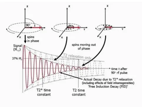
Figure 2.3 –Transversal magnetization relaxation, after a 90° RF pulse is applied at equilibrium. Initially the transverse magnetisation (red arrow) has a maximum amplitude as the population of proton’s spin magnetic moments rotate in phase. The amplitude of the net transverse magnetisation decays as the proton’s spin magnetic moments move out of phase with one another (shown by the small black arrows). The resultant decaying signal is known as the Free Induction Decay (FID). The overall term for the observed loss of phase coherence (de-phasing) is T2* relaxation, which combines the effect of T2 relaxation and additional de-phasing caused by local variations (inhomogeneities) in the applied magnetic field. T2 relaxation is the result of spin-spin interactions and due to the random nature of molecular motion, this process is irreversible. T2* relaxation accounts for the more rapid decay of the FID signal, however the additional decay caused by field inhomogeneities can be reversed by the application of a 180° refocusing pulse. Both T2 and T2* are exponential processes with times constants T2 and T2* respectively. This is the time at which the magnetization has decayed to 37% of its initial value immediately after the 90° RF pulse. Image adapted from (Ridgway, 2010). ... 31

Figure 2.4 – Schematization of Spin-Echo sequence. The presence of magnetic field inhomogeneities causes additional de-phasing of the proton magnetic moments. The Larmor frequency is slower where the magnetic field is reduced and faster where the field is increased resulting in a loss or gain in relative phase respectively. After a period of half the echo time, TE/2, the application of a 180° RF pulse causes an instantaneous change in sign of the phase shifts by rotating the spins (in this example) about the y axis. As the differences in Larmor frequency remain unchanged, the proton magnetic moments the move back into phase over a similar time period, reversing the de-phasing effect of the magnetic field inhomogeneities to generate a spin echo. In addition to the effect of the 180° refocusing pulse, gradients are applied to de-phase and re-phase the signal for imaging purposes. Note that for spin echo pulse sequences, the second gradient has the same sign as the first, as the 180° pulse also changes the sign of the phase shifts caused by the first gradient. Image adapted from (Ridgway, 2010). ... 32

Figure 2.5 – Schematization of Gradient-Echo sequence. The application of the 1st positive magnetic field gradient causes rapid de-phasing of the transverse magnetisation, Mxy. Therefore the FID signal to zero amplitude. The application of the 2nd negative magnetic field gradient reverses the de-phasing caused by the first gradient pulse, resulting in recovery

of the FID signal to generate a gradient echo at the echo time, TE. Extension of the time duration of the second gradient to twice that of the first gradient causes the FID to then de-phase to zero. The maximum amplitude of the echo depends

on both the T2* relaxation rate and the chosen TE. Image adapted from (Ridgway, 2010). ... 33

Figure 2.6 – Schematization of biological diffusion. Free water diffusion in extracellular mediums (left) and water diffusion in fibrous tissues (right). In first medium (left) in absence of boundaries the movement of the molecules is not constrained; in fact, at the molecular level the diffusion of water is random. On other hand, the boundaries (right) constrain the movement of the molecules and its movement is orientated in the direction of the fibres. Image adapted from (Winston, 2012). ... 35

Figure 2.7 – Representation of PGSE pulse sequence. G corresponds to the amplitude of the gradient applied during the time δ. The ∆ represents the time between pulses and the TE corresponds to the total time – Echo time. Image adapted from (Winston, 2012). ... 36

Figure 3. 1 – Schematization of the model applied by Moorhead et al., to correct the variability between scanners. Image adapted from (Moorhead et al., 2009). ... 47

Figure 4.1 – Coefficient of Variation expressed as a percentage value for each type of image analysed. Each bar represents the mean COV value for each centre. The line corresponds to the standard deviation of the COV value. ... 53

Figure 4.2 – Coefficient of Variation expressed as a percentage value for FA images. Each bar represents the mean COV value for each ROI in the three centres. ... 54

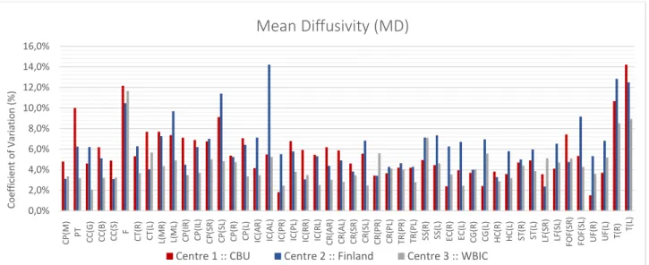
Figure 4.4 – Coefficient of Variation expressed as a percentage value for MD images. ... 54

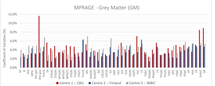
Figure 4.4 – Coefficient of Variation expressed as a percentage value for GM images. ... 55

Figure 4.5 – Coefficient of Variation expressed as a percentage value for MD images. ... 55

Figure 4.6 – Summary of the analysis performed for the 48 ROI defined. The red stars correspond to the values defined statistically as outliers. ... 56

Figure 4.7 – Coefficient of Variation expressed as a percentage value for each type of image analysed. Each bar represents the mean COV value. The line corresponds to the standard error of the COV value. ... 57

Figure 4.8 – Coefficient of Variation expressed as a percentage value for FA images. Each bar represents the mean COV value for each ROI across centres. ... 58

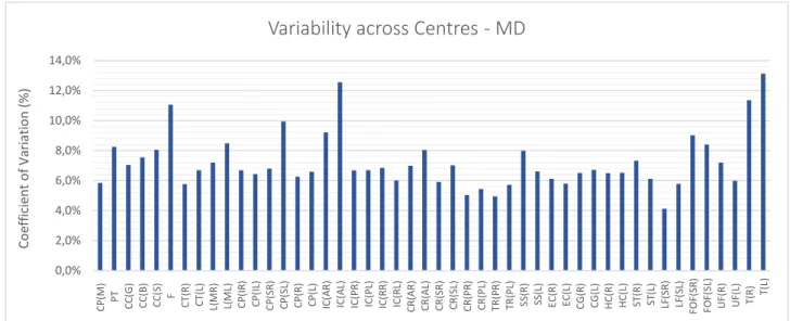
Figure 4.9 – Coefficient of Variation expressed as a percentage value for MD images for each ROI across centres. .. 58

Figure 4.10 – Coefficient of Variation expressed as a percentage value for GM images across centres. ... 58

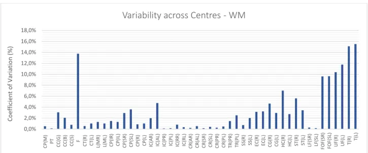
Figure 4.11 – Coefficient of Variation expressed as a percentage value for WM images for each ROI across centres. ... 59

Figure 4.12 – Summary of the analysis performed for the 48 ROI defined. The red starts correspond to the values defined statistically as outliers. ... 59

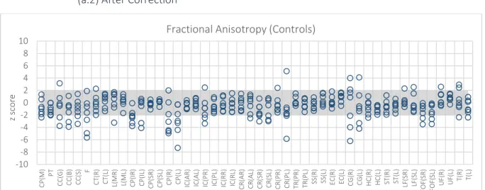
Figure 5.1 –FA maps. Z score of the Controls from Centre 3 – WBIC – when expressed in terms of controls from Centre 2 - Finland. The shadow region corresponds to the region of non-significant differences among subjects. Each circle represents a different subject. ... 65

Figure 5.2 – FA maps. Z score of the Patients when expressed in terms of a baseline defined by the controls from the two centres under study. ... 66

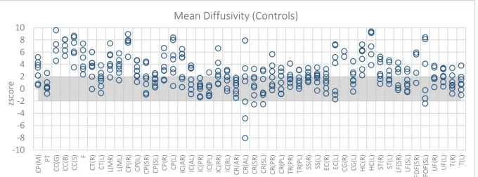
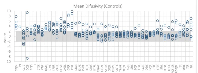
Figure 5.3 – MD maps. Z score of the Controls from Centre 3 – WBIC – when expressed in terms of controls from

Centre 2 - Finland. ... 66

Figure 5.4 – MD maps. Z score of the Patients for the Mean Diffusivity data. ... 66

Figure 5.5 – GM maps. Z score of the Controls from Centre 3 – WBIC – when expressed in terms of controls from Centre 2 – Finland. ... 67

Figure 5.6 – GM maps. Z score of the Patients when expressed in terms of a baseline defined by the controls from the two centres under study. ... 67

Figure 5.7 – WM maps. Z score of the Controls from Centre 3 – WBIC – when expressed in terms of controls from Centre 2 - Finland. ... 67

Figure 5.8 – WM maps. Z score of the Patients when expressed in terms of a baseline defined by the controls from the two centres under study. ... 68

Figure 5.9 – FA maps. Z score of the Controls from Centre 3 – WBIC – when expressed in terms of controls from Centre 2 - Finland... 68

Figure 5.10 – FA maps. Z score of the Patients when expressed in terms of a baseline defined by the controls from the two centres under study, after correction. ... 68

Figure 5.11 – MD maps. Z score of the Controls from Centre 3 – WBIC – when expressed in terms of controls from Centre 2 - Finland. ... 69

Figure 5.12 – MD maps. Z score of the Patients when expressed in terms of a baseline defined by the controls from the two centres under study. ... 69

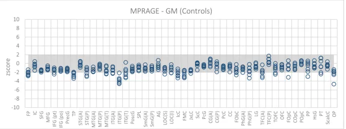
Figure 5.13 – GM maps. Z score of the Controls from Centre 3 – WBIC – when expressed in terms of controls from Centre 2 - Finland. The correction was performed using a FWHM=2mm. ... 69

Figure 5.14 – GM maps. Z score of the Patients when expressed in terms of a baseline defined by the controls from the two centres under study. The FWHM used was 2mm. ... 70

Figure 5.15 – GM maps. Z score of the Controls from Centre 3 – WBIC – when expressed in terms of controls from Centre 2 - Finland. The correction applied a FWHM=8mm. ... 70

Figure 5.16 – GM maps. Z score of the Patients when expressed in terms of a baseline defined by the controls from the two centres under study. The factor used in spatial filtering was FWHM= 8mm. ... 70

Figure 5.17 – WM maps. Z score of the Controls from Centre 3 – WBIC – when expressed in terms of controls from Centre 2 - Finland. The FWHM used was equal to 2 mm. ... 71

Figure 5.18 – WM maps. Z score of the Patients when expressed in terms of a baseline defined by the controls from the two centres under study. The correction was performed using a FWHM=2mm. ... 71

Figure 5.19 – WM maps. Z score of the Controls from Centre 3 – WBIC – when expressed in terms of controls from Centre 2 - Finland. The correction was performed using a FWHM=8mm. ... 71

Figure 5.20 – WM maps. Z score of the Patients when expressed in terms of a baseline defined by the controls from the two centres under study. The FWHM value used was 8mm. ... 72

Figure 5.21 – Number of controls significantly different for each ROI before and after correction for FA maps. ... 72

Figure 5.22 – Number of patients significantly different for each ROI before and after correction for FA maps. ... 73

Figure 5.24 – Number of patients significantly different for each ROI before and after correction for MD maps... 73 Figure 5.25 – Number of controls significantly different for each ROI before and after correction, Considering to the two types of correction applied, for GM maps. ... 74

Figure 5.26 – Number of patients significantly different for each ROI before and after correction, considering the correction A and B applied, for GM maps. ... 74

Figure 5.27 – Number of controls significantly different for each ROI before and after correction, considering the correction A and B applied, for WM maps. ... 74

Figure 5.28 – Number of patients significantly different for each ROI before and after correction, considering the correction A and B applied, for WM maps. ... 75

Figure 5.29 – Evaluation of differences for FA maps displaying voxels with significant differences between centres. The top row corresponds to the FA slices before any correction, and the bottom row corresponds to the FA slices after correction. ... 75

Figure 5.30 – Evaluation of differences for MD maps. Voxels with significant differences between centres. The top row corresponds to the MD slices before any correction, and the bottom row corresponds to the MD slices after correction. ... 76 Figure 5.31 – Evaluation of differences for GM maps. Voxels with significant differences between centres. The top row corresponds to the GM slices before any correction, and the bottom row correspond to the GM slices after correction A. ... 76

Figure 8.1 – Schematization of the mixed model to correct the variability. ... 93 Figure B.1 – Coefficient of Variation for FA maps. It is shown three different views (coronal, axial and sagittal) of the brain, in which a median value of COV for each voxel, obtained for each Centre, is represented using a colour code: red-yellow. ... c Figure B.2 – Coefficient of Variation for MD maps. It is shown three different views (coronal, axial and sagittal) of the brain, in which a median value of COV for each voxel, obtained for each Centre, is represented using a colour code: red-yellow. ... ci Figure B.3 – Coefficient of Variation for GM maps. It is shown three different views (coronal, axial and sagittal) of the brain, in which a median value of COV for each voxel, obtained for each Centre, is represented using a colour code: red-yellow. ... ci Figure B.4 – Coefficient of Variation for WM maps. It is shown three different views (coronal, axial and sagittal) of the brain, in which a median value of COV for each voxel, obtained for each Centre, is represented using a colour code: red-yellow. ... cii Figure B.5 – Coefficient of Variation for FA maps. It is shown three different views (coronal, axial and sagittal) of the brain, in which a median value of COV for each ROI, obtained for each Centre, is represented using a colour code: red-yellow. ... cii Figure B.6 – Coefficient of Variation for MD maps. It is shown three different views (coronal, axial and sagittal) of the brain, in which a median value of COV for each ROI, obtained for each Centre, is represented using a colour code: red-yellow. ... ciii

Figure B.7 – Coefficient of Variation for GM maps. It is shown three different views (coronal, axial and sagittal) of the brain, in which a median value of COV for each ROI, obtained for each Centre, is represented using a colour code: red-yellow. ... ciii Figure B.8 – Coefficient of Variation for FA maps. It is shown three different views (coronal, axial and sagittal) of the brain, in which a median value of COV for each ROI, obtained for each Centre, is represented using a colour code: red-yellow. ... civ Figure C.1 – Number of Patients significantly different when compared with the baseline, for each ROI, before and after correction. ... cv

Figure C.2 – Number of Patients significantly different when compared with the baseline from centre 3, before and after correction. ... cvi

Figure C.3 – Number of Patients significantly different when compared with the baseline from centre 2, before and after correction. ... cvi

Figure C.4 – Number of Patients significantly different when compared with the baseline from centre 3, before and after correction. ... cvi

Figure C.5 – Number of Patients significantly different when compared with the baseline from centre 2, before and after the two types of corrections were applied. ... cvii

Figure C.6 – Number of Patients significantly different when compared with the baseline from centre 3, before and after the two types of corrections were applied. ... cvii

Figure C.7 – Number of Patients significantly different when compared with the baseline from centre 2, before and after the two types of corrections were applied. ...cviii

Figure C.8 – Number of Patients significantly different when compared with the baseline from centre 3, before and after the two types of corrections were applied. ...cviii

Figure D.1 – In both panels a b0 volume is shown in the axial plane, visualized with a window of intensities [3; 1500]. Panel A shows the b0 volume from one of the subjects without spatial filtering. Panel B shows the result of spatial filtering using smoothing by a Gaussian kernel with FWHM=2mm... cx

L

IST OF

T

ABLES

Table 4.1 – Summary of the Coefficient of Variation obtained in within centre. ... 56 Table 4.2 - Summary of the Coefficient of Variation obtained across centres. ... 60 Table 5.1 – Summary of statistical analysis.. ... 77 Table 6.1 – SVM results of the data classification of the results of model correction, in terms of the Centre. ... 85 Table 7.1 – SVM results of the data classification of the results of models of correction, in terms of the Centre. ... 89

L

IST OF

A

BREVIATIONS

ANCOVA Analysis of Covariance

CBU Cognition and Brain Sciences Unit

COV Coefficient of Variation

CT Computerized Tomography

DTI Diffusion Tensor Imaging

DWI Diffusion Weight Imaging

EPI Echo Planar Imaging

FA Fractional Anisotropy

FID Free Induction Decay

FLIRT FMRIB's Linear Image Registration Tool

fMRI Functional Magnetic Resonance Imaging

FNIRT FMRIB's Non Linear Image Registration Tool

FOV Field of View

FSL FMRIB Software Library

FWHM Full Width at Half Maximum

GCS Glasgow Coma Scale

GE Gradient Echo Sequence

GLM General Linear Model

GM Grey Matter

GPR Gaussian Process Regression

ICC Interclass Correlation Coefficient

JHU Johns Hopkins University

LLS Linear Least Squares

LOC Loss of Conscientious

MD Mean Diffusion

MPRAGE Magnetization Prepared Rapid Gradient Echo Sequence

MRI Magnetic Resonance Imaging

MT Magnetization Transfer

NLLS Non-Linear Least Squares

PD Proton Diffusion

PGSE Pulsed-Gradient Spin-Echo Sequence

ROI Region of Interest

SE Spin Echo Sequence

SFNR Signal-to-Fluctuation-Noise-Ratio

sMRI Structural Magnetic Resonance Imaging

SNR Signal-to-Noise-Ratio

SVM Support Vector Machine

TBI Traumatic Brain Injury

TBSS Tract-Based Spatial Statistics

VBM Voxel-based morphometry

WBIC Wolfson Brain Imaging Centre

Chapter 1

I

NTRODUCTION

1.1. C

The World Health Organization expects that Traumatic Brain Injury will surpass many diseases as the major cause of death and disability by the year 2020 (Hyder, Wunderlich, Puvanachandra, & Gururaj, 2007). In Europe, TBI affects about 7.7 million individuals, and it is estimated that 30-70% of them will suffer on-going mental illness as well physical and cognitive disabilities (Kostro et al., 2014; Wilson et al., 2014)

Traumatic Brain Injury (TBI) is defined as an alteration in brain function, or other evidence of brain pathology, caused by an external factor (Menon, Schwab, Wright, & Maas, 2010). TBI can be classified as mild, moderate or severe based on acute TBI variables that include the following clinical signs:

● Duration of loss of consciousness (LOC);

● Glasgow Coma Score (GCS);

● Loss of memory for events immediately before or after the injury (Post Traumatic Amnesia - PTA);

● Neurologic deficits, such as weakness, loss of balance, dysphasia paresis/plegia, sensory loss, aphasia, etc.

The most common manifestation of this pathology is mild TBI, with an incidence of 70-90% of all cases. (Kraus et al., 2007)

Certain brain regions are more susceptible to contusion following TBI, such as frontal and anterior temporal cortices, due to the proximity to the skull. On the other hand, white matter tracts are particularly susceptible to the shearing forces that occur with TBI. (Risdall & Menon, 2011)

The diagnosis of TBI is made when the symptoms and signs are closely related to the insult. However, other clinical manifestations may be delayed. These manifestations include cognitive changes such as decreased mental flexibility, impaired attention, poor planning, impaired judgement, deficits in verbal fluency, problems with working memory as well as increased impulsivity (Kraus et al., 2007). Determining the extent of clinically relevant neuropathology associated with TBI might be problematic. To solve this issue, modern medical imaging techniques have been used, such as Diffusion Tensor Imaging (DTI). These MRI techniques provide pathological information in vivo. Besides, the prospect of tracking white matter microstructural changes over time holds the promise of measuring neuroplasticity and repair following TBI, which can provide a way of monitoring the therapeutic response and can improve the efficiency of the treatment.

However, regarding the inherent heterogeneity of TBI, which is determined by multiple factors1_{, the study of this} pathology is a huge challenge, which requires a diversified dataset. A large dataset ensures the presence of a large spectrum of different symptoms and of therapeutic responses, allowing a more complete understanding of this illness. Thus, the multicentre studies have proven themselves very useful to collect data from subjects with interesting characteristics for TBI research, contributing to increase the statistical power of the TBI studies and to improve the reliability of the assumptions made about this illness.

Considering this fact, a pragmatic approach to TBI research is required. The CENTER-TBI Project is a large European study that aims to improve the care for patients with TBI (Figure 1.1.). It consists in a prospective longitudinal observational study in 60 centres from 20 countries including approximately 5400 patients, and it forms part of the larger global initiative InTBIR: International Initiative for Traumatic Brain Injury Research with projects currently ongoing in Europe, the US and Canada.

The main goals of the CENTER-TBI are the improvement of the characterization of TBI as a disease and the identification of the most effective clinical interventions for managing TBI. For that, the CENTER-TBI study will include works in several areas of research, such as neuroinformatics, genetic associations, MR imaging, biomarkers and comparative effectiveness research (CER), which will give a complete and detailed characterization of TBI (CENTER-TBI, 2014).

The CENTER-TBI purposes to connect the real clinical situation to the approaches studied, in order to translate the research outputs into valid and useful information for physicians and clinicians, allowing a better care of the patients, as well as a more efficient approach for the hospitals and health care centres. Therefore, it will develop and sustain an international TBI knowledge community that integrates results of the project with high quality 'living evidence reviews' of the current state of knowledge.

These goals will only be possible if the reliability of the study is ensured. It is in this topic that the project that foments this thesis is inserted. The main goals of the thesis will be discuss in the next section.

1.2.

O

D

The principal aim of this thesis is to develop robust methods for quantification and correction of variability across scanners in multicentre studies. Secondly, this dissertation is inserted in the CENTER-TBI Project and, consequently, it aims to show the potential of multicentre studies for the improvement of diagnosis of TBI, and as an advanced method in brain study.

Also, it is expected that this work can be part of the set of published studies in the context of CENTER-TBI, specifically as a study of the impact of the variation introduced by the scanner in multicentre studies and contributing to the definition of which methodologies could be useful to overcome the main issues behind these studies.

1_{The factors which contribute to the heterogeneity of TBI are injury location, physiology, extracranial injuries, and constitutional effects}

1.3. O

D

In the present chapter, Chapter 1, a brief contextualization of the project, in which this dissertation is inserted, is presented. In this chapter, the goals of the project are detailed.

The second chapter introduces the concepts behind medical imaging useful for TBI analysis, namely MRI. Considering the topics presented, the chapter is divided into two sections. In the first one, the concepts on MRI, such as the physical principles and imaging reconstruction principles of MRI, are described.

Chapter 3 introduces the state of the art of multicentre studies. The limitations and advantages of multicentre studies, as well as their usefulness on TBI study, are explained. In this chapter, the methodologies applied in previous studies to quantify the variability introduced by the hardware in medical imaging are also detailed, and the impact this variability on the studies reliability and data reproducibility is also discussed. A set of strategies for data calibration and error correction presented in the literature are described in the last section of this chapter.

In Chapter 4 the dataset used in study developed on context of this dissertation and its main characteristics are detailed. The methods used to quantify the variability between scanners and intra-scanner are also described in this chapter. In addition, the variation measured intra- and inter-centre is presented as well as a comment about the values achieved for the three centres, independently, and for the inter-centre analysis.

The following chapters, Chapters 5 and 6, a comprehensive and extensive description of the methods used for the elimination of the variability are presented as well as the main results obtained using the models employed. Thereby, in Chapter 5 an evaluation of the Spatial Filtering Model is presented, in which an ROI analysis and a voxel based analysis are compared and discussed. In this chapter, the effectiveness of a default pipeline to correct for the errors in Magnetization Prepared Rapid Gradient Echo (MPRAGE) images, namely in Grey Matter (GM) and White Matter (WM) segmentations is also discussed. In Chapter 6, the usefulness of using covariates to absorb the error introduced by nuisance variables in the data is discussed.

In Chapter 7 a comparison between models is presented.

Finally, Chapter 8 presents a conclusion and evaluation of the project. Moreover, in this chapter, an overview of the work developed as well as a reflection on future work in the context of multicentre studies and variability correction in MRI are presented.

Chapter 2

B

ACKGROUND

2.1. I

In medical science when we refer to medical imaging, we are referring to a wide range of techniques and technologies which are used to analyse the human body for purposes of diagnosis, monitoring or treating pathological medical conditions.

Medical imaging includes a range of non-invasive techniques which have been proven to be an essential tool for current medical practice. These techniques are part of the current approach to diagnose and evaluate patients when they arrive at a medical facility or hospital. In fact, medical imaging techniques enable higher viability and accuracy of diagnosis, which result in greater effectiveness of medical treatment. The use of medical imaging has enabled physicians to study the symptoms and progress of a specific pathology, without the need for exploratory surgery. In modern medicine, there are several medical imaging methods with different features, which register different types of information that may be more targeted to functional or anatomical details, depending on the specific symptoms or pathology. For instance, techniques like structural Magnetic Resonance Imaging (sMRI), Computerised Tomography (CT) or Diffusion Tensor Imaging (DTI) are more directed to anatomical studies, whereas functional Magnetic Resonance Imaging (fMRI) is useful in functional evaluations.

Nowadays, medical imaging techniques are an important procedure in the employed methodology to study the patho-physicological mechanisms of several diseases, and at the same time ensuring the comfort and safety of the individuals being analysed. Thereby, taking all characteristics into account it is obvious why these techniques have achieved such an important role in fields such as Clinical Neuroscience. In particular, medical imaging methods like standard MRI structural images can readily demonstrate large focal contusions or bleeds, diffuse axonal injury may be detected indirectly by brain volume loss (volumetric analysis) (Boven et al., 2011). On the other hand, studies using functional MRI (fMRI) in patients with TBI show abnormal patterns of brain activation in patients compared with healthy control subjects (Boven et al., 2011). DTI also demonstrated potential in TBI diagnosis, since DTI allows for the specific examination of the integrity of white matter tracts, which are especially vulnerable to the mechanical trauma of TBI (Kraus et al., 2007; Shenton et al., 2012). Thereby, there has been increasing interest in using MRI techniques to diagnose and monitor TBI patients (Risdall & Menon, 2011; Shenton et al., 2012).

In this chapter the basic principles of MRI and DTI are presented, and the advantages and limitations of these techniques for the purpose of medical diagnostics are discussed.

2.2. M

I

2.2.1. Magnetic Resonance Imaging

Magnetic Resonance Imaging (MRI) is a non-invasive technique which allows in-vivo imaging of the human body, without requiring the use of radiation. MRI is a high resolution technique and it is frequently used to acquire brain images, since it allows acquisition of images with high level of anatomical detail and, consequently, makes possible the detection and monitoring of many lesions.

(a) Physical principles behind MRI

MRI uses magnetic fields and electromagnetic energy to generate signals from atomic nuclei, which can be used to create an image. The human body is composed of 60% of water, whereby the hydrogen nuclei the third most abundant in the human body. MRI uses the signal from hydrogen nuclei to generate the image; however, it is possible to image other nuclei such as sodium.

When a volume of water, in this case a body area, is exposed to an external and static magnetic field, B0, the spin’s

magnetic moment (𝜇⃗) of the protons aligns in the direction of B0 (Figure 2.1).

Figure 2. 1 – External magnetic field effect on protons. In the left side of the image is possible to see the protons in absence of magnetic field. In consequence, the spin’s magnetic moment of the protons are not aligned (represented by the black arrows). On other hand, when a magnetic field is applied (right side) the spin’s magnetic moment of the protons aligns in direction of B0. The orientation of the

spins is explained by the Boltzmann statistics, which explains the different orientation of the spin’s magnetic momentum of protons represented at this image. Image adapted from (Haacke, E. M; Brown, R.W; Thompson, M. R; Venkatesan, 1999).

This phenomenon is explained by Boltzmann statistics, which state that there are more spins in the lower energy level (orientated parallel to B0), than spins in the higher energy level (orientated anti-parallel to B0). In this situation, the spin’s

magnetic moment starts precessing at a specific frequency, known as the Larmor frequency – ω0:

𝜔0= 𝛾𝐵0 Equation 2.1.

where 𝛾 is the gyromagnetic ratio.

The sum of magnetic moments of all the protons exposed to the external magnetic field is given by the Net Magnetic Moment (𝑀⃗⃗⃗), which is aligned with B0. This vector has a component in the B0 direction, designated as longitudinal

as transversal magnetization (Mxy) is close to zero at this state. Note that, in this situation, the protons are not precessing

in phase and the 𝜇⃗ component transversal to B0 is randomly distributed.

By applying a radio frequency pulse, with the Larmor frequency, it is possible to force the protons to precess in phase, which will increase the Mxy. The angle of rotation relative to the main magnetic field direction is called flip angle. When the

radio frequency pulse is interrupted the 𝑀⃗⃗⃗ starts losing its transverse component, and returns to the equilibrium state. This effect of relaxation can be induced by two different processes: the spin-lattice relaxation (T1 relaxation) or a spin-spin interaction (T2 relaxation). In the first case (Figure 2.2), the protons transfer their energy to the surrounding macro-molecules and realign with B0. T1 is the time constant that represents the time required for the protons to recover 63% of initial Mz component, after a 90 degrees pulse has been applied. This phenomenon can be described by the following

expression:

𝑀𝑧(𝑡) = 𝑀0[1 − exp(

−𝑡 𝑇1

)] Equation 2.2.

where 𝑀0 refers to the magnetization in the equilibrium state.

Figure 2.2 – Proton relaxation and longitudinal magnetization recovery, after a 90° RF pulse is applied at equilibrium. The z component of the net magnetisation, Mz, is reduced to zero. This component recovers gradually back to its equilibrium value if no further RF pulses are applied. The recovery of Mz is an exponential process with a time constant T1. This is the time at which the magnetization has recovered to 63% of its value at equilibrium. Image adapted from (Ridgway, 2010).

In the second case, (Figure 2.3), the reduction of Mxy is a consequence of loss of phase coherence between the

protons, which can be expressed by Equation 2.3, where Mxy0 refers to the initial transversal magnetization and T2 corresponds to the time constant of spin-spin relaxation.

𝑀𝑥𝑦0(𝑡) = 𝑀𝑥𝑦0[exp(

−𝑡 𝑇2

Figure 2.3 –Transverse magnetization relaxation, after a 90° RF pulse is applied at equilibrium. Initially the transverse magnetisation (red arrow) has a maximum amplitude as the population of proton’s spin magnetic moments rotate in phase. The amplitude of the net transverse magnetisation decays as the proton’s spin magnetic moments move out of phase with one another (shown by the small black arrows). The resultant decaying signal is known as the Free Induction Decay (FID). The overall term for the observed loss of phase coherence (de-phasing) is T2* relaxation, which combines the effect of T2 relaxation and additional de-phasing caused by local variations (inhomogeneities) in the applied magnetic field. T2 relaxation is the result of spin-spin interactions and due to the random nature of molecular motion, this process is irreversible. T2* relaxation accounts for the more rapid decay of the FID signal, however the additional decay caused by field inhomogeneities can be reversed by the application of a 180° refocusing pulse. Both T2 and T2* are exponential processes with times constants T2 and T2* respectively. This is the time at which the magnetization has decayed to 37% of its initial value immediately after the 90° RF pulse. Image adapted from (Ridgway, 2010).

(b) Image Principles and Imaging sequences

During both relaxation processes, the protons emit a radio frequency with the Larmor frequency, which is designated as free induction decay (FID). Considering that the FID does not provide a spatial discrimination, for image generation it is necessary to apply a position encoding process.

When a radio frequency pulse is applied with a specific bandwidth, only the protons with Larmor frequency coinciding with the RF pulse frequency profile are excited, which allows for a single slice to be selected. However, this procedure does not differentiate the protons within the same slice. For that, it is necessary to apply two more gradients in the orthogonal plane to the slices selected. By applying these gradients, and measuring the echoes produced, it is possible to fill the k-space2_{, with information that codifies the spatial positions in the image according to their frequency. The spatial} information can be obtained applying a Fourier transform to the k-space.

2 _{Thek-space refers to a matrix composed by complex values, which are sampled during an MR acquisition, in a premeditated}

scheme controlled by apulse sequence, i.e. an accurately timed sequence of radiofrequency and gradient pulses. Therefore, the k-space can be described as atemporary image space, in which data from digitized MR signals are stored during data acquisition. In fact, the k-space holdsrawdata beforereconstruction. The k-space corresponds tothespatial frequencydomain, and can be described using the frequency encoding component (kFE) and the phase encoding component (kPE) components, which can be expressed using the following

expressions: 𝑘𝐹𝐸=𝛾𝐺𝐹𝐸𝑚∆𝑡 and 𝑘𝑃𝐸=𝛾𝑛𝐺𝑃𝐸𝜏. The ∆𝑡 corresponds to the interval of time during the sample is acquired, 𝜏 is the

MRI allows the acquisition of images with different contrast by changing the RF pulse and gradient design throughout time. Each combination of RF and gradient steps is called an MR sequence. The Spin-Echo sequence is one of the most often used to acquire MRI images (Figure 2.4). The gradient-echo sequence is another kind of sequence commonly used (Figure 2.5), which is characterized by shorter acquisition times compared to Spin-Echo. In this project, images acquired using a magnetization prepared rapid gradient echo sequence (MPRAGE) were analysed. In this case, the sequence starts with magnetization preparation to introduce a T1 contrast. This is achieved using an RF pulse with a flip angle of 180 degrees, also denominated as inversion pulse. Mz is described now by the Equation 2.4, instead of the Equation 2.2.

Figure 2.4 – Schematization of Spin-Echo sequence. The presence of magnetic field inhomogeneities causes additional de-phasing of the proton magnetic moments. The Larmor frequency is slower where the magnetic field is reduced and faster where the field is increased resulting in a loss or gain in relative phase respectively. After a period of half the echo time, TE/2, the application of a 180° RF pulse causes an instantaneous change in sign of the phase shifts by rotating the spins (in this example) about the y axis. As the differences in Larmor frequency remain unchanged, the proton magnetic moments move back into phase over a similar time period, reversing the de-phasing effect of the magnetic field inhomogeneities to generate a spin echo. In addition to the effect of the 180° refocusing pulse, gradients are applied to de-phase and re-phase the signal for imaging purposes. Note that for spin echo pulse sequences, the second gradient has the same sign as the first, as the 180° pulse also changes the sign of the phase shifts caused by the first gradient.Image adapted from (Ridgway, 2010).

the 2D-Fourier Transform of this encoded signal results in a representation of the spin density distribution in two dimensions. Thus position (x,y) and spatial frequency (kFE, kPE ) constitute a Fourier transform pair (Twieg, 1983)

Figure 2.5 – Schematization of Gradient-Echo sequence. The application of the 1st positive magnetic field gradient causes rapid de-phasing of the transverse magnetisation, Mxy. Therefore the FID signal tends to zero amplitude. The application of the 2nd negative magnetic field gradient reverses the de-phasing caused by the first gradient pulse, resulting in recovery of the FID signal to generate a gradient echo at the echo time, TE. Extension of the time duration of the second gradient to twice that of the first gradient causes the FID to then de-phase to zero. The maximum amplitude of the echo depends on both the T2* relaxation rate and the chosen TE.Image adapted from (Ridgway, 2010).

The T1 contrast will dominate the sequence, depending on the time between the inversion pulse and the gradient echo sequence. The period of time between both sequence periods is called inversion time TI. Then, when the Gradient Echo (GE) sequence is applied the signal is acquired. This acquisition period is followed by a magnetization recovery period where the magnetization recovers during a delay time (t) before the next inversion pulse, in order to prevent saturation effects.

𝑀𝑧(𝑡) = 𝑀0[1 − 2exp(

−𝑡 𝑇1

)] Equation 2.4.

2.2.2. Diffusion Tensor Imaging

Diffusion Tensor Imaging (DTI) is a medical imaging technique that exploits the exquisite sensitivity of magnetic resonance imaging to diffusion processes to measure microscopic tissue orientation characteristics in vivo (Williams, Paul, Clark, & Gordon, 2007).

DTI characterizes the three-dimensional diffusion of water as a function of spatial localization. This technique is highly sensitive to the microstructural architecture of brain tissues, allowing the assessment of changes in the diffusion pattern in the presence of pathological symptoms (Alexander, Lee, Lazar, & Field, 2008).

The methods used to acquire and analyse DTI have evolved significantly in the last years. Among these are new pulse sequences and diffusion tensor encoding schemes that improve the accuracy and spatial resolution, by reducing the artefacts in tensor measurements.

(c) Physical principles of Diffusion

Diffusion is a kinetic process, in particular a mass process, which occurs in a fluid that leads to the homogenization, or uniform mixing, of the chemical components in a phase (Ceric, 2005).

The process of diffusion depends on many factors such as size and form of particles diffused, temperature and viscosity of the fluid. The Fick Law describes the flux, J, (Equation 2.5) of mass or energy in a medium where there isn’t an initial thermic and chemical balance (Equation 2.6). Note that D denotes the diffusion coefficient and 𝛻C is the concentration gradient of the diffusing component.

𝐽 = −𝐷𝛻𝐶 Equation 2.5. 𝐽𝑥 = −𝐷 𝜕𝐶 𝜕𝑥 ; 𝐽𝑦= −𝐷 𝜕𝐶 𝜕𝑦; 𝐽𝑧= −𝐷 𝜕𝐶 𝜕𝑧 Equation 2.6.

The movement of particles between two compartments due to diffusion processes results in a decrease of the concentration gradient, reaching a steady state, in which a uniform concentration across the medium is achieved. Considering the principle of mass conservation, described by Equation 2.7 where r represent a space vector (x,y,z) and t the temporal component, and using Fick’s first law (Equation 2.5), it is possible to obtain Fick’s second law, that describes the variation of concentration in a medium (Equation 2.8) (Ceric, 2005).

𝛻𝐽(𝑟, 𝑡) = −𝜕𝐶(𝑟, 𝑡) 𝜕𝑡 Equation 2.8. 𝐷𝛻2_{𝐶(𝑟, 𝑡) =}𝜕𝐶(𝑟, 𝑡) 𝜕𝑡 Equation 2.9.

On a molecular level, diffusion refers to a random displacement of the molecules agitated by thermal energy, known as Brownian motion (Hagmann et al., 2006).

Einstein described the diffusion coefficient, D, as a proportion of the mean squared-displacement divided by the number of dimensions, n, and the interval of time needed to the diffusion process, ∆𝑡 (Equation 2.9). (Einstein, 1956)

𝐷 =〈∆𝑟

2_〉

2𝑛∆𝑡

Equation 2.9.

In the absence of boundaries, the diffusion of water, on a molecular level, is described by a Gaussian probability density, as shown in the following equation:

𝑃(∆𝑟, ∆𝑡) = 1

√(4𝜋𝐷∆𝑡)3× exp (

−∆𝑟2

4𝐷∆𝑡)

(d) Biological Diffusion

The water diffusion in biological tissues occurs inside, outside and trough cellular structures, and it is modulated by the interactions with cellular membranes and organelles. The cellular membranes show a behaviour similar to boundaries dividing compartments. Due to this fact, the intracellular water tends to be more restricted when compared with extracellular water and, consequently, has a restricted diffusion. In the case of fibrous tissues, such as white matter, the water diffusion is highly restricted in the directions perpendicular to the fibres and, on the contrary, shows high diffusion in the directions parallel to the fibre orientation, as is schematized in Figure 2.6 (Alexander et al., 2008; Winston, 2012). Therefore, the diffusion in fibrous tissues can be considered to be anisotropic.

Figure 2.6 – Schematization of biological diffusion. Free water diffusion in extracellular mediums (left) and water diffusion in fibrous tissues (right). In first medium (left) in absence of boundaries the movement of the molecules is not constrained; in fact, at the molecular level the diffusion of water is random. On other hand, the boundaries (right) constrain the movement of the molecules and its movement is orientated in the direction of the fibres. Image adapted from (Winston, 2012).

Basser et al, (Basser, PJ; Matitello, J; LeBihan, 1994), described the anisotropic diffusion behaviour using the diffusion tensor (Equations 2.11), which is a 3x3 covariance matrix (Equation 2.12) that describes the covariance of diffusion displacements in three directions.

Note, that the off-diagonal elements are symmetric about the diagonal (Dij=Dji), thus Dxy = Dyx, Dxz=Dzx, and Dyz=Dzy

and only six non-collinear diffusion encoding directions are needed. The diagonal elements correspond to diffusion variances along the x, y and z directions.

The diagonalization of the diffusion tensor yields the eigenvalues (λ1, λ2, and λ3) and the respective eigenvectors (ê1,

ê2 and ê3), which describe the directions and apparent diffusivities along the axes of principal diffusion. If the diffusion is

isotropic, then λ1 = λ2 = λ3, and the tensor can be visually represented by a sphere. On the other hand, if the diffusion is

anisotropic then λ1 > λ2 > λ3, and the tensor assumes an ellipsoid format (Alexander et al., 2008).

𝑃(∆𝒓, ∆𝑡) = 1 √(4𝜋∆𝑡)3_|𝑫|× exp ( −∆𝒓𝑻_𝑫−𝟏_∆𝒓 4∆𝑡 ) Equation 2.11. 𝐷 = [ 𝐷𝑥𝑥 𝐷𝑥𝑦 𝐷𝑥𝑧 𝐷𝑦𝑥 𝐷𝑦𝑦 𝐷𝑦𝑧 𝐷𝑧𝑥 𝐷𝑧𝑦 𝐷𝑧𝑧 ] Equation 2.12.

(e) Diffusion-Weighted Imaging

The MRI sequence most commonly used to quantify the diffusion in brain is a pulsed-gradient spin-echo (PGSE) with a single shot, echo planar imaging (EPI) readout (Figure 2.7). In this sequence, the first gradient pulse de-phases the magnetization across the sample, whilst the second pulse is responsible for re-phasing the magnetization. In the case of static molecules (molecules that are not diffusing), the phases induced by both gradient pulses will completely cancel, the magnetization will be maximally coherent and, consequently, there will be no signal attenuation due to diffusion. On the other hand, in the case of diffusion motion in the gradient direction, motion will cause the signal phase to change by different amounts for each pulse and for each spin; in other words, there will be a phase difference, which is proportional to the displacement, the area of diffusion gradient pulses defined by the amplitude, G, and the duration, δ, and the spacing between pulses, ∆. Therefore, the phase dispersion due to diffusion will cause signal attenuation.

Figure 2.7 – Representation of PGSE pulse sequence. G corresponds to the amplitude of the gradient applied during the time δ. The ∆ represents the time between pulses and the TE corresponds to the Echo time. Image adapted from (Winston, 2012).

Assuming the Gaussian displacement distribution mentioned before, the amplitude of the signal attenuation can be calculated with the following expression:

𝑆 = 𝑆0exp {−(𝛾𝐺𝛿)2× (∆ −

𝛿 3) × 𝐷}

Equation 2.13.

where S0 is the signal without attenuation (situation where no diffusion gradient is applied), 𝛾 is the gyromagnetic ratio

and D is the diffusion coefficient. This expression can be rewritten (Equation 2.14 and 2.15), and the D coefficient can be estimated using Equation 2.16, in the particular case in which the image only has one b-value.

𝑏 = (𝛾𝐺𝛿)2_{× (∆ −}𝛿 3) Equation 2.14. 𝑆 = 𝑆0exp{−𝑏 × 𝐷} Equation 2.15. 𝐷 = −1 𝑏ln( 𝑆 𝑆0 ) Equation 2.16.

The Diffusion-weighted image (DWI) is extremely sensitive to subject motion, and even small motions can lead to phase and amplitude modulations in the acquired data and significant ghosting artefacts in the reconstructed images. Considering this fact, an EPI sequence could be useful to acquire images with a low presence of artefacts, since the fast acquisition speed of EPI turns this sequence highly efficient and maximizes the image signal-to-noise ratio. This fact reduces

the time that subjects need to be immobilized, reducing the probability of bulk motion. Thus, the EPI sequence improves the accuracy of the diffusion measurements, thereby this sequence is the most commonly used sequence to acquire DTI images. However, the EPI sequence shows some limitations, such as the image distortion caused by magnetic field inhomogeneities (Alexander et al., 2008).

(f) Diffusion Tensor Imaging

As detailed above, the anisotropic diffusion can be fully described using a diffusion tensor. Diffusion Tensor Imaging (DTI) uses the raw DWI images to estimate the diffusion tensor for all voxels in the brain (Alexander et al., 2008; Basser, PJ; Matitello, J; LeBihan, 1994).

Considering Equation 2.15, which describes the anisotropic diffusion in a medium, it is possible to define a matrix B which only depends on the parameters of the diffusion gradients (Equation 2.17), and where each entry of matrix B, bij, is estimated using Equation 2.14, taking into account the G value for position ij.

𝑩 = [ 𝑏𝑥𝑥 𝑏𝑥𝑦 𝑏𝑥𝑧 𝑏𝑦𝑥 𝑏𝑦𝑦 𝑏𝑦𝑧 𝑏𝑧𝑥 𝑏𝑧𝑦 𝑏𝑧𝑧 ] Equation 2.17.

Thus, the Equation 2.15 can be rewritten as:

𝑆 = 𝑆0exp{−𝐵. 𝐷} Equation 2.18.

A minimum of six non-collinear diffusion encoding directions are required to estimate the diffusion tensor, since the elements of the matrix D are symmetric about the diagonal. The estimation of diffusion parameters from raw DWI (using the general expression shown in Equation 2.6) can be done using a linear least square approach, denominated linear least squares (LLS), or a non-linear approach – non-linear least squares (NLLS) (Alexander et al., 2008; Winston, 2012). Note that the LLS allows to obtain a quicker solution and it is not so demanding from the computational point of view, when compared with NLLS. However, the solution obtained with LLS might be not so satisfactory, due to the propagation of errors, since in LLS the noise enters in the system as a random variable statistically dependent on the signal (Ozcan, 2011). Both approaches were implemented in this project, and their performance will be analysed in the next chapters.

The diffusion tensor can provide several DTI invariant measures, such as the mean diffusivity (MD), fractional anisotropy (FA), axial diffusivity (𝜆||) and radial diffusivity (λr).

The mean diffusivity corresponds to the trace of the diffusion tensor divided by three (Equation 2.19). This measure is proportional to the orientationally-averaged apparent diffusivity, and its values are remarkably similar across grey matter and white matter. MD is an inverse measure of the membrane density. This measure is sensitive to cellularity, edema, and necrosis. (Andrew L. Alexander, 2011). Thus, MD has an important role in the context of TBI diagnosis, since allows to evaluate the edema characteristics, which is a physical manifestation of TBI. The FA value quantifies the fraction of the whole ‘’magnitude’’ of the diffusion tensor that can be ascribed to anisotropic diffusion (Equation 2.20, the 𝜆 corresponds to the eigenvalues in the three directions defined). Finally, the axial diffusivity refers to the magnitude of diffusion along the principal ellipsoid component, so it is equal to 𝜆1. On the other hand, radial diffusivity is the mean diffusivity along

𝑀𝐷 =𝑇𝑟𝑎𝑐𝑒 (𝐷) 3 = 𝜆1+ 𝜆2+ 𝜆3 3 Equation 2.19. 𝐹𝐴 = √3 2× √(𝜆1− 〈𝜆〉)2+ (𝜆2− 〈𝜆〉)2+ (𝜆3− 〈𝜆〉)2 √𝜆12+ 𝜆22+ 𝜆23 Equation 2.20. 𝜆𝑟= 𝜆2+ 𝜆3 3 Equation 2.21.