Sistema de Controlo Inferencial com
Dispositivos Sensoriais Direcionados para o Uso
Eficiente da Água na Agricultura
JUCILENE DE MEDEIROS SIQUEIRA
ORIENTADORES:
Doutor Luís Santos Pereira
Docente Emérito
Doutora Maria Teresa Gomes Afonso do Paço
Doutor José Machado da Silva
Professor Associado
Faculdade de Engenharia
Universidade do Porto
TESE ELABORADA PARA OBTENÇÃO DO GRAU DE DOUTOR EM
ENGENHARIA DOS BIOSSISTEMAS
ii
Sistema de Controlo Inferencial com Dispositivos Sensoriais
Direcionados para o Uso Eficiente da Água na Agricultura
JUCILENE DE MEDEIROS SIQUEIRAORIENTADORES: Professor Doutor Luís Santos Pereira Professora Doutor Teresa Afonso do Paço Professor Doutor José Machado da Silva
TESE ELABORADA PARA OBTENÇÃO DO GRAU DE DOUTOR EM ENGENHARIA DOS BIOSSISTEMAS
Presidente: Doutor Ricardo Manuel de Seixas Boavida Ferreira Professor Catedrático
Instituto Superior de Agronomia Universidade de Lisboa.
Vogais: Doutora Maria Isabel Freire Ribeiro Ferreira Professora Catedrática
Instituto Superior de Agronomia Universidade de Lisboa;
Doutor Nildo da Silva Dias Professor Associado III
Universidade Federal Rural do Semi-Árido, Brasil; Doutor Aureliano Natálio Coelho Malheiro
Professor Auxiliar
Escola de Ciências Agrárias e Veterinárias Universidade de Trás-os-Montes e Alto Douro; Doutora Maria Teresa Gomes Afonso do Paço Professora Auxiliar
Instituto Superior de Agronomia Universidade de Lisboa;
Doutor João Rui Rolim Fernandes Machado Lopes Professor Auxiliar Convidado
Instituto Superior de Agronomia Universidade de Lisboa;
Doutor José Manuel Couto Silvestre Investigador Auxiliar
Instituto Nacional de Investigação Agrária e Veterinária.
Fundação CAPES- Ministério de Educação do Brasil
iii
LOW-COST OPEN SYSTEM FOR THE EFFICIENT USE OF
WATER IN ORCHARDS AND VINEYARDS
JUCILENE DE MEDEIROS SIQUEIRA
ORIENTADORES: PhD Luís Santos Pereira
PhD Teresa Afonso do Paço
PhD José Machado da Silva
TESE ELABORADA PARA OBTENÇÃO DO GRAU DE DOUTOR EM
ENGENHARIA DOS BIOSSISTEMAS
2019
iv
Este trabalho é para honra e glória do Senhor
Ele fortalece o cansado e dá grande vigor ao que está sem forças. Até os jovens se cansam e ficam exaustos, e os moços tropeçam e caem; mas aqueles que esperam no Senhor renovam as suas forças. Voam alto como águias; correm e não ficam exaustos, andam e não se cansam.
v
AGRADECIMENTOS
Sou muito grata pela oportunidade única de desenvolver e apoiar os meus estudos de investigação na Unidade de LEAF-ISA-UL (Centro de Investigação em Agronomia, Alimentos, Ambiente e Paisagem) e sendo financeiramente suportada pelo Programa Ciência Sem Fronteira, Fundação CAPES, Ministério de Educação do Brasil.
Gostaria de agradecer aos meus orientadores que igualmente dispensaram amizade, atenção e clarividências sobre a interdisciplinaridade que esta tese alcança. Ao Professor Eméritos Luís Santos Pereira, pelo apoio prestado no seio da sua genialidade e de clarividência, imprescindíveis para este trabalho; à Professora Auxiliar Teresa Paço, pelo encorajamento, o suavizar dos momentos complicados, a ajuda preciosa nos ensaios de campo, apontando firmemente falhas e acertos, pela ajuda prestada em diversas questões relativas à análise de resultados e pelos momentos de discussão que amavelmente proporcionou, e ao Professor Associado José Machado (FEUP) pela ajuda indispensável com as ferramentas metodológicas, ampliando os meus conhecimentos na área da eletrotecnia, o qual sem este alicerce, esta tese não seria possível. Agradeço ao Doutor Eng.º José Silvestre pelo apoio e disponibilidade constantes nas ajudas em trabalho experimental, principalmente, no âmbito das medições do fluxo de seiva. Meus sinceros agradecimentos à Professora Isabel Valin (ESA) pela colaboração prestada durante o primeiro ensaio experimental, ao Eng.º Pedro Alves (FEUP - oficina de eletrotecnia) pela ajuda imensurável com a produção das placas de circuito impresso e ao Professor Associado Nildo Dias (UFERSA) pelo apoio incentivador, demonstrado pela adoção do conceito desta tese como seu projeto de investigação. Aproveito para agradecer ao INIAV-Oeiras e INIAV-Dois Portos pelas facilitações nos trabalhos de campo e pela cedência da estufa e equipamentos; às empresas Kiwi Greensun, SA e Adega Carapateiro pela autorização para utilizar a parcela experimental e todas as facilidades concedidas, bem como, ao Eng.º Tiago Correia, pelo auxílio e disponibilidade demonstrados na realização dos trabalhos de campo em Adega do Casal Manteiga. Incluo também, meus agradecimentos aos projetos de investigação financiados pela FCT, nomeadamente, MedMossRoofs (PTDC/ATPARP/5826/2014) e NativeScapeGR (XPL/ATP-ARP/0252/2013). A lista de pessoas a agradecer é longa. Se alguém não foi mencionado, fica a certeza de que o reconhecimento é sincero e não cabe numa página.
Por fim, sou grata aos meus familiares, e ao Paulino, amigo que me seguiu neste processo, com infinita paciência e disponibilidade nos trabalhos de campo e nos trabalhos de casa.
The efficient use of water in agriculture is decisive to the issues related to the sustainable exploration of water resources. For this reason, the scientific community has been impelled to develop new technologies for improving the transferability and applicability of irrigation scheduling techniques based on specific crop water requirements and soil characteristics.
The efficient use of water based on the accurate information on orchards and vineyards water requirements at different growth phases and soil water holding capacity and the development of innovative technologies for applications in the agricultural environment should consider the usual constraints, e.g., economic, social and technical. For this reason, the present thesis aims to design and implement a low-cost open, interactive and user-friendly irrigation system tool to improve irrigation scheduling in orchards and vineyards aiming the efficient use of water in agriculture, the SOIS - Smart Orchard Irrigation System – defined as a low-cost open system is proposed.
The innovative contributions of the present study reside in the development of hardware and software using low-cost approach to control the use of water in commercial orchards and vineyards, and in the establishment and validating of a fuzzy algorithm system to automate data analyses in real time. Furthermore, the research study improved and validated a modified Granier sap flow sensor using thermistors, obtaining success in adopting a new approach to compute the Granier sap flow index, it developed an automatable weighing device aiming to assess under-canopy soil evaporation, which is adequate to use continually, and it tested a methodology to use Peltier cells to estimate the soil latent heat flux from the story.
Keywords: Water using efficiency; Evapotranspiration measurement; Low-cost sensors, Orchard and vineyard using water.
vii
RESUMO ALARGADO
O uso eficiente da água na agricultura é uma questão prioritária no contexto da exploração sustentável dos recursos hídricos. A escassez de água não ocorre apenas em áreas áridas e propensas a secas, mas também em regiões onde a precipitação é abundante, e diz respeito à quantidade e à qualidade de água disponível. Por essa razão, vários estudos têm sido realizados para suprir a elevada e crescente demanda de água usada na agricultura, propondo soluções para melhorar a sua qualidade e reduzir os desperdícios, sem produzir novos impactos ambientais e minorar a produtividade agrícola. A fruticultura e a vinicultura são entre outras atividades agrícolas, boas soluções para fazer face à escassez hídrica, uma vez que apresentam um elevado retorno económico e são bem-adaptáveis à utilização de sistemas de rega usados em condições de restrições do uso da água. Por esta razão, a comunidade científica tem sido impelida a desenvolver novas tecnologias para o uso eficiente da água com base nas informações precisas das necessidades requeridas pelos plantios em diferentes ciclos de crescimento.
Diante da complexidade imputada para determinar as necessidades de rega em tempo real, têm surgido uma série de ferramentas de tomada de decisão para programas de rega visando otimizar o uso da água e manter níveis suficientes de produtividade da cultura.
O desafio principal no planejamento de regadios com base nas necessidades de água das culturas consiste no desenvolvimento de abordagens específicas de medição do uso da água de acordo com as faixas de produtividade e características do solo nos diferentes ecossistemas e realidades locais. Contudo, os esforços das estratégias de sofisticação associadas à fácil operacionalidade destes dispositivos não melhoraram necessariamente a precisão das metodologias adotadas. Pelo contrário, este facto tem facilitado a realização da quantificação do uso da água por indivíduos com experiência ou compreensão limitada dos processos físicos e metodológicos envolvidos, resultando no uso da água de forma ineficiente.
Várias razões explicam o fracasso dessas abordagens, por exemplo, aspetos económicos, manutenção ineficiente, inexistência de formação e interação precária entre todos os agentes envolvidos, ou seja, investigadores, técnicos, agricultores e agências governamentais. Consequentemente, os esforços de pesquisa e demonstração são por vezes desperdiçados. Assim, recai nos investigadores, o desafio de propor o desenvolvimento de novas alternativas tecnológicas para o uso eficiente da água, que sejam prontamente adaptáveis ao meio agrícola, categorizado pelas suas restrições económicas, sociais e técnicas.
As novas tecnologias direcionadas para o uso sustentável da água a serem implementadas no meio agrícola deveriam ter um custo justificável, bem como, serem de simples instalação e
viii interativa entre investigadores, técnicos e agricultores. Um sistema de fácil aquisição e implantação atenderia a essas solicitações, desde que facultasse o acesso aberto e transparente aos projetos de hardware e software. Isto, seguramente, acompanhado com o uso de novas tecnologias associadas a ferramentas matemáticas eficientes, que permitam construir, replicar, modificar ou reparar transdutores a baixo custo e racionalizar a necessidade de recuso a especialistas ou profissionais.
Considerando o que acima foi dito, é proposto um sistema inteligente para o uso eficiente da água em pomares e vinhas (SOIS - Smart Orchard Irrigation System). SOIS é delineado como um sistema de fácil aquisição e implantação, que permitirá melhorar a transferibilidade e aplicabilidade das técnicas de programação de rega com base em requisitos específicos de água para a cultura e as características do solo. Neste contexto, este trabalho aborda a construção e implementação do SOIS como forma de gerir a gestão do uso da água em pomares e vinhas, demonstrando a sua adaptabilidade, vantagens e desafios.
O objetivo geral desta tese é projetar e implementar ferramentas de tomada de decisão para o uso eficiente da água em pomares e vinhas, interativos, de fácil aquisição, implantação e manutenção. Especificamente, os objetivos se desdobram em: a) projetar o sistema de fácil aquisição e implantação, caracterizado por materiais e métodos simples de usar e de baixo custo; b) desenvolver um algoritmo baseado em lógica difusa para a análise automática dos dados originados de um sistema simples de aquisição de dados; c) otimizar os sensores de fluxo de seiva tipo Granier recorrendo a termístores como componente do sensor de temperatura, o que permitirá melhorar o cálculo dos parâmetros da equação de Granier; d) desenvolver e fabricar material e os métodos para um microlisímetro automático alternativo que se caracteriza por dispensar um contentor de volume, com o objetivo de medir a variação do volume de água do solo em contínuo; e) utilizar as células Peltier como sensores alternativos de fluxo de calor do solo em duas profundidades e estimar o fluxo de calor latente do solo.
As contribuições originais são as seguintes:
a) Foram desenvolvidos componentes de hardware e software baseados em materiais e dados de fácil aquisição e implementação;
b) Foi estabelecido e validado um sistema baseado em lógica difusa para análise automática de dados em tempo real.
c) Foi otimizado e validado um novo sensor de fluxo de seiva Granier modificado usando termístores, que permitiu o desenvolvimento de uma nova abordagem para o cálculo do coeficiente de fluxo de seiva Granier.
d) Foi desenvolvido um novo microlisímetro automatizável para a medição em tempo contínuo da evaporação do solo sob os copados;
ix e) Estabeleceu-se e testou-se uma metodologia baseado em células de Peltier, que permite a
estimativa do fluxo de calor latente do solo a partir do subsolo. Ademais, foram extraídos desta tese dois artigos científicos:
a. Siqueira, J. M., Paço, T. A., Silvestre, J. C., Santos, F. L., Falcão, A. O. & Pereira, L. S. (2014). Generating fuzzy rules by learning from olive tree transpiration measurement – An algorithm to automatize Granier sap flow data analysis. Computers and Electronics in Agriculture, 101, pp. 1–10.
b. Siqueira, J., Silva, J. & Paço, T. (2015). Smart Orchard Irrigation System., November 2015. pp. 1–6. IEEE.
Esta tese está organizada em oito capítulos. O capítulo 1 descreve a leitura do problema, os objetivos necessários para resolver o problema e a estrutura da tese. O capítulo 2 refere-se ao estado da arte. Neste capítulo, as secções primeira e segunda abordam o uso eficiente da água na agricultura oriundos da literatura existente, retratando os modelos e técnicas de medições da transpiração e evaporação do solo comumente utilizados em pomares e vinhas. Além disso, são descritos os procedimentos existentes para a deteção e modelagem da evapotranspiração da cultura em dois componentes, transpiração e evaporação do solo, respetivamente. Finalmente, o último tópico apresenta o conceito dos sistemas de baixo custo aplicado as estimas da evapotranspiração a luz da literatura existente sobre esta matéria. O capítulo 3 descreve o conceito, material e abordagens referentes ao sistema SOIS. Primeiramente, são descritos o conceito SOIS, sua arquitetura e as entradas e saídas necessárias para integrar os dois componentes da evapotranspiração e os princípios físicos que são baseados o sistema SOIS, ou seja, estimativas de transpiração e evaporação do solo. No tópico seguinte do capítulo 3, são descritos o material e os métodos adotados para a construção e implementação do sistema SOIS, como também é referido a ferramenta matemática implementada. Os subsequentes capítulos IV, V, VI e VII descrevem o trabalho experimental usando a abordagem SOIS de modo parcial e global. Finalmente, o capítulo VIII consiste nas conclusões e perspetivas futuras.
Palavras-chave: Uso eficiente da água; Medição da evapotranspiração; Sensores de baixo custo, Uso de água em pomares e vinhas.
x
AGRADECIMENTOS ... v
ABSTRACT ... vi
RESUMO ALARGADO ... vii
INDEX... x
LIST OF FIGURES ... xiii
LIST OF TABLES ... xvii
LIST OF ABBREVIATIONS AND SYMBOLS ... xix
INTRODUCTION ... 1
I. CHAPTER 1: Introduction ... 2
I.1.General framework ... 2
I.2.Objectives ... 3
I.3.Original Contributions ... 4
I.4.Outline of the thesis ... 4
STATE OF THE ART ... 6
II. CHAPTER 2: Crop Evapotranspiration and Efficient Water Use in Orchards and Vineyards ... 7
II.1. ET partitioning sensing for orchards and vineyards ... 8
II.1.1. Transpiration sensing ... 8
II.1.2. Soil evaporation sensing ... 11
II.1.3. ET sensing ... 14
II.2. ET modelling for orchards and vineyards ... 15
II.3. Low-cost open system for the water efficient use in orchards and vineyards ... 18
MATERIAL AND METHODS ... 21
III.CHAPTER 3: Smart Orchard Irrigation System ... 22
III.1. Underlying Physical Phenomena ... 23
III.1.1. Transpiration estimation ... 23
III.1.2. Soil heat flux estimation ... 24
III.1.3. Volumetric soil moisture content... 25
III.1.4. Soil evaporation estimation ... 26
III.1.4.1. Soil water balance approach ... 26
III.1.4.2. Soil energy balance approach ... 27
III.2. SOIS hardware ... 28
III.2.1. Modified Granier sensor ... 28
III.2.2. Weighing device ... 31
III.2.2.1. Load cell specifications ... 31
III.2.2.2. Accuracy and Sensitivity ... 33
III.2.3. Calibrated Peltier cells ... 34
III.2.4. Local controller ... 36
xi
III.3.1. Data Control System ... 37
III.3.1.1. Data acquisition ... 38
III.3.1.2. Data conversion ... 38
III.3.1.3. Data Index ... 40
III.3.1.4. Output data transmission ... 40
III.3.2. Data processing ... 40
III.3.3. Fuzzy Algorithm Automation System ... 43
III.3.3.1. Knowledge base and database ... 44
III.3.3.2. Inferential Machine ... 44
III.4. Experiments methodology ... 48
III.4.1. Fuzzy Algorithm ... 49
III.4.1.1. Data acquisition ... 49
III.4.1.2. Methodology to evaluate FAUSY performance ... 52
III.4.2. Weighing Device ... 52
III.4.2.1. Experimental set ... 52
III.4.2.2. Field capacity estimation ... 54
III.4.2.3. Evapotranspiration estimation ... 55
III.4.3. Modified Granier sap flow sensor ... 57
III.4.3.1. Biot Granier sap flow index approach ... 57
III.4.3.2. Greenhouse trial ... 59
III.4.3.3. Field experiments ... 60
III.4.3.3.1. Kiwi orchard... 61
III.4.3.3.2. Vineyard ... 62
III.4.4. Smart Orchard Irrigation System ... 63
III.4.4.1. Single lemon tree ... 63
III.4.4.2. Vineyard ... 64
III.4.4.2.1. Field description ... 64
III.4.4.2.2. Installation of eddy covariance sensors ... 65
III.4.4.2.3. Installation description ... 67
RESULTS AND DISCUSSION ... 70
IV.CHAPTER 4: Using the Fuzzy Algorithm for Automatic Data Treatment of Granier Technique ... 71
IV.1. Experimental purpose ... 71
IV.2. Results and discussion ... 72
IV.2.1. Setting parameters ... 72
IV.2.2. Comparison between manual and FAUSY treatments ... 74
IV.3. Conclusions ... 78
V. CHAPTER 5: Built-Up of a Weighing Device to Estimate Soil Water Content and Soil Evaporation 79 V.1. Experimental purpose ... 79
V.2. Results and discussion ... 80
V.2.1. Volumetric substrate moisture content evaluation ... 80
V.2.2. Daily evapotranspiration rate evaluation ... 85
xii
VI.2. Results and discussion ... 89
VI.2.1. Greenhouse trial ... 89
VI.2.1.1. Evaluation of sensors with the Biot Granier sap flow index approach ... 89
VI.2.1.2. Comparison between modified Granier and conventional Granier sensors ... 94
VI.2.2. Field experiments ... 96
VI.2.2.1. Kiwi orchard... 97
VI.2.2.2. Vineyard ... 101
VI.3. Conclusions ... 102
VII. CHAPTER 7: Using SOIS for Orchards and Vineyard ... 104
VII.1. Experimental purpose ... 104
VII.2. Results and discussion ... 104
VII.2.1. Single lemon tree ... 104
VII.2.2. Vineyard ... 106
VII.2.2.1. Meteorological parameters and EC methodology ... 107
VII.2.2.2. SOIS performance ... 111
VII.3. Conclusions ... 116
CONCLUSIONS... 117
VIII. CHAPTER 8: Conclusions... 118
xiii
LIST OF FIGURES
Fig.III. 1: The architecture of SOIS ... 23
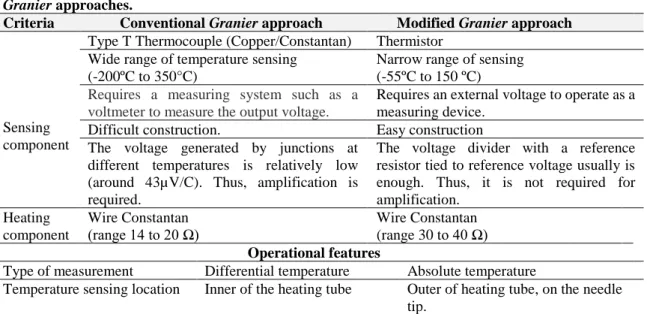
Fig.III. 2: The modified Granier sensor (mG) design. a) Building components: 1. Constantan wire; 2. Thermistor; 3. Thermistor terminals; 4. Hypodermic needle; 5. Stainless tube. b) Schematic structural difference between modified Granier sensors and conventional sensors. ... 29
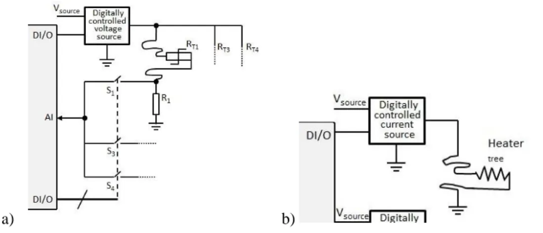
Fig.III. 3: Schematic connections of: a) the thermistors interface; b) the heater circuits. ... 30
Fig.III. 4: Construction diagram of the weighing device(mLy): 1. Load cell; 2. Superior plate (holding soil component); 3. Inferior plate (base supporting); 4. Power and communication data cable; 5. Height scale; 6. Hex Nut. ... 31
Fig.III. 5: Schematic of the amplifier used in the modified microlysimeter. R1, R2 are resistors. GND1 is the ground. DC (direct current). ... 32
Fig.III. 6: The transfer characteristic of the mLy obtained after performing a calibration procedure with an electronic scale. ... 33
Fig.III. 7: The transfer characteristics related to the soil mass ranging. ... 34
Fig.III. 8: The commercial Peltier cell image ... 35
Fig.III. 9: Schematic of the amplifier used in the Peltier cell interface. R1, R2 and R3 are resistors. GND1 is the ground. ... 35
Fig.III. 10: The schematic Arduino Mega 2560 used as the local controller. ... 36
Fig.III. 11: General view of the SOIS software organisation. ... 37
Fig.III. 12: The data control system organisation ... 37
Fig.III. 13: The SOIS data processing organisation ... 41
Fig.III. 14: Schematic illustration of computation: a) transpiration; b) soil evaporation and soil moisture; c) soil latent heat flux, soil heat flux and soil heat storage. ... 42
Fig.III. 15: Schematic flowchart of the FAUSY algorithm. ... 43
Fig.III. 16: Learning time (LT) and forecasting time (FT) temporal sequence ... 47
Fig.III. 17: Substrate-moisture characteristic curves for the studied substrates, respectively, S1, S2 and S3; θ – moisture content (cm3 cm-3). Gray marks: θ FC estimated for the respective substrates. ... 55
Fig.III. 18: The tipping bucket rain gauges at the Herbarium building of the University of Lisbon, Instituto Superior de Agronomia (ISA) ... 56
Fig.III. 19: Diagram of the sap thermal dynamic around the heater sensor (Theat) ... 58
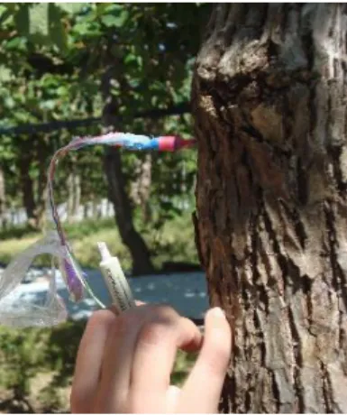
Fig.III. 20: Experiment in a greenhouse at the Instituto Nacional de Investigação Agrária e Veterinária (INIAV-Dois Portos): a) Potted olive tree with a Granier sensor, heater switched OFF; b) Potted olives trees with a Granier sensor, heater switched ON. ... 59
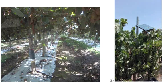
Fig.III. 21: Experimental field set up: a) kiwi orchard in Quinta das Picas, São Salvador de Briteiros; b) vineyard in Adega Carapateiro- EN118 Porto Alto – Alcochete. ... 61
Fig.III. 22: The installation of modified Granier sap flow sensors on Kiwi plants in Briteiros (Guimarães, Portugal). ... 62
Fig.III. 23: The installation of sap flow sensors on the vineyard -Adega Catapereiro: a) modified Granier sensor; b) Conventional Granier sensor. ... 62
xiv
Fig.III. 26: Instrumental eddy covariance measurements (EC) in Vineyard field experiment – Quinta do Marquês, Oeiras. a) EC localisation on the parcel. b) the sensors and the metal observation tower at the height of 2.5 m ... 66 Fig.III. 27: Vineyard scheme and location of the tower used for micrometeorological measurements. ... 67 Fig.III. 28: Schematic of the SOIS set up in the vineyard field experiment– Quinta do Marquês, Oeira ... 68 Fig.IV. 1: Visual analysis of the daily behaviour of natural temperature gradients and the accessible
explicative variables (normalised data) in the timeline, namely, reference evapotranspiration (ETo), solar radiation (Rs) and relative humidity (RH) over the interval of days: a) [100,110] and b)
[150,160]. ... 72 Fig.IV. 2: Comparing between the residual error obtained for the dependent variable NTG and the
explicative variable combinations: Rs(t) × RS(sbt2) × RH(t) × RH(sbt2) and ETo (t) × ETo (sbt2). .. 74 Fig.IV. 3: Comparison of transpiration estimates (F [mm d-1]) with the FAUSY algorithm (F_fausy [mm d
-1]), using the not adjusted procedure (F_not adjusted [mm d-1]) and the adjusted procedure
(F_adjusted [mm d-1]) and the respective linear regression curves for sensors: (a-b) sensor G7; (c-d) sensor G8; (e-f) sensor G5. ... 77 Fig.V. 1:The green roof lab-rooftop of the Herbarium building of the University of Lisbon, Instituto
Superior de Agronomia (ISA) (https://www.facebook.com/thegreenrooflab/?ref=bookmarks). ... 79 Fig.V. 2: Bias analysis (root mean square error (RMSE)) of the hourly mean volumetric substrate moisture
(θh[cm3cm-3]) for the treatments: T3, T5,T6,T8 and T11 with mLy and TDR data clustered on an hourly basis. ... 81 Fig.V. 3: Bias analysis (root mean square error (RMSE)) with mLy and TDR data. Left vertical axis: hourly mean volumetric substrate moisture scaled to a daily basis (θd [cm3cm-3]) for the treatments: T3, T5, T6, T8 and T11. Right vertical axis: reference evapotranspiration estimates (ETo [mm d-1]). ... 82 Fig.V. 4: Circadian curve analysis from the day 220 to day 232 for the treatments: a) T3; b) T5; c) T6; d)
T8; e) T11. Left vertical axis: hourly mean volumetric substrate moisture content (θh [cm3 cm-3]) measured with mLy (full line) and TDR (dash line) sensors. Right vertical axis: irrigation depths: a) I60 [mm d-1] (60%ETo); b) I60 [mm d-1] (60%ETo); c) I60 [mm d-1] (60%ETo); d) I100 [mm d-1] (100%ETo); e) I100 [mm d-1] (100%ETo). Reference evapotranspiration (ETo [mm d-1]). ... 83 Fig.V. 5: The hourly mean volumetric substrate moisture content θh [cm3cm-3] from day 221 to day 225,
with the weighing device data (mLy11) and the reflectometer sensor data (TDR11). Irrigation event (Blue Dash line); Spent time to water redistribution (red line); Maximum values measured with mLy11 (green arrows) ... 84 Fig.V. 6: Linear regression between diary evapotranspiration estimates (ET [mm d-1]) and reference
evapotranspiration (ETo [mm d-1]) observed with mLy devices (mLy) and reflectometer sensors (TDR) on treatments: a) T3; b) T5; c) T6; d) T8; e) T11. ETo estimates (red dash line), TDR estimates (black dash line), mLy estimates (black line). ... 86 Fig.VI. 1: Comparative offset between conventional and Biot approaches. a) offset between TMAX(Conv) and
TMAX(Biot) obtained with the sensor Theat(P01); b) offset between TMAX(Conv) and TMAX(Biot) obtained with the sensor Theat(P02); c) offset between Tno_heat and T∞ obtained with the sensor Tno_heat(P01); d) offset between Tno_heat and T∞ obtained with the sensor Tno_heat(P02). ... 90
xv
Fig.VI. 2: Comparative diagram between the sap flux density computed from the Biot approach (uBiot [m3 m-2 s-1]) and computed from the conventional Granier approach (u
Conv [ m3 m-2 s-1]) in comparison to the sap flux density observed for gravimetric test (uGrav [ m3 m-2 s-1]) on the sensor: a) P01, circadian curves (days 85 and 86 (2018)); b) P01, regression curve uGrav versus uBiot and uConv; c) P02, circadian curves (days 86 and 87(2018)); b) P02 regression curve uGrav versus uBiot and uConv. ... 92 Fig.VI. 3: Observations of the temperature differences decrease (∆T [ºC]), ranging from 3.16 to 3.09 ºC
before to up to higher values ranging from 3.09 to 3.28 ºC... 92 Fig.VI. 4: Comparative diagram between the sap flux density computed from the conventional Granier
approach (uConv [m3m-3s-1]) in comparison to the sap flux density observed for gravimetric test (uGrav [m3m-3s-1]) on the sensor: a) C01, circadian curves (days 107-108 (2018)); b) C01, regression curve uGrav versus uConv; c) C02, circadian curves (108-110 (2018)); b) C02 regression curve uGrav versus uConv. ... 93 Fig.VI. 5: Comparative diagram between the Granier sap flow indexes with the sensors (P01, P02, C01 and C02) from day 86 to day 102. ... 94 Fig.VI. 6: Comparative diagram between the sap flow measured in potted olive tree (P01) and computed for
Biot approach (Fbiot(P01) [mm h-1]), and the sap flow observed for gravimetric test (Fgrav(C01) [ mm h-1]) in potted olive tree (C01) and computed for conventional Granier approach (Fconv(C01) [ mm h-1]) in the days 107 and 108. ... 95 Fig.VI. 7: Comparison of the hourly mean air vapour pressure deficit (VPD [kPa]) from data collected at
INIAV-Dois Portos meteorological station (days 86 to 108 (2018)) with: a) sap flow from modified
Granier sensors (FbiotP01 [mm h-1]); b) sap flow from the conventional Granier sensor (Fconv(C01) [mm h-1]); c) Comparison between Fbiot
(P01), Fconv(C01) and VPD estimates. ... 96 Fig.VI. 8: a) Evolution of the temperatures provided by two tree sensors; b) Distribution of the relative
error obtained when measuring the same temperature with the heater sensors (Theat[ºC]) and referential sensor (Tno_heat [ºC]). ... 98 Fig.VI. 9: Distribution of the relative error obtained when measuring the same temperature with heater
sensors (Theat[ºC]) and referential sensors (Tno_heat [ºC]). ... 98 Fig.VI. 10: The heater sensors (G2Jheat[ºC]) and referential sensor (G2Jno_heat [ºC]) inserted into a tube filled with cork ... 99 Fig.VI. 11: Evolution of the power applied to the modified Granier sensor and temperatures measured with the two tree sensors (G2Jheat[ºC] and referential sensor G2Jno_heat [ºC]). ... 99 Fig.VI. 12: Differential temperature measurements for sap flow estimation before (∆T (dash line)) and after (∆Tadj (full line) offset correction: a) G5J sensors, b) G6J sensors. ... 100 Fig.VI. 13: The temperature differences (ΔT [ºC]) collected from the sap flow sensors in the Adega
Catapereiro Vineyard from day 232 to day 240 (2017). The hourly mean (ΔTh [ºC]) with mGSP02 and CGr3 sensors were clustered on an hourly basis (Hour/24). Full square - modified Granier data (ΔTh (mGSP02)). Empty square - conventional Granier data (ΔTh (CGr3)). ... 102 Fig.VII. 1: a) Soil moisture (θh [cm3 cm-3]) related to the Granier sap flow index k
Conv observed on single lemon tree experiment from day 133 to day 135 (2016); b) Linear regression to model the relationship between Granier sap flow index (kConv) and soil moisture (θh [cm3 cm-3]). ... 105 Fig.VII. 2: The Granier sap flow index curve and the soil heat flux curves at two depths: G0, G15 observed
xvi
Nova Oeiras1. ... 107 Fig.VII. 4: Footprint analysis of eddy covariance data: a) footprint prediction; Qf [m-1] - footprint function;
x [m] – horizontal distance between the measuring point and a point on the region of origin of the
flows; b) Cumulative footprint prediction; Qc – Cumulative normalised flux; xL [m] – distance between the measuring point and the boundary of the source region of the fluxes. ... 108 Fig.VII. 5: Sensible heat flux (HEC [W m-2]) and latent heat flux (LEEC [W m-2]) recorded by eddy
covariance methodology in discontinuous time on the days 271 to 294 ... 110 Fig.VII. 6: Hourly mean values obtained from eddy covariance measurements (EC) clustered on an hourly
basis. a) evapotranspiration (ETEC [mm h-1]); b) latent heat flux (LEEC, W m-2) and sensible heat flux (HEC, W m-2). ... 110 Fig.VII. 7: Comparative diagram of raw data obtained between the days 288 and 290 with an eddy
covariance instrument (EC) and a modified Granier sensor (SP32L): a) circadian curve of the evapotranspiration measurements (ETactual(EC) [ mm h-1]) and the adjusted sap flow rate measured in function of conventional Granier sap flow index (kConv_Adj) and Biot number Granier sap flow index (kBiot_Adj) approaches; b) dispersion of the transpiration data (F(kBiot)adj and F(kConv)adj) around the fitted line of the ETactual(EC)... 112 Fig.VII. 8: Comparison of the circadian curve from day 288 to day 290 (2016) between soil moisture
estimated with the mLy4 (θmLy4 [cm3cm-3] – empty circle - right vertical axis) sensor and the transpiration (F [mm h-1] – left vertical axis) estimates based on the sap flow approaches: conventional Granier sap flow index (kConv) (dash line) and Biot number Granier sap flow index (kBiot)(full line)... 113 Fig.VII. 9: Comparison of the circadian curve from day 288 to day 290 (2016) between soil moisture
estimated with the mLy4 sensor (θmLy4 [cm3cm-3] (empty circle - right vertical axis) and soil heat storage measured with the pair of Peltier cells (ΔGPcell4 [W m-2] (full circle – left vertical axis). ... 114 Fig.VII. 10: Comparative linear regression between the soil heat storage measured with the pair of Peltier
cells (ΔGPcell4 [W m-2]) and the volumetric soil moisture estimated with the weighing device (θmLy4 [cm3 cm-3]). The data were collected between the day 253 to day 290 (2016). ... 114 Fig.VII. 11: Comparison of the circadian curves for the soil heat storage measured with the pair of Peltier
cells (ΔGPcell4 [W m-2] empty circle - right vertical axis) and the sap flow rate measurement (F [mm h -1] - left vertical axis) with the modified Granier sensor (SP32L) in function of conventional Granier sap flow index (kConv) ( dash line) and Biot Granier sap flow index (kBiot) (full line). ... 115 Fig.VII. 12: Comparative linear regression between the soil heat flux near the soil surface (G0 [W m-2]) and the soil heat flux at 10 cm depth (G10 [W m-2]) measured with the pair of Peltier cells. The data were collected between the day 287 to day 296 (2016). ... 115
xvii
LIST OF TABLES
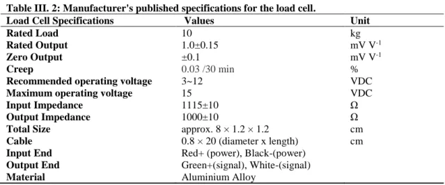
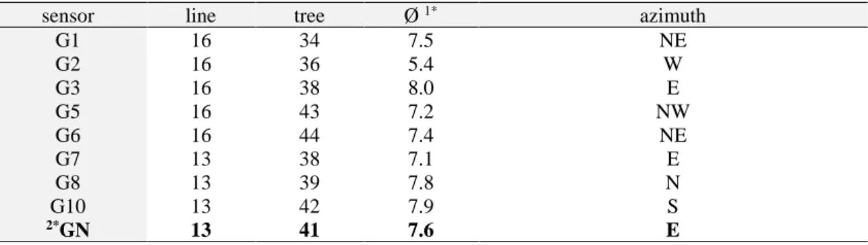
Table III. 1: Technical comparison between the original Granier sap flow and the modified Granier approaches. ... 28 Table III. 2: Manufacturer's published specifications for the load cell. ... 32 Table III. 3: Summary of the experimental sites ... 49 Table III. 4: Description of the sensors in the olive trees. 1*: Trunk diameter to height h (30 cm); 2*: heater
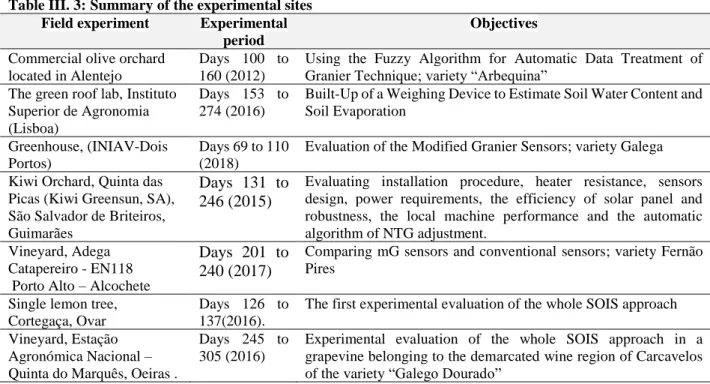
switched off. ... 50 Table III. 5: ΔTMAXna [ºC] and ΔTMAXadj [ºC] obtained from measurements in the 10 initial days
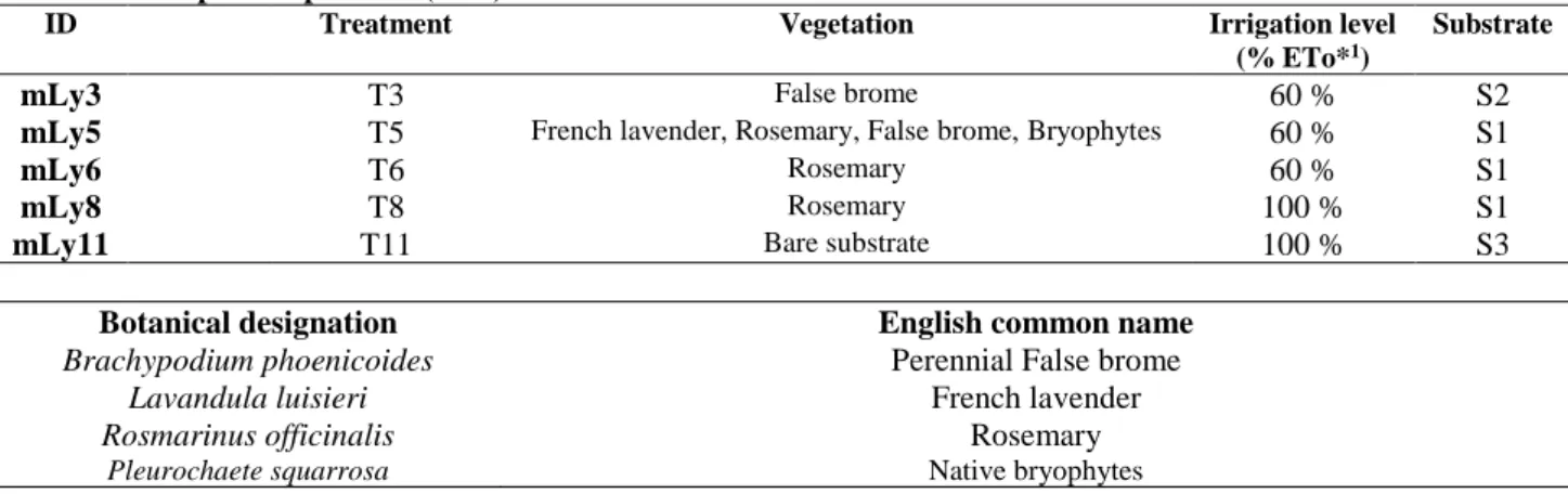
(DOY[100;110]) ... 51 Table III. 6: Experimental set up in trays with three different substrates, submitted to two irrigation levels
and the botanical Latin designations of the plants used. *1: Irrigation level based on 60 % (I 60) and 100% (I100) of the reference evapotranspiration (ETo) ... 53 Table III. 7: Characteristics of the substrates used in the experimental sets (OM – organic matter, θFC – field
capacity, θWP – wilting point, ρb – bulk density, Ksat – saturated hydraulic conductivity). *1: not classified given the high OM content ... 53 Table III. 8: Experimental set up in trays with mLy devices and TDR sensors. *1: Effective depth of the
mLy plate (zmLy); *2: Effective depth of the TDR sensors (zTDR); *3: Horizontal distance between the mLy devices and TDR sensors; *4: Irrigation level based on 60 % (I
60) and 100% (I100) of the
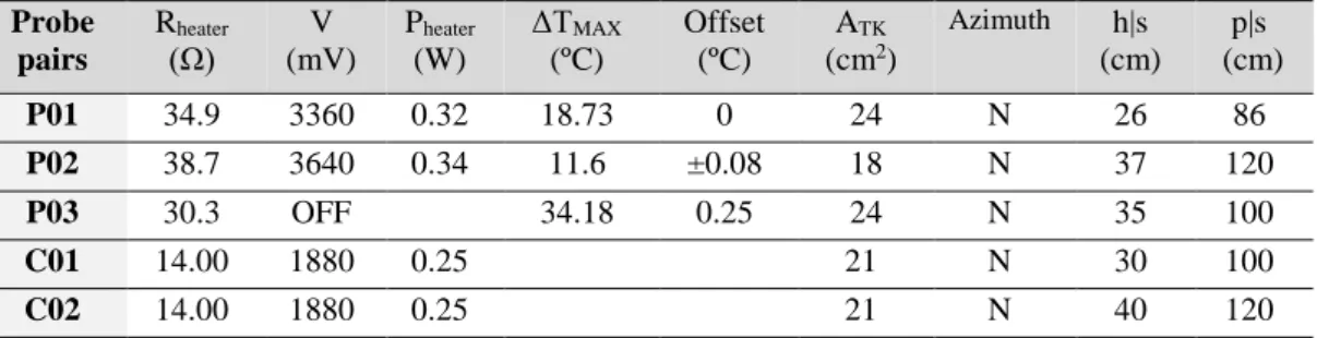
reference evapotranspiration (ETo) ... 54 Table III. 9: Description of the resistances of Theat, sensors dimensions, the heat maxima reached in a
confined environment, diameter trunk and sensor localisation on the tree.Rheater: Nominal Resistance of the heater; V: Voltage applied on resistance; Pheater: Nominal power resistance; ΔTMAX: Maximum temperature difference; ATK: Trunk area; h|s: distance between Theat and soil surface; p|s:height of the tree from top to soil surface. ... 60 Table III. 10: Characteristics of sensors used on kiwi orchard trial.Rheater: Nominal Resistance of the heater; I: Nominal electrical current; ATK: Area of the trunk ... 61 Table III. 11: Characteristics of sensors used on the vineyard – Adega Catapereiro.Rheater: Nominal
Resistance of the heater; h|s: Distance between Theat and soil surface; ATK: Area of the trunk ... 63 Table III. 12: Physical characterisation of soil in the vineyard field experiment – Quinta do Marquês,
Oeiras. ... 65 Table III.13: Specifications of modified Granier sensors and weighing devices installed in the vineyard
field experiment -Quinta do Marquês, Oeiras ... 69 Table IV 1: Mean squared error (MSE) of the four variable combinations during the DOY interval [100,
110] (learning time). ... 73 Table IV 2: Performance of FAUSY algorithm computed by residual error equations (4-6) computed from
mean transpiration [mm d-1] ... 74 Table V. 1: Bias analysis using root mean square error (RMSE) as a statistical indicator for comparison of
the global mean volumetric substrate moisture (θ [cm3cm-3]) between mLy devices (mLy) and Reflectometer sensor (TDR) ... 80
xviii
xix
LIST OF ABBREVIATIONS AND SYMBOLS
Symbol description
θ̅ Global mean mass moisture [cm3 cm-3] ∆θ Change of substrate water content [cm3 cm-3]
aj, bj and cj Parameters of the triangular membership function for the jth fuzzy set. Amly Area of the superior plate of the weighing device [cm2]
ATK Area of the conducting xylem section [cm2] Biot Biot number
CV Coefficient of variation [%]
Cv Soil volumetric heat capacity [J m-3 ºC-1 ] D Deep percolation observed [mm]
d Height displacement of reference plane [m] DOY Day of Year
DZ Depletion depth [mm] E Evaporation [m s-1]
e Event.
Es Soil evaporation rate [mm h-1]
EsmLy Soil evaporative rate from weighing device [mm h-1] ET Evapotranspiration rate [mm h-1]
ETc Crop Evapotranspiration [mm d-1]
ETEC Evapotranspiration rate from Eddy Covariance [mm h-1] ETo Reference evapotranspiration [mm h-1] and [mm d-1]. F Sap flow rate [m3 s-1]
Fadj Sap flow rate adjusted [m3 s-1] FAUSY Fuzzy Algorithm Automation System
FBiot(mG) Sap flow rate (modified Granier sensors (Biot approach)) [m3 s-1] and [mm h-1] FConv(CO) Sap flow rate from conventional Granier sensors [m3 s-1] and [mm h-1]
FConv(mG) Sap flow rate (modified Granier sensors (conventional approach))[m3 s-1] and [mm h-1] FGY Sap flow rate from gravimetry approach [m3 s-1] and [mm h-1] and [mm h-1]
fmLy Calibration factor of weighing device [mV g-1] Fna Sap flow rate not adjusted [m3 s-1]
Fpred Sap flow rate predicted [m3 s-1] FSj Fuzzy set jth.
FV Explicative fuzzy variables. fΔj Triangular membership function. Gconv Conventional Granier sensor GM Granier heat dissipation method
xx
I100 Daily irrigation depth 100% ETo [mm] I60 Daily irrigation depth 60% ETo [mm] k Thermal conductivity [W m-1 ºC-1]
kadj Adjusted Granier sap flow index (Granier coefficient). kBiot Adjusted Granier sap flow index in analogy at Biot number
kConv Granier sap flow index (original approach)
kGadj Adjusted Granier flow index (FAUSY approach) kGna Not adjusted Granier sap flow index (FAUSY approach) kGpred Predicted Granier sap flow index (FAUSY approach) L Latent heat of vaporization and [J m-3]
LE Latent heat flux [W m-2]
LE– Latent heat of vaporization [W m-2] LE+ Latent heat of condensation [W m-2] LEsoil Soil latent heat flux [W m-2] lrc Linear regression curve m a.s.l Metres above sea level [m] mG Modified Granier sensor mLy Weighing device MSE Mean square error nfr Number of fuzzy regions. NTG Natural temperature gradient [℃]
NTGobs(t) Observed temperature difference by the Granier sensors switched OFF at t time [ºC] NTGpred(t) Predicted NTG via FAUSY at t time [℃].
P Precipitation [mm] Pcell Calibrated Peltier cell
PFC Percentage of FAUSY contribution [%]
Pheater Nominal power resistance of heater element [W] Qc Cumulative normalised flux
Qf One-dimensional footprint (or footprint function) [m-1] RE Residual error.
REf Residual error from FAUSY [m3 s-1]
REna Residual error from manual computation [m3 s-1] REpred Residual error of sap flow predicted. [m3 s-1] RH Relative humidity [%]
RMSE Root mean square error Rs Solar radiation [W m-2] S Soil heat storage [W m-2]
S∆t Variation of soil heat storage per time t on ∆z soil layer [W m-2] SBT Steps backwards over time
xxi
SOIS Smart Orchard Irrigation System SOS SOIS software
stmLy Signal of mLy device in t time [mV] t Variable time [s]
T no_heat Reference temperature [Cº]
T Temperature [ºC] TDR Reflectometer sensor
Theat Temperature heater sensor [Cº]
Time Fraction of day (1/48, 12/48, …, 48/48)) variable TMAX Maxima temperature reached [Cº]
TSOIL Soil temperature [Cº] u Sap flux density [m3 m-2 s-1]
uadj Adjusted sap flux density. [m3 m-2 s-1]
uBiot Adjusted Granier sap flux density [m3 m-2 s-1] (Biot number approach)
uConv Granier sap flux density [m3 m-2 s-1] (conventional approach)
UD Universe of discourse.
una Not adjusted sap flux density [m3 m-2 s-1] upred Predicted sap flux density [m3 m-2 s-1] Vd Relative output to each event e VPD Vapour pressure deficit [kPa] Wi Actual mass balanced in i time[g] WMAX Maximum mass value weighted WMIN Minimum mass value weighted
WSB Weighed soil boundary
x Actual value of a variable.
xL Distance between the measuring point and the source region of the fluxes [m] xmax Maximum normalised value of a variable.
xmin Minimum normalised value of a variable. xn Normalized value of a variable.
z Subscript representative of the soil depth zmLy Depth between the mLy plate and surface [cm] zo Aerodynamic surface roughness[m]
ΔT Temperature difference [ºC]
ΔT(t) Temperature difference at t time [ºC] ΔTadj(t) ΔT adjusted by NTG observed at t time [ºC] ΔTMAX Maximum temperature difference [ºC]
ΔTMAXadj Adjusted maximum temperature difference [ºC] ΔTMAXna Not adjusted maximum temperature difference [ºC] ΔTna(t) Not adjusted temperature difference at t time [ºC]. ΔTpred(t) Predicted temperature difference at t time [ºC]. θ Actual mass moisture [cm3 cm-3]
xxii
2
CHAPTER 1
I. CHAPTER 1: Introduction
I.1. General framework
The efficient use of water in agriculture is at the forefront position of the issues related to the sustainable exploration of hydric resources. Water scarcity arises not only in arid and drought-prone areas but also in regions where rainfall is abundant. According to Pereira et al. (2002), water scarcity concerns the quantity and the quality of the available water. For this reason, several studies point out solutions to cope with insufficiency of agricultural water demand, investigating the ability to improve quality and use a minor quantity of water without producing new environmental impact and reduction of the crop productivity (Pereira et al., 2009; Dias et al., 2010).
The scientific community has been impelled to develop new technologies for the efficient use of water based on the accurate information of crop water requirements at different growth cycles and soil water hold capacity (Pereira et al., 2012). In the face of the apparent performing complexity to determine the crop water requirements, a range of decision-making tools for irrigation schedules have been developed aiming at optimising the water use while maintaining enough levels of crop productivity.
The central challenge for irrigation scheduling based on the crop water requirements and soil characteristics involves the development of specific methodologies for ranges of yield, environments and soil. Unfortunately, the increased sophistication, operationality and easy-maintenance of the devices, have not necessarily improved the accuracy of data collection. In fact, it has facilitated the carry out of measurements by individuals having insufficient experience, care, or understanding of the physics and methodology, resulting in data showing relatively reduced accuracy (Jensen & Allen, 2016). Also, Allen et al. (2011a) have summarised common errors to modern crop water requirements methodologies.
INTRODUCTION CHAPTER 1
3 Several reasons explain the failure of these approaches, e.g., economic aspects, problematic maintenance, non-existent training and deficient interaction among all agents involved, i.e., researchers, technicians, farmers and governmental agencies (Smith et al., 1996; Blazy et al., 2009; Grové, 2011). Consequently, research and demonstration efforts are sometimes wasted. The challenge to researchers concerns developing a technological alternative for the efficient use of water that is readily adaptable to agricultural environment categorised for the economic, social and technical constraints.
The development of innovative technology for applications in the agricultural environment should take low cost, easy maintenance, and life-long training of the users as mandatory requirements. Also, it should consider the robustness and easy-handling of all devices installed in the field. Finally, it is justifiable to reflect on the interactive communication between researchers, technicians and farmers. A low-cost open system attends to these requests, since providing unrestricted and transparent access to hardware and software designs. It takes advantage of new technologies associated with efficient mathematical tools, which permits building, replicating, modifying or repairing transducers at low cost and streamlining aid of experts or professionals.
The Smart Orchard Irrigation System (SOIS), defined as a low-cost open system, proposed here allows improving the transferability and applicability of the irrigation scheduling techniques based on specific crop water requirements and soil characteristics. In this context, this work addresses the design and implementation of SOIS as a means to manage the watering in orchards and vineyards, demonstrating their adaptability, advantages and challenges.
I.2. Objectives
The general objective of this thesis is to design and to implement the low-cost open, interactive and user-friendly system for orchards and vineyards irrigation management to improve irrigation scheduling, aiming at the efficient use of water in agriculture.
The specifics objectives are:
a) Design the low-cost open system characterised by resorting to easy-to-use and inexpensive materials and methods;
b) Develop a fuzzy logic algorithm for the automatic data analysis of the data originated from the low-cost open system.
4
c) Optimize the Granier sap flow sensors by using thermistors as the temperature sensing components, which will allow improving the computation of the Granier equation parameters;
d) Develop and manufacture the material and methods for a novel automatic microlysimeter that is characterised by being deprived of a container, aiming to measure the under-canopy in continuo;
e) Use Peltier cells as an alternative soil heat flux sensor, aiming to measure the soil heat flux in two soil depth and estimating the soil latent heat flux.
I.3. Original Contributions
a) A new system to control the use of water in commercial orchard and vineyard was developed resorting to low-cost hardware and software parts.
b) A fuzzy logic algorithm automation system (FAUSY) for automatic and in real time sap flow data analysis was established and validated.
c) A modified Granier sap flow sensor was advanced and validated using thermistors, obtaining success in adopting a new approach to compute the Granier sap flow index.
d) A novel automatable weighing device was developed to measure the under-canopy soil evaporation measurement, which can be used in continuous time.
e) A Peltier cells based methodology was proposed and tested, which estimates the soil latent heat flux from the story.
I.4. Outline of the thesis
This thesis is organised into eight chapters. Chapter I describes the problem reading, the objectives required to solve the problem and the framework of the thesis.
The State of the Art is overviewed in Chapter II. In this chapter, the first and second sections address the solutions that have been proposed in the scientific literature for the efficient use of water in orchards and vineyards. The usual procedures for the crop evapotranspiration, soil evaporation and transpiration sensing are also described. The second section ends with an overview on the current literature concerning the ET modelling for orchards and vineyards. Finally, the last topic presents the concept of the low-cost open system applied to ET measurement.
INTRODUCTION CHAPTER 1
5 Chapter III describes the concept, material and approaches concerning the Smart Soil Irrigation System (SOIS). Firstly, in sequence are described the SOIS concept, its architecture, and the inputs and outputs required for integrating the two components of the evapotranspiration and the physical principles with which the SOIS is constructed, i.e., transpiration and soil evaporation estimates. Also, Chapter III describes the material and methods adopted for the assembly, manufacture and trial implementation, as well, refers to the implemented mathematical tool.
The following chapters IV, V, VI and VII describe the experimental working using partial and global SOIS approach. Finally, chapter VIII highlights the main conclusions and future perspectives.
6
STATE OF ART CHAPTER 2
7
CHAPTER 2
II. CHAPTER 2: Crop Evapotranspiration and Efficient Water Use in Orchards and Vineyards
The adequate use of water for irrigation figure weights different water balance components, the relationships between these components and takes into account losses during storage, conveyance and application to irrigation plots (Hamdy, 2007). Also, it involves a broad assortment of disciplines, e.g., agronomy, plant physiology and engineering (Nair et al., 2013), including mixed approaches for the rational and sustainable use of water in agriculture, for example, water productivity and water efficiency. As defined by Pereira et al. (2002), the term “water use efficiency” should be used to measure the water performance of plants and crops, irrigated or non-irrigated, to produce assimilates, biomass and harvestable yield. While the term “water productivity” should be adopted to express the quantity of product or service generated by a given amount of water used. In the sense of taking a broad view of the water consumption with efficient and productive strategies, the crop evapotranspiration information is an essential term in that equation (Pereira, 2007). Thus, the crop evapotranspiration sensing and modelling are prerequisites for efficient and productive water use.
Allen et al. (1998, 2007b) describe the term evapotranspiration (ET) as a combined process, whereby liquid water is transformed to water vapour and removed from the evaporating surface and contained in plant tissues to the atmosphere. Also, ET is driven by atmospheric demand as well as soil water potential and hydraulic conductivity. However, unlike soil evaporation, plant transpiration is regulated by opening and closing of the stomata (Kool et al., 2014). Thus, ET should be computed and monitored by evaluation of the biophysical parameters and variables related to the hydric and heat transference inside of the vadose zone, among plants, soil and atmosphere (Allen & Pereira, 2009; Paço et al., 2012).
The orchards and vineyards, named as sparse canopies, can be described as surface types which are partially covered with plants, permitting a significant part of the available radiative energy heating the bare soil (Hurk, 1996). According to sparse canopies, the sensing and modelling of the transpiration (T) and soil evaporation (Es) in two independent components, i.e., ET partitioning, can be useful for assessing water use efficiency (Kool et al., 2016). Mainly, it can incorporate the effects of the different canopies and soil characteristics in the discrete
8 estimation of T and Es (Odhiambo & Irmak, 2011), permitting to use different combinations, depending on the scale of interest, cover type, study objectives, and available resources (Kool et al., 2014).
II.1. ET partitioning sensing for orchards and vineyards
The crop evapotranspiration sensing in ET partitioning approach requires the employment of sensors and techniques, with which both components, transpiration (T) and soil evaporation (Es) are measured separately, or the ET component is measured, and one of the elements (T or Es) is taken as the residual of the other two.
The methods discussed in this thesis are those that recurrently are used in commercial orchards and vineyards aiming to estimate the sap flow rate into the tree trunk and under-canopy soil evaporation. Relevant scientific works include typically, the use of sap flow sensors and microlysimeter devices for transpiration and soil evaporation estimates, respectively. Also, the eddy covariance technic among others, due to being mostly used in global ET sensing for research purposes.
II.1.1. Transpiration sensing
The direct measurement of crop transpiration under field conditions can be done using several methods that include, e.g., stem flow gauges, weighing lysimeters and environmental chambers that cover a volume (>1 m3) of plants (Lascano et al., 2016). However, the most
techniques designed to T estimations for orchards and vineyard install sensors in the trunk using heat as a sap motion tracer because the stem is limited by a single route of water extraction along the soil-plant-atmosphere continuum (Fuchs et al., 2017). Fernández et al.(2017) summarised this approach in heat balance, heat pulse and constant heater methods, which are fundamentally different in their operating principles (Smith & Allen, 1996; Vandegehuchte & Steppe, 2013), e.g., the localisation of sensors in relation to the conductive organ, the methods to the calculation of the sap flow, the size of the stems and the frequency of measurement. Also, their potential for irrigation scheduling has been assessed (Fernández, 2017), which are chosen to be robust and reliable enough for operation in the field over extended periods, automatable and implemented with low cost and easy-to-use data transmission systems (Smith & Allen, 1996). Thus, these sap flow sensors have many applications conferring a high potential for the efficient use of water in orchards and vineyards (Fernández, 2014).
STATE OF ART CHAPTER 2
9 Currently, two commercially available focal methods are employed to sap flow quantification (Fernández et al., 2017) that are appropriated to use in orchards and vineyards (Kool et al., 2014), respectively, the Granier heat dissipation method (Granier, 1985, 1987) and the heat pulse-sap velocity method (Green et al., 2003). Given the ordinary replication and automation of these sap flow approaches, they have been widely used on main woody stems to quantify the tree transpiration (Granier et al., 1996).
The well-known Granier heat dissipation method (GM) (Granier, 1985, 1987) is the most widely applied sap-flux density method because of its simplicity and low cost (Vandegehuchte & Steppe, 2013). It consists of constant heater methods, which are used to quantify sap flow velocity based on temperature dissipation from a constant heating source into the stem. It requires one or more pairs of heated and unheated sensors that are inserted radially into the sapwood. Sap velocity is determined from the temperature differences, using an empirical flow index and equation that is subsequently calibrated to plant size using sapwood area. That equation assumes that the maximum temperature difference corresponds to zero flow conditions and the unheated sensor is the intangible referential temperature.
The heat pulse-sap velocity method (HM) relies on short heat pulses applied into the conducting sapwood layer, being the mass flow of sap is determined from the velocity of the heat pulses moving along the stem (Green et al., 2003). It allows the quantification of sap flow velocity based on temperature response curves to a short heat pulse into the stem, where time delay for temperature rise is assumed to be proportional to sap flow velocity.
The similarities between Granier heat dissipation method and heat pulse-sap velocity method stand out in that both methods:
i) use a part of the conductive organ as a sampling of the whole tree; ii) are invasive methods, since the sensors are located within the sapwood;
iii) use medium to large steam diameters (i.e., > 30 mm) (Smith & Allen, 1996);
iv) require that the area of conductive tissue must be estimated accurately; v) can be implemented with automatable and inexpensive technology;
In contrast, the differences when comparing GM and HM approaches are the physical principles of HM in opposition to the GM empirical approach, and the required installation precision of the HM sensors into the tree.
HM is derived from thermodynamic principles, which require elaborate and understanding computation. Thus, it is supposed not to require calibration. On the other hand, the original empirical Granier equation cannot be used for GM sensors with deviating design (Lu et al., 2004;
10 Fuchs et al., 2017) since that any modification of methodology needs recalibration. However, GM approach computation is simple and easily interpreted.
The GM methodology uses sensors separated with a distance free of accuracy (Vandegehuchte & Steppe, 2013), of around 10 cm. Contrarily, HM sensors must be installed in exact measure, since the sensors misalignment can lead to significant errors. HM calculations are highly sensitive to the distance between the heater and the sensors, which can lead to either an over or underestimation of transpiration. Also, the reverse flow and low or very high flux densities cannot be measured because a temperature equilibrium between upstream and downstream sensors does not establish under those conditions. It performs poorly at low flow rates and has unresolved limitations under conditions of high flows (Vandegehuchte et al., 2015; Miner et al., 2017). It suggests that the HM methods have high precision but a bias towards correct plant water use and must be calibrated (Forster, 2017).
A significant limitation that applies to all heat pulse and constant heater methods is found in scaling from sap flow to whole plant T, where individual trees introduce uncertainty due to variation in exposure to solar radiation and aerodynamic turbulence (Kume et al., 2010). Also, the relationships and calibrations may change with soil moisture, LAI, disease (Allen et al., 2011). To conclude, the implanting sensors can cause mechanical damage and interrupt flow by occlusion or blocking of the plant’s vascular tissues and the area of conductive tissue must be estimated accurately. Clearwater et al. (1999) showed that sap velocity could be severely underestimated if portions of the heated sensor are in contact with inactive xylem or bark.
The Granier heat dissipation method has been widely used for larger stems and has been reported to give moderate to reasonable results. For example, olives (Cammalleri et al., 2013; Paço et al., 2014b), Mediterranean evergreen oak savannah (Paço et al., 2009), date palms trees (Sperling et al., 2012), cherries orchards (Li et al., 2010), peach orchards (Paço et al., 2012),vineyards (Fernández et al., 2008; Ferreira et al., 2012). However, some restrictions were observed in using the GM approach. Wilson et al. (2001) observed errors associated with scaling single tree estimates and measurement errors associated with ring-porous water conducting elements. Ferreira et al. (2008) observed an underestimation of T with GM data when compared to data from eddy covariance (EC) micrometeorological method. Bush et al. (2010) suggested that the original Granier calibration should not be assumed for all cases. Masmoudi et al. (2011) observed that sap flow estimates within young olive trees varied with the sensor position.
In conclusion, weighting the pros and cons, the principal advantages of the GM method as an alternative to others sap flow sensors approach, appears to be the unproblematic installation, low-cost and low requirements for processing and interpreting the collected data (Fernández, 2014). It suggests that the upgrading of Granier methods should be a benefit, making the reliable
STATE OF ART CHAPTER 2
11 and robust sensors, capable of working under field conditions for the whole irrigation season, thus, being a useful tool for monitoring the water use in commercial orchards and vineyards.
II.1.2. Soil evaporation sensing
The importance of measuring soil evaporation (Es) lies in evaluating the effects of Es in the global ET. Es is coupling heat and water transfer between ground and atmosphere (Heitman et al., 2008c), which can be quantified based on the soil water and soil energy balance approaches. In this work context, i.e., for orchards and vineyards, it will be lined up the Es sensing methods that are suitable to estimate under-canopy Es, characterised for to vary spatially, depending primarily on soil water distribution, canopy shading, and under-canopy wind patterns (Kustas, 2014). In the soil water balance approach, the under-canopy Es sensing can be determined directly (e.g., microlysimeter) or indirectly resorting to sensors that measure the soil water content, computing the water changes in the timeline. Alternatively, Es estimates can resort to the soil energy balance approach for the soil sensible heat measurement along of the soil profile (Gardner & Hanks, 1966).
The microlysimeter based methodology is used to measure the Es, which provides a direct reference for under-canopy Es on the condition that the soil and the heat balance are similar to those in the surrounding area (Lascano & van Bavel, 1986; Plauborg, 1995) and it enables measurements of partial canopy cover conditions due to easy replication in different spatial soil water distribution, canopy shading, and under-canopy wind patterns (Kustas, 2014). Walker (1983) was one of the first to use microlysimeter for under canopy Es measurements. Since then, it has been widely used to measure evaporation from the soil surface of irrigated crops due to the accuracy of measurement and installation low-cost (Parisi et al., 2009).
Daamen et al. (1993) reviewed various microlysimeter designs, which ranged from 51 to 214 mm in diameter and 100 to 200 mm in depth and used in field studies for 1 to 10 days. However, the microlysimeters commonly reported in the literature, followed the original design by Boast & Robertson (1982), being typically in diameter as 8 –10 cm and depth range of 7–10 cm (Boast & Robertson, 1982; Evett et al., 2009) and experienced for different materials and sizes (Evett et al., 1995; Todd et al., 2000). Boast & Robertson (1982) pointed out that the microlysimeter gives accurate Es measurements provided the soil cores be replaced at least every 24–48 h to minimise discrepancies with field conditions. Also, it can be considered with reasonable accuracy when reaches to measurements better than 0.1 mm per hour evapotranspiration (Aboukhaled et al., 1982).
12 Kustas (2014) describes the typical methodology of microlysimeters as a representative vertical section of an undisturbed soil profile, which is inserted into a small cylinder open at the top. The microlysimeter is inserted back into the soil, aligning its upper edge level with the soil surface and weighed either periodically or continuously. The changes observed in weight reflect an evaporative flux. Due to practical implementation, the microlysimeters has been used widely for Es studies in orchards and vineyards, for example, coffee (Flumignan et al., 2011), cherry orchards (Li et al., 2010), olive orchards (Rousseaux et al., 2009; Paço et al., 2014b), peach orchards (Paço et al., 2012), vineyards (Heilman et al., 1994; Trambouze et al., 1998; Yunusa et al., 2004; Zhang et al., 2011; Ferreira et al., 2012; Poblete-Echeverría et al., 2012).
The microlysimeters are appreciated for simplicity and economy (Lascano & van Bavel, 1986), but are also considered time-consuming and constraints in time resolution as a result of manual weighing (Trambouze et al., 1998), limited representation of field conditions due to small sample size (Daamen & Simmonds, 1996) and the inability to measure during irrigation or rain (Flumignan et al., 2012).
The labour-intensive weighing issue has been resolved by placing the microlysimeter on a continuously weighing device (Daamen et al., 1993). Analysis of the costs for the mini-lysimeter system indicates that Es can be measured economically at a reasonable accuracy and sufficient resolution with a robust method of load-cell calibration (Misra et al., 2011), also, resorting to the multiplication of microlysimeters as much as necessary. Grimmond et al. (1992) experienced a portable and automatable mini-lysimeters (< 0.2 m2), which was compared with evaporative flux
measurements obtained using eddy correlation instrumentation. The results showed that the evaporative flux and soil moisture from the mini-lysimeters compared favourably with measurements that are representative of their surroundings. However, the microlysimeters compute the water loss by evaporation in the continuo, being always reset in irrigation or rain events. Unfortunately, nothing has yet been studied to overcome this obstacle. Instead, alternative methods are used.
An alternative indirect method to measure the under-canopy Es are the many soil water content sensors, which compute the change in soil water storage being Es extracted from the water balance equation. The most of these sensors are preferentially adopted compared to the microlysimeters because of being commercially available, practical use and automatable (Persson et al., 2000). For example, time domain reflectometry (TDR), time domain transmission (TDT) and capacitance-based sensors have become typical for measuring soil water content (Ren et al., 1999; Allen et al., 2011; Evett et al., 2012).
Recently, a novel approach for measuring soil evaporation has been proposed, based on the soil energy balance (Heitman et al., 2008c; b) using the soil heat pulse sensor. That approach uses
STATE OF ART CHAPTER 2
13 the sensible heat balance at various depths within the soil, to determine the amount of latent heat involved in the vaporisation of soil water following (Gardner & Hanks, 1966). It should detect "heat sinks" that result from evaporation since it requires large quantities of heat. Thus, the soil latent heat flux is estimated since the soil thermal properties being measured (i.e., soil temperature, soil thermal conductivity and soil volumetric heat capacity).
The soil heat pulse sensor was initially developed to determine water content based on soil thermal properties (Campbell et al., 1991), being improved to measure the soil heat flux and estimate the soil evaporation (Ham & Benson, 2004). The procedure for the soil heat pulse consists of three-needle sensors spaced 6 mm apart, in parallel. The three-needles measure temperature and the inner needle also contains a resistance heater for producing a slight pulse of heat required for the heat pulse method (Heitman et al., 2010). At a given time interval (2–4 hours), a heat pulse is executed, and the corresponding rise in temperature at the outer sensor needles is recorded. Soil volumetric heat capacity and thermal diffusivity are determined from the heat input and temperature response following the procedures described by Bristow et al. (1994) and Knight & Kluitenberg (2004, 2013), respectively.
The heat-pulse method has yielded reasonable results in field experiments (Heitman et al., 2008a; Sakai et al., 2011; Xiao et al., 2011, 2012). Ren et al. (2005) compared the heat-pulse and time domain reflectometry (TDR) approaches in measuring the soil water contents. They observed that the heat-pulse technique seemed better suited than TDR for water content measurements on soils with relatively high organic matter content and showed more sensitivity to spatial soil variability than the TDR method. According to Deol et al. (2012), its primary drawback is its inability to measure Es in the first stage when evaporation occurs at the uppermost soil surface. Thus, it would be most useful to monitor evaporation over long drying periods in combination with a different measurement method for the first stage. Also, the soil heat pulse sensor shows to be mathematically complex and challenging to manufacture.
An alternative approach to estimate the soil energy balance is based on the use of heat flux transducers. These devices measure the heat flux density (GZ) directly and are adequate for soil
heat flow measurements (Fuchs & Hadas, 1973; Fuchs, 1986). The heat flowing through the plate results in a temperature difference between the two faces which is proportional to the heat flux density and can be measured with thermopiles. The alternative low-cost Peltier cells were introduced by Weaver & Campbell (1985) and had been used instead of heat flow plates (Paço et al., 2014b; Pôças et al., 2014), given have been calibrated with thermopile heat flux transducers manufactured following the methods of Fuchs & Tanner (1968).
In conclusion, from the methodologies described previously, i.e., the microlysimeters and the heat-pulse technique, showed to be the most adequate to Es measurement based on the soil
![Table III. 5: ΔT MAXna [ºC] and ΔT MAXadj [ºC] obtained from measurements in the 10 initial days (DOY[100;110])](https://thumb-eu.123doks.com/thumbv2/123dok_br/15448171.1026549/73.892.135.765.855.1016/table-iii-δt-maxna-maxadj-obtained-measurements-initial.webp)