Equity valuation : Vestas Wind Systems A\S

(1)

Equity Valuation

Vestas Wind Systems A\S

Dissertation submitted in partial fulfilment of requirements for the degree of MSc in Finance, at the Universidade Católica Portuguesa, October 27th_2014.

João Gonçalves Alves de Castro, 152413011

(2)

Abstract

The goal of this Thesis is to evaluate Vestas Wind Systems A\S. For this purpose, the current valuation methodologies were discussed. The conclusion was to use three valuation methodologies. Firstly, the Discounted Cash Flow methodology was performed due to its acceptability both among researchers and professionals. Three scenarios were created to account for the uncertainty tied with the cyclicality of the business, and probabilities were assigned based on the economical reasonability of each. A final price of kr. 300,51 was reached, implying that the firm is undervalued (market prices kr. 250).

Secondly the Economic Value Added approach was conducted, providing insight on the periods in which the company is able to generate economic profit. The three scenarios were also used. The final price of kr. 356,62 was reached yielding a buy opportunity.

Thirdly the multiples valuation was performed in order to better understand the industry and the company’s peers. A forward looking enterprise value to EBIT multiple was used and a final price of kr. 302,01, also implying that the company is undervalued. In addition a Value at Risk analysis was performed to access the risk of our recommendation.

Finally our valuation target price (from 300 to 360) was compared with the valuation from Skandinaviska Enskilda Banken, and reached the conclusion that although results are similar, methods and business assumptions differs.

(3)

Acknowledgments

This Thesis project was extremely important in enhancing my knowledge about firm valuation and equity research, perfectly complementing the theory learned in my masters’ courses with a practical valuation case.

I would like to express my profound gratitude to Professor José Carlos Tudela Martins for always open to my questions regarding the project, being available and willing to help my by providing interesting insights and particularities of Vestas that I was not readily aware.

Additionally I would like to thank the Vestas Investors Relations Department, more specifically, Mr. Jakob Warnecke, for being able to answer all the questions that arouse regarding the company.

I would also like to thank Mr. Daniel Patterson, for being kind enough to permit access to one of his published reports, as well as being open to discussing valuation methods with me. I would like to thank João Vasconcelos Luís and Inês Mira for the companionship and support in the period in which this thesis was done. The thoughts and questions that arouse from or discussions allowed me to rethink some of my work.

Finally, I would like to thank my family, my parents, brother and sister, for providing me with an extremely comfortable work environment, and being always understanding of the task that I had when I started developing this project. In the same tone I would like to thank Madalena for being always available to provide support, as well as advice and different perspectives. This Thesis would not be completed without the help gave to me by the people stated above, which gave support and advice, and for that these people have my profound gratitude.

(4)

Index of Tables

Table 1: Resuming Valuation Methods ... 20

Table 2: Cost of Debt Inputs' Assumptions ... 29

Table 3: WACC Inputs and Final Outcome ... 32

Table 4: Condensed Income Statement (Base Case) Forecast ... 33

Table 5: Historical percentage of COGS in terms of Revenues ... 35

Table 6: Estimated Forecasts for the COGS as a percentage of Revenues for the Explicit Period ... 35

Table 7: Differences in Operating Improvements among Cases ... 39

Table 8: DCF Valuation with the three Scenarios... 42

Table 9: DCF Sensitivity Analysis on WACC and Long-term Growth rate ... 43

Table 10: EVA Valuation with three Scenarios ... 46

Table 11: EVA Sensitivity Analysis on WACC and Long-term Growth rate ... 46

Table 12: Relative Valuation Results ... 49

Table 13: Value at Risk Results ... 51

Table 14: Valuation Comparison Review ... 52

Table 15: Multiples Valuation Comparison Resume ... 54

Index of Figures

Figure 1: Global Cumulative Installed Wind Capacity, Source - Global Wind Energy Council (GWEC). ... 21

Figure 2: Onshore and Offshore annual installed capacity forecasts; Source - EWEA (2009): “Pure Power”, p.45. ... 23

Figure 3: Wind Capacity Installations in 2013, Source: "Grow profitability in mature and emerging markets", Capital Markets Day; 2014, June 12. ... 24

Figure 4: Source: "Introduction", Capital Markets Day; 2014, June 12. ... 25

Figure 5: Source: "Improve in operational excellence", Capital Markets Day; 2014, June 12. ... 27

Figure 6: Weight of Debt of Vestas and its Peers Source: Bloomberg Database ... 32

Figure 7: World's wind capacity growth, historically and forecasted for the explicit period... 34

Figure 8: Market Shares in Different Cases ... 39

Figure 9: FCFF Cyclicality and Trend (Base Case) ... 41

Figure 10: Operating Expenses change Impact on DCF Valuation Results ... 43

Figure 11: EVA Model Value Driver's Growth ... 45

Figure 12: Operating Expenses change Impact on EVA Valuation Results ... 47

Figure 13: Randomly Generated Normal Distribution ... 51

Figure 14: Revenues and Market Shares Comparison ... 53

Figure 15: COGS and EBITDA Comparison ... 53

(8)

1. Introduction

The focus of this thesis is to find a suitable way to value a public listed company. For this purpose, an evaluation of Vestas Wind Systems A/S will be performed, focusing on different valuation method. This arises mainly for two reasons: to have a range of values that truthfully reflects the value of the company and to look at a firm´s value through different perspectives. Firstly, a review of some of the most currently used valuation methods will be discussed, focusing on each advantages and disadvantages. This is important to understand how different valuation approaches look at the different parts of a company. The conclusion of this discussion is to use a DCF method, for its detail and acceptability, the EVA approach, to understand the ability of the company to generate economic profit, and the Multiples approach, due to its simplicity and popularity among professionals. In addition a VaR analysis will be performed to have a better estimate on the risk of the recommendation of this thesis. Afterwards, the industry will be analysed, focusing on trends that are arising in the wind turbine manufacturing segment. This analysis will be followed by study on the company, its outlook and its peer group.

In the following chapter the valuation estimates will be detailed in order to better understand the results that will be shown in the next segment, the valuation results. The main conclusion from this segment is that all three methods imply that the company is undervalued in the market, yielding a buying opportunity. The different valuation methods also yield a more complete study on the company.

Finally, these studies results will be compared with a published report from the equity research team from Skandinaviska Enskilda Banken. The main take away from this analysis is that although valuation results are the same, estimates, assumptions and valuation methodologies differ among both studies.

In short this thesis will be an in depth study about the valuation of Vestas Wind Systems A/S, having to go through different valuation methodologies, estimates and assumptions to do so.

(9)

2. Literature Review

Finding the right model or approach to value a company has been the focus of both academics and professionals. This has proven an elusive task as different businesses have different realities and therefore different drivers of company values, which sprung a number of methodologies that focus on different aspects of the company.

Even though the importance of proper valuation of a firm has been driven by efforts of both investors and researchers there has been increasing literature focused on the importance of valuation for managers and the understanding of the business, as in Luerhman (1997). This study refers that it is has become more important for managers to be knowledgeable of different valuation methods, which is understandable since different methodologies of equity valuation provide different insights on the business, and the different parts that make up a firm.

This last idea, different methods yield a different understanding of the various slices of the company, is reinforced by Young et al (1999), where the author states that different approaches give knowledge about some aspects of the firm while ignoring other facets of the business. Additionally there is an emphasis on this paper that says that despite focusing on similar aspects, different methodologies should yield the same results as long as the underlying assumptions are consistent, and so comparison among them is feasible as well as interesting. This segment will focus on the discussion of the current state of research on equity valuation, the different methodologies and their strengths and weaknesses. After this analysis we will be in a more capable state of choosing the best combination of methods to conduct the valuation of Vestas. It should be remembered that analysts value companies through different approaches and have different assumptions regarding the business, which is why it will be interesting to compare the different methods with which this thesis will conduct its analysis as opposed to the methods chosen by others.

2.1. Multiples Valuation

Multiples are a very popular valuation method due to their simplicity and straightforwardness. Nonetheless this approach is used less in a standalone basis and more to make sure other forecasted methods are more correct. This point is present in Goedhart et al (2005), where the authors conclude that even though “discounted-cash-flow analysis delivers the best results… a thorough analysis on multiples also merits a place in valuation”1, and leads to a informative discussion on the differences in strategies between the company and its competitors. The same idea is stressed in Fernández (2001), which states that one should use multiples after

1_{Goedhart, Marc, Timothy Koller, and David Wessels. "The right role for multiples in valuation." McKinsey}

(10)

performing another valuation method. All in all, literature is very consistent in terms of the role of multiples as a complementary valuation method.

This method, also called relative valuation, as the particularity of using market prices of similar assets that are priced in the market, and so, has the underlying assumption that the market is efficient. Due to this, and to the fact that the accounting values that are used in the multiples sometimes are built differently across companies, this valuation might be deceptive.

Some measures are necessary to make a consistent relative valuation. The first is to define the peer group, the group of companies that are similar to the one we are evaluating. This has been one of the most debated topics among researchers. In fact Cooper et al (2008) reported that a higher number of multiples yielded a more accurate estimate but in the same study found that a small peer group that had very similar companies, especially similar expected growth rates and similar average rates also had a good performance.

The choosing of comparable firms is challenging because after doing a short list of peers, normally through the main competitors that the company identifies or by statistical methods like a centroid analysis, it is necessary to understand why those companies have different multiples. Normally these differences are due to different ROIC or growth rates, since the higher these are the higher the multiple will be.

The second is to choose which multiple to use. Liu et al (2001) found that forward looking multiples are more accurate in valuing a company, which is understandable since in the expected future cash-flows “reflect future probability better than historical”2. One of the most used multiples among professionals is the P/E ratio, but this has received numerous critiques mainly because it does not take into account different capital structures and so companies with more leverage will be undervalued, in addition to being based on earnings and not accounting for nonoperating items. In Liu et al (2001) it is also reported that enterprise value multiples yield more precise pricing than the P/E, since the former minimize the problem of different capital structures. Still it is important to notice that even “enterprise-value to EBITA multiples still depend on ROIC and growth”3.

Lastly, it is important to notice that even after having taken into account the two measures described above, one cannot forget that, as described in Damodaran (2005) it is important to adjust “for differences across assets when comparing standardized values”4. For example if the enterprise-value to EBITA multiple is chosen then it would be necessary to adjust for

2

Liu, Jing, Doron Nissim, and Jacob Thomas. "Equity valuation using multiples." Journal of Accounting Research 40.1 (2002): 135-172.

3

Goedhart, Marc, Timothy Koller, and David Wessels. "The right role for multiples in valuation." McKinsey on Finance 15 (2005): 7-11.

4_{Damodaran, Aswath. “Valuation approaches and metrics: A survey of the theory and evidence”. Now}

(11)

nonoperating items that are present both in enterprise-value and EBITA, like for example employee stock options, excess cash and nonoperating assets.

Despite being fairly simple to use and being very popular among researchers and professionals, it is still important to notice that these methods do not make us think about the prospects of the firm or the industry like other methods do, which can make us overlook growth perspectives or riskiness of the business. Relative valuation is therefore rarely used in a standalone basis, instead being bundled with other valuation methods that demand more assumptions.

2.1.1. Peer Group Selection

To select a good peer group is a very difficult task, and even the most experienced analysts have difficulty. After developing a short list based on the indications on the previous topic there are some statistical methods that are useful tools to help in this task, like for example a centroid analysis. This exercise groups the companies in different clusters in a way that minimizes the distance of the distance of the companies to the centroids of those clusters. This will group companies that have similar characteristics, or variables. In this way the tool allows us to make a thoughtful decision regarding which variables to use, like sales, level of debt or others.

Notwithstanding the use an established statistical tool, very popular for selecting the peer group of a company, we still need to screen the results given since the statistical method might include peer companies that should not be considered peer from an economic sense.

2.2. Cash Flows based Valuation Methods

The methods that will be detailed in this section have some assumptions in common. The models demand a discount factor that is the cost of capital, that we cannot estimate accurately without using an asset pricing model that will yield a discount factor based on the riskiness of the firm.

The most accepted, introduced by Sharpe (1964), is the capital asset pricing model (CAPM), a one-factor model that relates the return of the firm with the return of the market. There have been other alternatives or extensions such as the Fama and French (1993) three factor model, which introduces the size and the growth as a factor, and the Carhart (1997) that additionally includes a factor on momentum.

Even though there has been evidence that the more recent models are sometimes more accurate than the CAPM, this is still the most used when trying to estimate the value of a company. CAPM states that the return of a company, E( ri ), is equal to the risk free rate of the market, rf, adding the firm’s beta, i, that is an estimate of the company’s correlation with the market, multiplied by the market risk premium. The formula of the model is given below.

(12)

E(ri) = rf + i [E(rm) – rf]

To calculate the cost of capital, and its components one needs a couple of inputs for the CAPM, our previously chosen asset pricing model.

The risk free rate calculation is often overlooked but it is a very important part of calculating the cost of capital, and when conducted wrongly may yield very inconsistent valuations. One of the most common mistakes, pointed in Fernandéz (2004), is the use of the historical average risk free rate. Instead the author states that the risk free rate to be used is the risk free government bond as of the day in which the cost of capital is calculated. The author still refers that it this rate should be the long term risk-free government bond. Koller et al (2005) states that the risk free rate should be the government bond in the same currency as the cash-flows are.

The market risk premium has been a puzzle in empirical studies since ever. Researchers have been trying to understand what causes the difference between returns on the market and the returns on the risk free government bond. It is usually computed as a historical average of this difference. There has been a discussion on which average to use, since the geometric average generates the best unbiased premium, but some suggest the geometric average since the former may overstate the premium. The return on the market should be the return of a stock market that truthfully reflects the business scope in which the company operates.

The beta of a company is a measure of the correlation between the firm and the market volatility, serving as a proxy for the firm’s exposure to market risk. There are several ways to estimate the Beta. Damodaran suggests performing a regression of the returns of the firm security on the market returns. The market index should be a weighted index. It is also very important to define the time period we are regressing. It might seem clear that a bigger time frame should yield more accurate results and yet it would also increase the probability of very different firm characteristics. In terms of frequency of the data one cannot forget that while higher frequency will yield us a higher sample, one should take into account that daily returns are negatively correlated, and practitioners tend to use weekly or monthly returns.

2.2.1. Dividend Discount Model (DDM)

The DDM was the first widely accepted valuation technique and it was created with the publishing of Williams (1938) and later adapted to a more used model, the Gordon growth model, introduced in Gordon, et al (1956). The intuition behind the model is very simple and easy to understand. According to this method the stock of a company is as valuable as the discounted dividends of the following year, assuming these will grow in perpetuity at a constant rate, discounted by the by the investors’ required rate of return. The formula is given bellow.

(13)

E_i = Div1,i r_e,i− g_i

The model seems straightforward and correct as there has been evidence that some investors do focus on dividends. It is also noticeable that the idea behind the model is to derive the cash-flows that will go to shareholders and so, calculate the value of Equity.

The main drawback arising from the model is that it is only useful for companies with stable dividends. In fact if a company retains cash and repays a small amount of the dividends, it will probably be undervalued by this method. Spending on good investments that generate value for the company is also not accounted for in this model.

Summing up this model has been less used than the ones described in the following paragraphs, but it is still very important since it established the based for the methods developed since.

2.2.2. Discounted Cash Flows (DCF)

Currently, there is no more widely used valuation method than the DCF. This method shares similar thinking of the DDM, but focuses on enterprise value rather than equity value, and so it accounts for investment opportunities that generate value for the company. In DCF we need to forecast future cash-flows that the firm will generate and discount it by the cost of capital that accounts for the cost of debt and equity of the firm, like the Weighted Average Cost of Capital (WACC). The WACC yields an entirely new discussion on itself and we will address it later. The DCF formula is given below. The terminal value will be detailed in the next topic.

𝑉𝑖 = ( 𝐹𝐶𝐹𝐹𝑖

(1 + WACC)) +

TVt

(1 + WACC)t

It is a model that is simple, clear and demands a deep reflection and thinking of the drivers of the firm’s business, as well as an understanding of the industry’s future. Therefore the exercise is valuable in itself not just for investors, but also for the managers of the firm, given the strategic insights that should arise from it. Let’s take a look at some of the steps that should be accounted for when using this method.

Firstly, one should forecast the cash-flows that will arise from the company’s operations, and this is the where we can gain valuable knowledge about the firm and its industry. There is no optimal solution in determining for how many years we should forecast cash-flows, although periods from 5 to 10 years are the most used. Nonetheless the most important aspect is to forecast until the company is in the steady state, which might vary a lot depending on the company lifecycle.

Secondly, one should know that when valuing cyclical companies, like Vestas, it should not be forgotten to capture the whole cycle of the business while forecasting the cash-flows. After

(14)

defining the number of years to study one should compute the terminal value, which we will study later in this section. It is crucial to remember that the longer the forecasted period is, the less accurate will our expectations be.

Thirdly, it is important to understand the difference between forecasting the free cash-flows to the firm (FCFF) or the free cash flows to equity (FCFE). These two approaches are similar and, when performed correctly, must yield the same results, but the former looks at the cash-flows that will go to the firm while the later looks at the cash-cash-flows from operations that should be available to equity holders. Also, while the first is discounted by the WACC, the second is discounted by the cost of equity. These cash flows are related through the following equation:

FCFE = FCFF − Interest ∗ 1 − t + ∆Net debt

Notwithstanding the fact that the methods should yield the exact same results if the inputs are consistent, it is important to notice that the FCFF will demand more assumptions and require more thinking.

Even though DCF is one of the most widely used methods by professionals, it is not without its critiques. One of the biggest is that it assumes that, after the payment of dividends, all the cash-flow is used in project with returns that are at the same level as the discount rate that we are using.

Another shortcoming of the model is the need to use long term forecasts, in order to account for investments that will only generate return in the future. This model fits ideally with companies that have a stable growth rate of cash-flows. In addition, companies that have a lot of change in their capital structure are not suitable for this method and should therefore use the APV method that we will see later, since using the DCF would make the process extremely computational heavy.

Other drawback is that theory says that cyclical companies should not be evaluated through this method given the instability, and uncertainty surrounding their cash-flows. However, Koller et al (2005), states that “Using scenarios and probabilities, managers and investors can take a systematic DCF approach to valuing and analysing cyclical companies”5. In the same study publication it is stated that the most challenging part is to find if there is beginning a new growth trend in the business cycle, which the authors say can be minimize by building scenarios and allocating the right probabilities. All in all, with some extra caution, it is possible to use the DCF approach to value cyclical businesses.

5_{Koller, Tim, Marc Goedhart, and David Wessels. “Valuation: measuring and managing the value of}

(15)

2.2.3. Terminal Value

The estimation of the terminal value is an integral part of the DCF method and very important since it usually contributes with the biggest part of the final value. It is necessary to compute the terminal value in most situations because of the already mentioned difficulties of estimating long-horizon cash-flow forecasts. The terminal value is a simple way to compute the value that the company will be worth at the time in which we stop our estimation period.

With this in mind let’s take a look at the methods that allow us to calculate the values of a company in the future. Koller et al (2005) identifies four distinct methods by which to calculate the terminal value.

The cash-flow approach, also named the stable growth model, assumes that the company will continue operating and be growing at a stable rate. In order to use this approach one needs to make sure that the explicit period of cash flow forecasts is such that in the end of the period, where we are calculating the terminal value, the company is in their steady state and growing at a constant rate. This constant rate should be smaller than the growth rate of the economy in which the company is in.

The multiples approach assumes that the value of the company will be a multiple of its future earnings or book-value, which is based on today’s company multiple. The reason behind this method is simple. The multiples of today should contain expected growth of the company not just for the explicit period as for the growth forever. The main limitations are if the prospects in the explicit period and after it might be different and that we are mixing a DCF valuation with a multiple valuation. In addition we have already seen the concerns in using relative valuation, which will be heightened by the fact that we are choosing multiples for maybe 10 years down the road.

The liquidation value states that the continuing value is equal to the expected value of the sale of the firm’s assets minus the liabilities of the firm. Koller et al (2005) advise to only use this method if we expect that liquidation is likely since “In a growing industry, profitable industry, liquidation value is probably well below going concern value. In a dying industry, liquidation value may exceed going concern value”6.

2.2.4. Discount Rate (WACC)

The discount rate used in DCF is usually the WACC. The WACC is formula takes into account the capital structure of the firm, giving weight to debt, capital and sometimes mixed instruments that are in the middle of the two (in parentises in the formula below) . The formula is given below.

(16)

WACC = D D + E + P∗ rd ∗ 1 − t + ( P D + E + P∗ rp) + E D + E + P∗ re

The WACC became popular because it is fairly easy to compute and it encapsulates the advantage of debt, since higher debt means higher tax shield. However, the WACC, and the DCF since these are tied together, have become increasingly target of critics, and Luehrman (1997) considers the method “obsolete” since he considers it only useful if companies have a constant capital structure.

This has been in fact one of the major drawbacks of the model that has seen its importance fade due to three other factors: the weaker consensus that companies should have a target capital structure, the evolution of computation methods that made easier alternatives of the DCF and the diffusion of capital structures that include more exotics instruments. In fact one of the alternatives that we will in the following sections, the APV, is considered by Luehrman (1997) to “always work when WACC does, and sometimes when WACC doesn’t, because it requires fewer assumptions”7.

2.2.5. Adjusted Present Value (APV)

The APV has become more popular due to the limitations of the DCF/WACC methodology that we have already seen. But the main advantage of this method is that, as described by Luehrman (1997), through its computation, a manager may get the sense of the different parts that constitute is company. The underlying idea behind the APV is both clear and logic. Compute the cash-flows of the firm and use the cost of equity as the discount factor. In this sense we are calculating the value of the firm as if it this were entirely financed by equity. Afterwards we are going to calculate all the side effects of financing separately. In this sense is also a more desirably method especially for companies with more exotic capital structure, since the WACC, bundles the side effects of financing into a single discount rate. By calculating separately the Present Value of Interest Tax shield (PVTS), the bankruptcy costs and other costs, a manager gets a better sense of the value drivers of its business and the weaknesses of its financing system, giving the management team more knowledge and therefore, more flexibility to act.

The PVTS is the savings that a company will have by contracting a certain amount of debt. This happens because equity earnings are subjected to taxes while debt interests are not, and so, while a company pays first to its debt holders than its shareholders, the later will get the tax savings that came from interest payments. The PVTS formula is given below.

PVTS_t = D ∗ rd ∗ T (1 + r_d)t

7_{Luehrman, Timothy A. "Using APV (adjusted present value): a better tool for valuing operations." Harvard}

(17)

Where D is the debt level, rd is the cost of debt and T is the tax rate. It is also worth pointing out that the interest payments will be debt multiplied by equity. One cannot forget that there are other methods to calculate the PVTS, as a matter of fact Fernandéz (2004) states that the formula above is only valid if the company does not increase its debt levels.

However the debt also has disadvantages. As the debt in a company increases, and tax savings increase, there are other costs, as is the case of cost of financial distress, that also increase. Therefore there should be an optimal level of debt in which a company should be based on its characteristics and in the ones of its industry, as well as other factors such as the country in which the company has its operations. Ultimately a company that has more liquid assets should be able to carry more debt, as the costs of financial distress should be lower.

An integral, and not very straightforward, part of calculating the APV is the computation of the Expected Bankruptcy Costs. This is one of the most important and also difficult tasks that one has to consider when using the APV method. While at a first glance (from the formula below) it seems easy to think and so, easy to apply, but the inputs of the formula will be hard to calculate.

E[BC] = PD ∗ Bankruptcy Costs

There is no consensus methodology as how to calculate the Probability of Default (PD). Damodaran suggests the bond rating of a company as a good approximate measure of the probability of default. The bankruptcy costs provide a bigger challenge. These costs can be direct, like lawyer fees or auditor’s fees, or indirect, like lost of sales or lost of financial alternatives. While the former are easy to estimate the later is harder to quantify.

All in all, this valuation approach provides very good insights on the parts that constitute a company and additionally gives the manager more knowledge and, consequently, more flexibility to act on the financing of the company. However, in companies that have fairly stable capital structures as well as the absence of exotic instruments, the APV provides a value in accordance with the DCF method.

2.3. Methods based on Profitability

According to Koller et al (2005) one of the main drawbacks of the cash-flow based methods is that “each year’s cash-flows provides little insight on a company performance”8, and so if there is a decrease in cash-flows might be poor performance of the company or investment that will only payoff in the future. In contrast the methods that are based on profitability indicate when and how a company generates value. We are going to take a look at two of these methods.

(18)

2.3.1. Economic Value Added (EVA)

Koller et al (2005) present a version of this model that was derived from the DCF model and so should be equivalent given that some assumptions are take into account (the Invested Capital should be last year value, ROIC and invested capital must be calculated consistently and a constant cost of capital to discount projections). The formula presented is the one below.







      1 1 0 ) 1 ( * * t t t t firm WACC WACC ROIC IC IC V

As we can see from the formula, this model states that a company can only generate economic value if the return on invested capital (ROIC) exceeds its cost of capital. The value of a company is equal to the book value of invested capital adding the present value of the future economic profit will be generated by the firm. Naturally if the future value added is zero the company value is equal to the book value of invested capital. Like the DCF this model gives the value of the firm as a whole, looking at the value form a firm’s perspective.

2.3.2. Residual Income (RI) Model or Dynamic ROE

This model is similar to the EVA, with the caveat that it looks at the valuation process from an equity perspective. This model has become more relevant since Ohlson (1995). The formula is the following.







      1 1 0 ) 1 ( * * t e t e t t eq K K ROE E E V

As we can see the reasoning is the same as we have seen previously, in the EVA section, only this time we see it form the perspective of the Equity. The return on equity (ROE) has to be bigger than the cost of equity (Ke). This model has an equivalent DCF model that is the DDM.

The main advantages of these methods that use profitability are that one can distinguish when a firm is having economic profit, which is the relation that DCF fails to capture. However the main drawback that comes from this method is the accounting standards of the firm. These models are based on accounting of a firm and all income and expenses must be included on the income statement, and if not, the valuation will be misleading.

In addition the methods based on profitability are more used for short term forecast horizons, therefore not being as universally used as cash-flows based models. A thorough analysis of a company accounts is advised before implementing these valuation methods.

2.4. Real Option Valuation

Real options based valuation as gained more relevance lately, mainly among researchers, since it accurately illustrates the options that a manager has in its activities. However, this is a very

(19)

hard process to execute and so it is mostly used in specific situations, where other methods failed. Such examples are the business of commodities exploitation firms or a film making studio.

An option should be a business decision where a manager has the choice of making or abandoning an asset. This asset should be tangible and should be able to be translated in the same way as a financial option is. Real option theory became popular since it captures the value of a choice, which managers always have, where a rigid DCF analyses fails to capture (if not performed with multiple and variable scenarios). Firms may, for example, ignore a project with negative NPV that, if included an option that is present could have a positive NPV.

All in all, the main advantage of real option valuation is the fact that we are capturing the value of flexibility that companies have like expanding a project that shows good results or scaling back a project that is delivering bad results. This can alter the value of a business substantially. There are two methods to value a business and accounting for their options flexibility, the Binomial Model and the Black-Scholes Model. While the later has some strong assumptions regarding the volatility of the prices of the assets and therefore is more used on commodities exploitation, the former is more computational heavy but can be applied in more situations. Fernandéz (2002) states that Real Options valuation can only be applied when it is possible to replicate a portfolio that displays the same return as the option that we are valuing, since this is the basics of option valuation.

The relevance of including flexibility on the valuation of a company has led some to suggest the use of options valuation in addition to the DCF, in order to not undervalue a company just for the fact that we are not accounting for the flexibility that comes from a business option. Koller et al (2005) states that in this valuation method uncertainty and flexibility are different and so the author suggests that in addition to valuing flexibility with options one should account for uncertainty with scenarios in the DCF valuation.

Ultimately the limitations of the existing models, and their computational heavy nature, has resulted in real options only being used in specific situations and when it is possible and clear to create a replicating portfolio.

2.5. Summary of Valuation Models

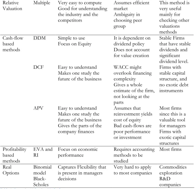
In order to summarize and make a clear decision on the model to use in the exercise of this study, we are going to observe the figure below that sums up the different methods advantages, disadvantages and the situations were ones are used instead of others. This will be very important to select which are the valuation methods that best apply to Vestas characteristics.

(20)

Relative

Valuation Multiple Very easy to compute Good for understanding the industry and the competitors Assumes efficient market Ambiguity in choosing peer group This method is very useful mainly for checking other valuations methods Cash-flow based methods DDM Simple to use

Focus on Equity It is dependent on dividend policy Does not account for value creation

Stable Firms that have stable dividends and significant dividend level.

DCF Easy to understand

Makes one study the future of the business

WACC might overlook financing complexity

Gives a whole estimate of the firm, not looking at the parts Firms with stable capital structure, and no exotic debt instruments

APV Easy to understand

Makes one study the future of the business Gives the parts of the company finances

Assumes that reinvestment yields cost of equity Bad cash-flows are poor performance or investment Most firms since this is a valuable tool for managers Firms with exotic capital structures Profitability based methods EVA and

RI Focus on economic performance Requires accounting methods to be studied Most firms Real Options Binomial model Black-Scholes

Captures Flexibility that is present in managers decisions

Very hard to apply to most companies

Commodities exploration R&D companies

Table 1: Resuming Valuation Methods

2.6. Conclusion

But which of these methods applies to Vestas and its business? Is it necessary to choose one or will the exercise of different valuation methods yields us a more comprehensive firm’s picture? The real option valuation method does not apply since it would be very hard to create a replicating portfolio of the firm industrial activities and different aspects of the business. The company has not paid dividends since the last ten years, and although recently the company CFO has come forward and said that the company will be paying its dividends in a not so distant future, it is not expected that this should be relevant for a company of the business size of Vestas, and so the DDM will not be considered further.

(21)

The model chosen to valuate Vestas will be a DCF analysis that takes into account a reasonable number of scenarios (two scenarios in addition to the base case) to account for the uncertainty that comes from the industry’s cyclicality.

The explicit forecasted period will be the necessary time frame to account for a full business cycle, and the terminal value will be calculated as the average of the explicit period cash-flows. In addition an EVA valuation model will be performed not just to double check the results, but to better understand the value creating process of the company (the same scenarios will be included).

A multiple analyses will also be performed as a check measure. The multiples to be used will rely on forward looking multiples, and based on enterprise value since, as we have seen previously in this chapter, these are the ones that are more accepted by both researchers and investors.

3. Industry Overview

The Wind Energy market has been gaining relevance in the last decade and Vestas has been at the forefront of this growth, alongside General Electric and Siemens. Other companies have been emerging as competitors in some European companies like German Enercom and Spanish Gamesa, as well as some companies in the emerging markets that are supported by these governments like the Indian Suzlon or the Chinese Goldwind. In the graph below we can see the increase in the installed capacity of wind turbines since 1996.

Figure 1: Global Cumulative Installed Wind Capacity, Source - Global Wind Energy Council (GWEC).

This industry is somewhat cyclical, as most manufacturing industries, mainly due to the high level of fixed costs. The industry was impacted by the 2008 financial crisis with a delay of two to three years since the main effect, particularly on Vestas, was felt in 2010 and 2011, not only due to the cyclicality but also due to the increased difficulty in financing large projects. In fact the financial crisis has prompted companies to restructure, decrease fixed costs and increase outsourcing. Vestas has done this restructuring in 2012 and 2013.

Nonetheless the crisis has not stopped the growing trend of demand of wind energy since this has become the most developed and efficient green energy. Additionally, the outlook of the

(22)

wind energy market is positive has it is expected to continue its growth due to the oil and gas becoming more scarce and pricier, continuing the trend observed in previous years. Countries and Governments have also been pushing to be less dependent on fossil fuels, which make the forecasted scenarios look even more encouraging for wind turbine manufacturers.

The industry is also deeply impacted by government policies. Whether it is regulation that favours green energy, international agreements regarding environment protection or subsidies and co-investments given by governments to energy distributors used to build facilities, the growth of the wind energy market is, and has been, strongly tied with politics actions. It is importance to notice that state subsidies have been very important in driving the growth of companies like Vestas that attribute most of their revenue to big projects. This is also evidenced by the recent growth of Chinese producers due to the government effort on decreasing fossil fuels dependency.

In the last decade there has been a growing concern among the worlds’ demographic from the use of green energy as an alternative from not just the fossil fuels, but also the socially condemned nuclear energy. As green energy becomes more popular among consumers wind distributors have been looking to use more renewable energy sources and communicate their “greener” image.

Notwithstanding the popularity of wind energy, there are still some fractions of the population against it, mainly people that live close to wind farms and complain about the effect on the landscape and the noise generated by the turbines.

Another factor that might contribute to the positive outlook on the demand in wind energy is the focus of the producers to invest in research and development, which has been driven by the desire to get an edge over the competition, in order to provide more power/cost efficient turbines. This is also notable by the number of patents that these companies possess. In the long term this expenses should make wind energy more attractive, therefore increasing its demand.

It is also very important to notice that a big part of the expected growth in this industry shall be driven by the increase in demand in emerging markets. This is a very consensual forecast among analysts of the industry, which expect mainly India and China to drive growth. Vestas acknowledges that it does not have a dominant role in these markets, and has made it a goal to increase its share in the emerging markets.

The industry has high entry barriers due to the high fixed costs of that are associated with the manufacturing of the turbines. The main substitutes for wind energy are the fossil fuels that are becoming more expensive and loosing relevance to renewable energy, nuclear energy that has been losing importance due to the negative effects caused by disasters and other green sources, that are not as efficient or with such potential as the wind energy.

(23)

The clients (that distribute wind power) have somewhat strong bargaining power and due to the alternative of turbine producers, while the suppliers have lower negotiation power due to the big number of parts manufacturers. The competition among producers is strong. The biggest players are General Electric, Siemens and Vestas but there are European, Indian and Chinese companies that rose to prominence due to the support of their home governments.

One main limitation is that wind turbines production is still heavily dependent on the wind levels, which can cause overloads in the grid infrastructure of the wind farms. This is one of the reasons for the increase in the importance of offshore wind farms as opposed to the onshore wind farms. In the graph above we can see that although being a fairly new technology, their forecasts for the future are more positive than that of onshore segment. Although the whole industry has positive growth outlooks, the offshore market seems to be increasingly more attractive mainly due to the higher level of wind in these areas and the technological improvements that have made possible the building turbines that are capable of capturing higher wind levels, which require less maintenance and that have higher potency. Vestas has been in a leading position in this high growth segment that has higher barriers of entry than the onshore segment.

The manufacturers of this industry, besides producing wind turbines, provide an array of services different than one might be expecting. In addition to producing, assembling and delivering the wind turbines, most of the producers also provide counselling and overseeing, implement and project planning for optimisation of wind farms, while also providing maintenance and repairs of the grid infrastructure.

Additionally some manufacturers, like Gamesa for example, also manage the wind farms and sell energy to distributors, having a similar role to some of its clients, which is something that

(24)

Vestas has always shied away from, considering itself solely as a wind turbine manufacturer. However Vestas has announced a renewed emphasis on making services more profitable on the Capital Markets Day of 2014.

All in all, the wind energy market is an attractive industry mainly due to its positive growth outlook, and the both the economic agents preference for green energy coupled with the developed technology of the wind turbines that make this the most efficient green source. Nonetheless the cyclicality of the business and the fact that it is heavily dependent on government support and policies add to the riskiness of the industry.

Additionally these industry players have high R&D expenses to allow them to be at the forefront of wind turbine making technology and differentiate them in this way and to be able to find the best cost/power efficient turbine possible as well as new ways to transport or setup a wind farm to better capture the full capacity of the wind.

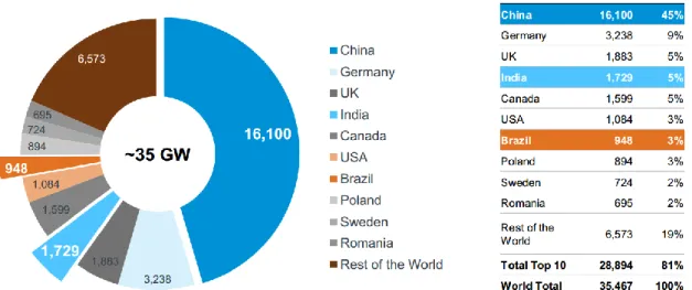
Finally it is crucial to notice the importance of the emerging markets penetration in order fully capture the growth that will be experienced in the industry in the following years. In the figure below, taken from a presentation of Vestas Capital Markets Day, we can see that India, China and Brazil account for more than 50% of the wind capacity installations in 2013, a trend that is expected to continue.

Vestas identifies the dominance of these markets as an important step to maintain its position as a global leader, both in its Capital Markets Day and in the presentation of its half-year report of 2014

Figure 3: Wind Capacity Installations in 2013, Source: "Grow profitability in mature and emerging markets", Capital Markets Day; 2014, June 12.

(25)

4. Vestas Wind Systems A/S 4.1. The Company

Wind. It means the world to us.

Vestas was the world pioneer in wind turbine manufacturing and still is one of the world leaders in this fast growing industry. But this has not been a clear path from the local Danish company that started as a small blacksmith in a small town in Denmark called Lem, in 1989. Establishing credibility with the production of window steel frames the brand grew and by 1968 the company was exporting hydraulic cranes for 65 countries.

After the first oil crisis, people became more aware of the relevance of clean sources of energy. Vestas started to study the potential of turning wind into electricity and the Danish government was very supportive, which led to the first wind turbine produced by the company in 1979. In 1987 Vestas decides to focus solely on wind energy, and making it a possible alternative for traditional, and not clean, energy sources.

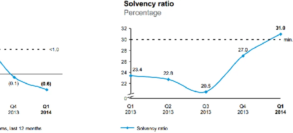
In 1995 Vestas develops one of the world’s first offshore wind farm, and sees the potential of this segment. The company has been dominating the fast growing wind energy market and in 1998 Vestas goes public and it is listed in the Copenhagen Stock Exchange ever since. Since then Vestas has been growing and, despite having lost significant amount of market share since 2007, mainly to new competitors from emerging markets. Meanwhile they had been recovering market share having 20% of the world’s installed capacity, and 30% of the offshore capacity. The last financial crisis had an impact on Vestas and made emerge a necessity for restructuring the operations of the firm as well as its solvency situation. Therefore the company has been undergoing the restructure process mainly focusing on decreasing fixed costs, mainly through the disposable of non necessary assets. Also important to notice are the targets for solvency announced by Vestas in terms of Solvency ratio (higher than 30%) and Net Debt to EBITDA (lower than 1), which can be seen below.

(26)

In accordance with this low fixed costs policy Vestas has entered in a joint venture with Mitsubishi Heavy Industries Ltd specially directed at attaining and maintaining the global leadership of the offshore wind segment. The company believes that this Joint Venture coupled with a new turbine the V164-8.0MW, which was designed to be able to capture the high offshore wind levels while providing the cost efficiency and requiring low maintenance, will allow the company to achieve this goal.

Additionally it is important to notice that Vestas, like its competitors, has high R&D investments in order to be at the forefront of the industry and be able to provide the best cost efficient turbines, which is evidenced by the number of research centres. However since 2012 there has been a reduction in R&D costs, with a lot of research facilities being closed.

The 2013 and 2014 2nd Quarter showed an improvement in performance in terms of revenues and operating expenses in addition to having met its self imposed solvency targets, which indicates that Vestas efforts to restructure operations seem to have put the company in a good financial and operational position to respond the growth demands that are expected in the industry’s positive outlooks.

Finally one cannot forget that Vestas is, as wants to remain, the most recognized brand in the wind turbine manufacturing business being associated with innovation and reliability. The company wants to enhance this image as is evidenced, for example, by the recently announced sponsoring of the team Vestas Wind in the Volvo Ocean race. In fact the company CEO stated that the competition is a “perfect match for us to engage with our customers, showcase our technology and strengthen our brand” 9 adding that it supports the company’s corporate strategy of “Profitable Growth”.

4.2. The Outlook

Vestas is a much admired company in Denmark and the Scandinavian countries being one of the most successful companies coming out of the area. Its business experience has made it a known name in the wind turbine business not just in the markets it dominates Europe and North America as also by the markets where Vestas has less expression like the Asian markets. The new strategy of Vestas focuses on four focal points, being the first is to grow profitably in mature and emerging markets. As mentioned previously, the company wants to increase its market share in emerging market in addition to maintaining its position in its other markets. The company strongly believes in its customer relations and has made efforts position it globally to be able to access these markets.

9_{“Vestas brings passion for the wind to ocean racing, enters Volvo Ocean Race 2014-2015 with first-ever}

(27)

Secondly the company will focus on better capturing the full potential of the service business, mainly project planning and plant management. Vestas plans to establish a new service organization with direct report to the CEO and bundle its service business in all new orders. Thirdly, is to reduce the Levelised Cost of Energy (LCoE). This means that Vestas will focus on, not just having the most cost efficient wind turbine in the market, but to make wind energy has affordable as other energy sources. This measure, the LCoE, as been decreasing yearly, but the company wants to decrease it at a faster rate than the market, mainly trough innovation. Lastly, but probably most importantly, is Vestas will to diminish operating expenses to a much lower level than they were in previous years. As mentioned previously it can be seen that in the 2nd Quarter of 2014 this is already producing effects, mainly due to the reduction of the number of workers the disinvestments in some factories that are replaced by 3rd party production among other measures.

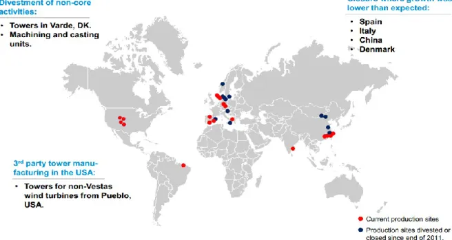
Vestas believes that with less production, but close relationship with suppliers for quality control, it can be more flexible and therefore it should be able to better adapt to the business cycles. In the figure below we can see the disinvestment made by the company that reduces from 31 world factories to 19.

Figure 5: Source: "Improve in operational excellence", Capital Markets Day; 2014, June 12.

Vestas believes that these four points will allow the company to increase its market share as well as increase its profitability by reducing operating expenses. The significant improvement in operational efficiency is notable in the company’s recently published results, but it remains to be seen that Vestas can increase market share in emerging markets where there are already established companies in the industry like India (Suzlon) and China (Goldwind, among others).

(28)

Strategy and market outlooks aside, Vestas Chief Financial Officer, Marika Fredriksson, has announced plans that are directly tied to shareholders interests. In February of 2014, the company declared it was closer to paying a dividend of about 30% of annual net results, with the contingency that the company solvency targets, mentioned earlier, are met.

4.3. The Peer Group

The peer group selection is the most important part when conducting multiples valuation. In the case of Vestas it is very hard to find a suitable group mainly due to the nature of the industry’s competitors.

The companies that have as much global brand awareness as well as international business volume are parts of bigger groups and so they cannot be used in relative valuation. These are General Electric Wind and Siemens Wind Energy. The former has been the biggest challenger of Vestas for the wind energy turbine market, while the later has lost relevance in the previous years but is still one of the biggest manufacturers in the market.

There are some relevant European competitors although these fail to capture the global business that Vestas captures. These companies are fairly smaller and were able to penetrate the market due to the support of their respective governments. The Spanish Gamesa and the Swedish Nordex are both listed companies and have similar business model to Vestas, and despite being much smaller than the company we are studying, will be included in the peer group. The German Enercom is similar to these but is a private company.

Additionally there are some companies that are similar to the European ones described above but are from emerging market. The already mentioned Indian Suzlon and Chinese Goldwind are wind turbine manufacturers that have great expression in their respective countries and benefited from political support. These are both listed companies that have a smaller revenue volume than Vestas. Both these companies will be used in the peer group.

So from the paragraphs above we can see that the peer group is constituted by four companies that are fairly smaller than Vestas (Gamesa, Nordex, Suzlon and Goldwind). Ideally General Electric Wind and Siemens Wind Energy, maybe in conjunction with the European countries, would form a suitable peer group but as these are part of bigger groups they cannot be used. As the peer group is not the most suitable, one should take multiples valuation as just a way to triangulate results and not as a standalone valuation technique, as we have already mentioned in the peer review segment.

5. The Weighted Average Cost of Capital

In this chapter we will focus on calculating the Weighted Average Cost of Capital (WACC). As we have seen previously we know that to calculate this discount rate that will be used in the DCF valuation one needs first to calculate its inputs. This section is dedicated to the

(29)

methodology and assumption behind the calculus of the Cost if debt, the market risk premium, the risk free, the cost of equity, so we can finally calculate the WACC.

5.1. The Cost of Debt

There are several approaches to estimate the cost of debt. When a company has bonds that are listed on an exchange, then one can see the yield and have the cost of debt for those, if the bonds have a medium term one can use that yield as a cost of debt. Alternatively, when with a high number of bonds one can do an average of the yields to get the cost of debt. Neither was the case with Vestas that has one publicly traded bond with a short term maturity.

Another approach is to use the rating of a company and then consult a rating table, which will indicate us a proxy for the cost of debt of a company. These scores are normally given by the rating agencies that follow and analyze the companies’ creditworthiness and solvency outlooks. There are no rating agencies following Vestas.

Therefore Vestas rating was calculated using a tool that is available in Damodaran website. This is an excel spreadsheet that needs some inputs regarding the company’s activity and yields a rating. The inputs are highlighted in the table below.

Input Value Explanation

Type of firm Large

Manufacturing Firm

Vestas is in its essence a manufacturing firm and can be considered to be large

Current Ebit € 123 m This should be an average of the last periods if the company does not have stable cash flows. In Vestas case it was used the average from 2009 to 2014. Current Interest Expenses € 90 m As with the Ebit, this could be an average of the last

periods. In Vestas case it was used from 2012 to 2013, because this better reflects the financial stability of the firm.

Risk free 1,24% This is the same risk free as we use for the WACC of the project.

Table 2: Cost of Debt Inputs' Assumptions

These inputs yield a rating of an interest coverage ratio of B- which yields an estimated cost of debt of 8,49%. Now we need to calculate the after tax cost of debt, which is just the cost of debt without the effect of the effective tax rate. The final after tax cost of debt is then 6,12%. The assumptions behind the risk free rate will be seen next.

5.2. The Risk Free Rate and Market Risk Premium

Before computing the cost of equity, it is necessary to establish some assumptions about the risk free and market risk premium calculations, as was previously mentioned in the literature review section

For the risk free rate one should use the risk free rate of the currency of the country where the company is from. However, in the case of Vestas, and due to the fact that this is a company

(30)

that is global in its business, as evidenced by the presentation of its official reports in Euros, it should not be used the Danish risk free. This, coupled with the stable exchange rate between the Euro and the Danish Krone, while being a company that has the most of its revenues outside of Denmark contributes to the choosing of the of the risk free rate of the Euro.

The closest to a Euro currency risk free rate should be a German government bond index, with a maturity of ten years because that is closer to the explicit period. So GDBR10 Index was used with monthly data from January 2009 until June 2014. As this is an index the returns are annualized and we need to transform them into monthly frequency. As mentioned in the Literature Review, this should be a date at a point in time and not an average of a period. The date chosen was 30th June of 2014 to which corresponds an annualized rate of 1,24%.

The market risk premium as further considerations to make, but the rationale is the same. Although usually one should use the market were the country is situated, in the case of Vestas that is a global company, Koller et al (2005) states that a good alternative should be one of the MSCI indexes. As the majority of Vestas activity is in Europe, the MSCI Europe Index was chosen as a proxy for the market returns.

Again monthly data was taken from January 2009 to June 2014. Monthly data was used to decrease the autocorrelation among observations, as explained in the literature review, and the period was chosen to reflect the current state of the market, without the effects of the last financial crisis(for this purpose the data for the market risk premium will not include 2009 since the market was very much affected as a whole). The annualized historical average for this period is 4,25%. Although this seems a fairly low number for the market risk premium, it should be noted that historically Germanic and Scandinavian markets have had low risk premiums.

5.3. The Cost of Equity

As mentioned previously when reviewing the valuation models, to compute the cost of equity one as to assume an asset pricing model. In this case the CAPM was chosen as this is the most widely accepted model. The equation for this model is stated below.

Ke = rf+ βe∗ MRP

Since we already have in the previous sub-section the risk free rate and the market risk premium, we are only missing the Beta of the company. To get this we need to regress excess returns of the company (Ke − rf) by the market risk premium. Again the data selected was

similar to the one for the market risk premium mainly for the same reason (to assure there is no autocorrelation among observations) and to be consistent (Only using the data from 2009). This yields a beta equal to 1,43. The beta measures the correlation of the market volatility with the company volatility. And as we can see the volatility of the company is far less smooth in

(31)

relation with the market. This high also reflects the cyclicality of Vestas business, which adds to its volatility and therefore will yield a higher cost of equity.

Now that we have all the inputs to fill the equation above we can compute the cost of equity and it yields us a result of 7,33%.

5.4. The WACC

We have almost all the inputs necessary to calculate the WACC, using the formula that was previously described. However we know that Vestas does not have mixed instruments in its capital structure, and so the formula will be simplified as the one given below.

WACC = D

D + E∗ rd ∗ 1 − t + E D + E∗ re

So the only missing inputs are the weights of equity and debt and for this we need to find the company’s capital structure. For this we need to know the current company value of equity and debt at market value. The current market value of equity is just the number of outstanding shares multiplied by the share price, which yields an equity value of € 56.870 m, as of 18th July 2014.

The current market value of debt is more challenging to find. For the publicly traded bond we just need to use the value at which the bond is being traded. For the short term loans we can assume that book value equals the market value. F

or the medium to long term debt, that in the case of Vestas is just one outstanding loan, I will use the interest paid on the loan and dived by the new calculated cost of debt and therefore get the market value of the long term loan. Summing the value of the parts of debt we get the current market value of the debt of € 9.857 million.

With this we have an approximated capital structure and therefore the weights of 14,77% and 85,23%, of debt and equity respectively. In order to understand if this was Vestas target capital structure, the historical capital structure was analyzed.

It seems that besides 2012, where the company went through a major restructuring process, the capital structure as been fairly stable, being that the average has been of about 16%. It is interesting to see that the peer group, despite following the same fluctuations, seems to have historically more debt than Vestas, about more 10% which is a significant difference.

Equity valuation : Vestas Wind Systems A\S