Myocardial partial volume correction of internal left ventricular structures in emission tomography images

(1)

FACULDADE DE CIÊNCIAS

DEPARTAMENTO DE FÍSICA

Myocardial partial volume correction of internal left

ventricular structures in emission tomography images

Mauro Santana Costa e Sousa

Orientadores

Dr. Kris Thielemans, Institute of Nuclear Medicine, University College London,

London, UK

Prof Dr. Pedro Almeida, Instituto de Biofísica e Engenharia Biomédica, Departamento

de Física da Faculdade de Ciências da Universidade de Lisboa, Lisboa, Portugal

MESTRADO INTEGRADO EM ENGENHARIA BIOMÉDICA E BIOFÍSICA

PERFIL: RADIAÇÕES EM DIAGNÓSTICO E TERAPIA

DISSERTAÇÃO -2016-

(2)

(3)

FACULDADE DE CIÊNCIAS

DEPARTAMENTO DE FÍSICA

Myocardial partial volume correction of internal left

ventricular structures in emission tomography images

Mauro Santana Costa e Sousa

Dissertação Orientada por Doutor Kris Thielemans e Professor Doutor

Pedro Almeida

Mestrado Integrado em Engenharia Biomédica e Biofísica

Perfil em Radiações em Diagnóstico e Terapia

(4)

(5)

i | P a g e

Acknowledgements

I would like to express my appreciation towards my supervisor, Dr Kris Thielemans, who has been extremely supportive and for recognising the difficulties associated with the completion of this text. I would also like to thank Dr Brian Hutton for the wonderful opportunity of being able to take part of his team at the Institute of Nuclear Medicine, University College London Hospital. My thanks are also extended to my internal dissertation supervisor, Professor Dr Pedro Almeida, for his unconditional support, despite the distance.

My sincere appreciation goes to my colleagues at the Institute of Nuclear Medicine, Débora Salvado, Richard Manber, Hasan Sari, Beverley Holman, Alexandre Bousse, Kjell Erlandsson, Vesna Cuplov and Ottavia Bertolli, who have been always supportive and ready to help. A very especial thanks goes to Cristina Campi, Maria Zuluaga (UCL Centre for Medical Image Computing) for the kind input of their cardiac segmentation methods in this work. I also thank Simon Wan and John Dickson for the very useful discussions and input provided during this project.

I would like to express my special thanks to my fellow colleagues and professors at Institute of Biophysics and Biomedical Engineering, at University of Lisbon: Professor Dr Nuno Matela, Professor Dr Alexandre Andrade, Melissa Botelho, Rui Santos, Danielle Batista, David Soares and Nuno Silva; without whom my academic experience would not have been as rich.

To all the friends I met in London, António Ferreira, João Monteiro, Nino, Dona Maria José & family, Xaverito & family, my colleagues at IXICO and most importantly Sérgio & Lisete, I deeply appreciate all the encouragement towards helping me completing my thesis and all their help during the first months in London.

Last, but definitely not least, my greatest appreciation goes to my family, my mother, my brother, and my soon-to-be wife and son, André. This thesis is dedicated to you all, who sacrificed a lot for me to be able to complete my project and dissertation. For that and for your continuing support, I will be eternally grateful.

(6)

ii | P a g e

Resumo

A imagiologia médica apresenta-se como sendo um conjunto de processos que levam à criação de representações visuais do interior do organismo para análise clínica e/ou auxílio em processos de intervenção médica.

Desde o seu aparecimento e aplicação prática que a imagiologia tem tido um impacto significativo na sociedade, permitindo a confirmação de condições patológicas, possibilitando a avaliação e planeamento de tratamentos, e o fornecimento de uma alternativa a métodos invasivos e, essencialmente, constituindo práticas que permitem o diagnóstico prematuro de patologias. Todos estes aspetos fazem com que a imagiologia médica contribua, em última instância, para a diminuição da taxa de mortalidade e para o aumento da esperança média de vida das populações. No entanto, apesar dos mais de 100 anos de história desde o aparecimento das primeiras técnicas imagiológicas, existem ainda inúmeros desafios por ultrapassar no campo da imagiologia médica. Uma das principais motivações é a otimização de processos de diagnóstico em fases prematuras de diagnóstico, o que possibilita um maior leque de ações terapêuticas, podendo fazer a diferença no resultado final do tratamento dos pacientes.

Esta necessidade, aliada ao facto de a maior causa de mortalidade a nível mundial ser devido a doenças cardiovasculares (Allender et al. (2008), Lloyd-Jones (2010)), justifica uma prioridade na investigação de metodologias que visem o diagnóstico de patologias do foro cardíaco num estado em que as ações preventivas e de tratamento permitam uma maior eficácia final para benefício do paciente.

Em particular, as modalidades de imagiologia médica podem distinguir-se entre métodos morfológicos (ou anatómicos) – que visam a obtenção de informação anatómica do organismo -, e métodos funcionais (ou de emissão), que têm por objetivo quantificar, de modo não invasivo, processos fisiológicos e metabólicos ocorrentes no organismo.

Porém, embora este último tipo de métodos apresente uma maior sensibilidade e especificidade na deteção de fenómenos fisiológicos, ao nível molecular, tal surge em detrimento da resolução espacial das imagens. Este fenómeno de degradação da resolução espacial, mais acentuado em imagens funcionais, é conhecido como o efeito do volume parcial. Apesar de ser um tópico sujeito a grande foco de investigação na área imagiológica médica, o efeito do volume parcial não tem, na prática, uma metodologia suficientemente versátil e eficaz de correção.

Os mecanismos de correção do efeito do volume parcial baseiam-se essencialmente na implementação de processos de restauração do desfoque de imagem, havendo uma redistribuição de atividade dos objetos de volta à sua localização original.

(7)

iii | P a g e metodologias de correção do efeito to volume parcial necessitam, na sua maioria e de forma a serem mais eficazes, de informação imagiológica funcional e morfológica, correspondentes. É de notar a complexidade associada a este género de processos, uma vez que incorrem num número de diferentes passos de processamento consecutivos, entre eles a segmentação de regiões de interesse, o co registro de imagens funcionais e anatómicas, e implementação do processo de correção propriamente dito, sendo que este pode ser efetuado sob o ponto de vista da imagem final ou durante a reconstrução de projeções tomográficas. Desta forma, é possível definir restrições geométricas que auxiliam no processo de compensação deste efeito.

Por outro lado, o coração possui estruturas intraventriculares, os músculos papilares e as trabéculas, que se caracterizam por serem protrusões das paredes miocárdicas ventriculares, de massa apreciável e que servem o propósito de ancorar as válvulas auriculoventriculares de forma a impedir a regurgitação sanguínea para as aurículas, durante a diástole auricular/sístole ventricular.

A questão em foco é que metodologias de correção do efeito do volume parcial aplicadas ao aparelho cardíaco utilizadas na bibliografia ignoram a atividade produzida por estruturas intraventriculares, considerando-as como pertencentes à “blood pool”, que se situa na cavidade ventricular, sendo que este passo é feito de forma a simplificar a rotina de correção, minimizando o número de estruturas cujo efeito do volume parcial se pretende corrigir, tomando apenas em consideração uma parede miocárdica e uma “blood pool”, na grande maioria dos casos.

O objetivo do projeto corrente foi a avaliação sobre se a melhor opção residiria na tomada de consideração destas estruturas intraventriculares como fontes independentes produtoras de efeito do volume parcial a um nível significativo, ou se o seu efeito de desfoque seria desprezável ao ponto deste ser mascarado pela atividade da “blood pool”.

De forma a testar esta ideia, projetámos um processo lógico dividido em três instâncias de complexidade crescente. A primeira abordagem consistiu num estudo exploratório caracterizado pela modelação de um sistema cardíaco, seguido por um procedimento de desfoque simples do mesmo, através da convolução do modelo com uma função de dispersão típica de um sistema de tomografia por emissão, e posterior avaliação do efeito de volume parcial produzido por estruturas intraventriculares. O objetivo desta abordagem foi o de determinar se o efeito de volume parcial produzido por estruturas intraventriculares seria significativo ou não, sendo que tal foi efetuado por comparação com o efeito correspondente produzido pela “blood pool”, referida na literatura como uma estrutura relevante no processo de desfoque imagiológico. Mediante a potencial determinação de que o efeito produzido pelas estruturas internas ventriculares seria efetivamente significativo e tendo em conta as simplificações efetuadas durante a criação do modelo, um estudo mais aprofundado deste efeito justificar-se-ia.

É neste sentido que surge a segunda abordagem ao problema, que consiste no aumento da natureza realística do processo de determinação do efeito de volume parcial produzido pelas estruturas intraventriculares, através da utilização do STIR (Software for Tomographic Image

Reconstruction). O STIR é um programa que permite simular o processo de reconstrução de

imagens tomográficas, dotando as mesmas de um padrão de desfoque e de ruído realistas. A determinação de uma potencial enfatização do efeito produzido por estruturas internas ventriculares justificaria um ainda maior aprofundamento do estudo deste efeito.

Neste contexto, surge a terceira e última instância deste estudo, que corresponde à levada a cabo de estratégias de correção de efeito do volume parcial propriamente ditas. O principal resultado produzido por este estudo seria a determinação do erro obtido ao recuperar a distribuição de

(8)

iv | P a g e regiões de interesse. O resultado final baseou-se na determinação de que, segundo as simplificações utilizadas na criação do modelo, as estruturas intraventriculares produziriam um efeito local significativo sobre a parede do ventrículo esquerdo, podendo efetivamente mascarar lesões hipo-activas ou adelgaçamentos patológicos da parede do ventrículo, em locais adjacentes à estrutura intraventricular em questão.

É de referir que o presente estudo constitui uma primeira aproximação à avaliação do efeito do volume parcial produzido por estruturas intraventriculares, sendo que até à data, não há conhecimento de um estudo semelhante.

Como conclusão final, e à luz das simplificações adotadas durante a execução deste estudo, não existem indícios que apontem para o facto de estas estruturas não serem relevantes, pelo menos a nível local. No entanto, há que compreender que, de forma a obter uma noção mais completa e precisa sobre a relevância destas estruturas intraventriculares, um estudo adicional terá de ser realizado de forma a comprovar a importância de estruturas internas ventriculares num ambiente clínico, e em particular, se estas devem ou não ser consideradas como independentes.

Palavras-chave: Efeito do volume parcial; Correção do efeito do volume parcial; Estruturas

(9)

v | P a g e

Abstract

Introduction: In emission tomography, the system’s limited spatial resolution leads to

three-dimensional image blurring, a phenomenon called partial volume effect (PVE). This limited resolution gives rise to activity spillover between regions in the imaged object, resulting in significant changes in the measured image activity distribution, which is particularly evident in structures with small dimensions. Hence, precise quantification based on image activity values depends on a rigorously implemented partial volume correction (PVC) routine. In nuclear medicine images some PVC methodologies make use of corresponding morphological images in order to provide additional information which assist in the correction procedure. This approach is popular in cardiac emission data. However, in the current PVC literature, cardiac intra-ventricular structures (IVS), namely papillary muscles and trabeculae carneae, have been largely ignored, while they may potentially produce a significant influence in terms of activity spillover.

Methods: A progressively more complex set of simulation steps were involved in this study to

investigate the partial volume effect of IVS. The first step involved the study of a simple blurring model using Matlab, which evolved into a model with a more realistic nature by using STIR (Software for Tomographic Image Reconstruction), which in turn evolved to the evaluation of an actual PVC methodology using C++ and Matlab scripts for PVC. A diastolic right and left ventricle model, designed according to a 17 segment division (Cerqueira et al. (2002)) was constructed, and the PVE originated from the IVS was assessed in all the individual segments of the left ventricle, throughout all the tested approaches. This IVS PVE influence was then compared to the blood pool’s (BP) spillover, since the latter is an already well established effect studied in the current literature.

Results: The results obtained showed some agreement between the various simulation

approaches utilized, showing that the total PVE produced by the overall IVS was comparative to that of the blood pool, but this could still be accounted for in PVC methodologies that do not consider IVS. However, the results consistently pointed to the fact that in local terms the IVS produces an effect that surpasses that of the BP, and PVC methodologies that do not take the IVS into account are not able to adequately recover the initial object’s activity distribution, locally.

Conclusion: It was shown that the local PVE of the IVS over the left ventricle wall was

significant, which can potentially have an effect in terms of masking or over emphasizing anomalous uptakes in regions of the myocardial wall that are in the vicinity of IVS.

(10)

vi | P a g e

Table of Figures

Figure 2.1 - PET imaging principle: positron-electron annihilation and subsequent emission of two 511 keV photons in opposite directions, and respective photon coincidence detection by

PET detectors (Weirich & Herzehog, 2012) --- 4

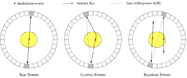
Figure 2.2 - Different types of coincidences: Left) True event; Centre) Scatter event; Right) Random event (Weirich & Herzehog, 2012) --- 5

Figure 2.3 - Left) 82_{Rb-chloride myocardial perfusion study with no attenuation correction;} Right) Corresponding study with attenuation compensation (Di Carlie & Lipton, 2007) --- 7

Figure 2.4 - Left) Non-corrected (raw) Rb-82 cardiac image; Centre) Corresponding scatter map; Right) Scatter corrected image (de Kemp and Nahmias, 1994) --- 8

Figure 2.5 - Illustration of the PVE phenomenon (Soret et al. 2006) --- 9

Figure 2.6 - Illustration of back-projection resulting images, with different numbers of projections (Platten, 2003) --- 12

Figure 2.7 - Iterative Reconstruction Process (Cherry et al. 2003) --- 14

Figure 2.8 - Open view of the LV free wall: PM and TC (Moore et al. 2010) --- 17

Figure 2.9 - LV 17 segment model (Cerqueira et al. 2002) --- 18

Figure 2.10 - General relationship between LV 17 segment model and myocardial regions (Groch & Erwin, 2001) --- 19

Figure 2.11 - Illustration of a vertical long axis LV view with the depiction of the apical cap (Cerqueira et al. 2002) --- 19

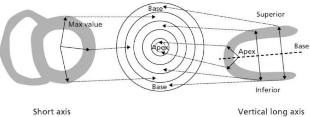
Figure 2.12 - Illustration of a mid-cavity short-axis heart view (Cerqueira et al. 2002) --- 20

Figure 2.13 - Illustration of a horizontal long axis heart view (Cerqueira et al. 2002) --- 20

Figure 3.1 - Illustration of Yang's PVC method in 1 dimension (Erlandsson et al. 2012) --- 28

Figure 4.1 - 3D Ventricular Heart Model --- 33

Figure 4.2 - Three referential views of the ventricular heart model. Left) mid-cavity short axis; Centre) horizontal long axis; Right) vertical long axis. --- 33

Figure 5.1 - IVS Diameter Study --- 40

Figure 5.2 – Local IVS-LV wall separation study --- 41

Figure 5.3 - Total IVS-LV wall separation study --- 42

Figure 5.4 - Local LV wall thickness study --- 43

Figure 5.5 - Total LV wall thickness study --- 43

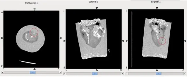
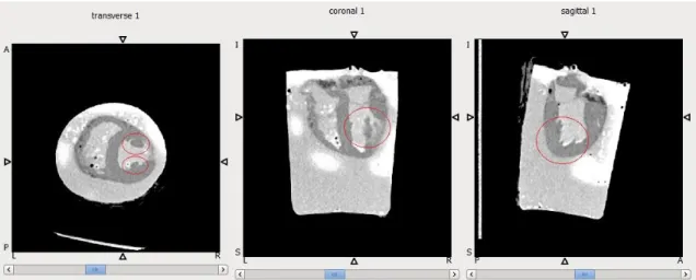
Figure 5.6 - CT scan of excised dog heart #1 – 3 reference views --- 45

Figure 5.7 - Zoomed view of excised dog heart #1 – more superior axial and coronal views --- 45

Figure 5.8 - Apical location of excised dog heart #1 - all 3 reference views --- 46

Figure 5.9 – Zoomed view of excised dog heart #2 – axial and coronal views --- 46

Figure 5.10 - Apical location of excised dog heart #2 - all 3 reference views --- 47

Figure 5.11 – Additional representation of excised dog heart #2 – all reference views --- 47

Figure 5.12 – CT scan of excised dog heart #3 – 3 reference views --- 48

(14)

x | P a g e

Figure 5.15 – Axial 1D profile location illustration --- 53

Figure 5.16 – Cardiac model profile averaging. Number of noise realizations = 2 --- 53

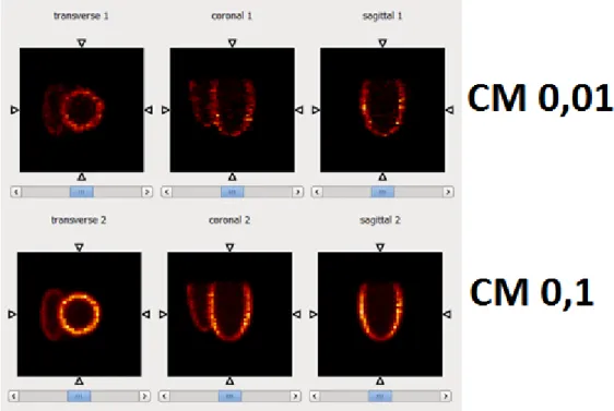
Figure 5.19 – FHWM Variance with CM in the representative XX direction --- 55

Figure 5.20 – FWHM of PSF of 100 FBP reconstructions of point sources with CM of 0.01 --- 56

Figure 5.21 - FWHM of PSF of 100 FBP reconstructions of point sources with CM of 0.01 – truncation of outliers --- 56

Figure 5.22 – Amended graphical representation of FWHM Variance with CM in the (representative ) XX direction --- 57

Figure 5.23 – FHWM Variability along the YY direction of the FOV, using an OSEM reconstruction --- 58

Figure 5.24 - FHWM Variability along the XX direction of the FOV, using an OSEM reconstruction --- 59

Figure 5.25 - FHWM Variability along the YY direction of the FOV, using a FBP reconstruction 60 Figure 5.26 - FHWM Variability along the XX direction of the FOV, using a FBP reconstruction 61 Figure 5.27 – Depiction of OSEM reconstructed images with different numbers of subiterations --- 62

Figure 5.28 – Maximum voxel size variation with number of OSEM subiterations – lower scale --- 63

Figure 5.29 – Blur matching process for STIR reconstructed images --- 64

Figure 5.30 – Axial 1D profile location illustration --- 65

Figure 5.31 – Blur match study of FBP and OSEM reconstructions against 10 mm blurred model image – before matching --- 65

Figure 5.32 – Blur match study of FBP and OSEM reconstructions against 10 mm blurred model image – after matching --- 66

Figure 5.33 – STIR’s IVS Diameter Local PVE Study --- 67

Figure 5.34 – STIR’s IVS-LV Wall Separation Local PVE Study --- 68

Figure 5.35 – STIR’s LV Wall Thickness Local PVE Study --- 68

Figure 5.36 - STIR’s LV Wall Thickness Total PVE Study --- 69

Figure 5.37 –Total PVE Quantification of BP and IVS, under a simple convolution, FBP and OSEM approaches --- 70

Figure 5.38 - Local PVE Quantification of BP, PM and TC, under a simple convolution, FBP and OSEM approaches --- 71

Figure 5.39 - PVC Error following a GTM activity recovery routine --- 74

Figure 5.40 – Original (A), Blurred (B), and Recovered (C) simply convolved images following iY PVC --- 76

Figure 5.41 – Depiction of the variation of the mean activity in the LV, in function of the number of iterations in the iY routine, with associated ROI standard deviation --- 78

Figure 5.42 –PVC Error following an iY activity recovery routine --- 79

Figure 5.43 – Short axis view of the iY PVC routine applied without taking IVS anatomical reference into account. Left) Convolution; Middle) OSEM with 100 averaged reconstructions; Right) FBP with 100 averaged reconstructions --- 80

Figure 5.44 –Atlas based cardiac segmentation technique’s results, on selected CTA data (A – Original CTA image; B – Original CTA Image + Cardiac Segmentation --- 81

(15)

xi | P a g e Figure 5.46 – Results from LV segmentation with active contour technique – 2D inclusion of aorta in vertical long axis view --- 83 Figure 5.47 – Results from LV segmentation with active contour technique – 3D inclusion of aorta --- 84 Figure 5.48 – Depiction of IVS inclusion on BP’s segmentation, in heart A --- 84 Figure 5.49 – Depiction of IVS inclusion on BP’s segmentation, in heart B --- 85 Figure 5.50 – Depiction of inclusion of basal region of IVS in LV’s segmentation, in heart B --- 85

(16)

xii | P a g e

List of Tables

Table 5.1 - IVS and BP PVE Summary from simple convolution blurring study ... 44

Table 5.2 – Number of Total, Random and Scatter counts determination summary ... 52

Table 5.3 - FWHM variation with CM, in the XX and YY directions... 55

Table 5.4 - Amended FWHM variation with CM, in the XX and YY directions ... 57

Table 5.5 - Mean and standard deviation of FWHM values along YY direction of the FOV, using an OSEM reconstruction ... 58

Table 5.6 - Mean and variability of FWHM values along the XX direction of the FOV, using an OSEM reconstruction ... 59

Table 5.7 - FWHM variability along the YY direction of the FOV, using a FBP reconstruction ... 60

Table 5.8 - Mean and variability of FWHM values along the YY direction of the FOV, using an FBP reconstruction ... 61

Table 5.9 – Post smoothing filter’s XX, YY and ZZ FWHM components for FBP and OSEM 64 Table 5.10 - GTM PVC results on an image with a known blur of 10 mm FWHM symmetrical PSF ... 72

Table 5.11 - GTM PVC Error Assessment, upon not including IVS in the correction ... 73

Table 5.12 - iY PVC results following correction of ventricular heart model ... 77

(17)

xiii | P a g e

List of Abbreviations

AHA American Heart Association

APD Avalanche photodiode

BGO Bismuth Germanate

BP Blood Pool

CM Count Magnitude

CSF Cerebrospinal Fluid

CT Computed Tomography

CTA Computed Tomography Angiography

DICOM Digital Imaging and Communications in Medicine

ECG FBP

Electrocardiography Filtered Back-Projection

FDG Fludeoxyglucose

FOV Field of View

FT Fourier Transform

FWHM Full Width at Half Maximum

GE General Electric

GM Grey Matter

GTM Geometric Transfer Matrix

IVS Intraventricular Structure

iY Iterative Yang

LOR Line of Response

LSO Lutetium Oxyorthosilicate

LV Left Ventricle

MG Muller-Gartner

MLEM Maximum Likelihood Expectation Maximization

MRI Magnetic Resonance Imaging

MTC Multi-target Correction

OSEM Ordered Subsets Expectation Maximization

PET Positron Emission Tomography

PM Papillary Muscle

PSF Point Spread Function

PVC Partial Volume Correction

PVE Partial Volume Effect

RBV Region Based Voxel-wise

RC Recovery Coefficient

ROI Region-of- Interest

RV Right Ventricle

SNR Signal-to-noise Ratio

SPECT Single Photon Emission Computed Tomography

STIR Software for Tomographic Image Reconstruction

SUV Standard Uptake Value

(18)

(19)

1 | P a g e

Introduction

1.1. Project Framework

This dissertation was submitted for the purpose of fulfilling my Master’s Degree in Biomedical Engineering and Biophysics – profile in Radiation in Diagnosis and Therapy, at the Faculty of Sciences of the University of Lisbon (FCUL).

The project that led to the writing of the thesis was performed under the scope of the LLP/Erasmus Programme, a European Union (EU) student mobility scheme that provides foreign exchange learning and internship options for EU students. The project was a collaboration between the Institute of Nuclear Medicine (INM), University College London (UCL), London, United Kingdom (UK), and the Institute of Biophysics and Biomedical Engineering (IBEB), FCUL, Lisbon, Portugal.

IBEB focuses on research and post-graduate teaching functions. In addition to Masters and PhD project supervision, IBEB has founded a BSc+MSc programme in Biomedical Engineering and Biophysics. The main research areas at the institute are distributed along 4 main thematic lines: Medical Imaging and Diagnosis; Brain Stimulation and Rehabilitation; Brain Dynamics and Connectivity and Cancer Therapy and Drug Delivery.

Regarding the Research Physics Group at INM, it mainly focuses on Medical Physics applied to Nuclear Medicine and Molecular Imaging. The research projects under way at the institute fall essentially under the scope of emission tomography. The areas of interest are optimized tomographic reconstruction for PET (Positron Emission Tomography) and SPECT (Single Photon Emission Tomography), motion and partial volume image corrections, and multi-modality image analysis applied to clinical research studies in Nuclear Medicine, in particular using combined PET-CT (PET coupled with Computed Tomography), SPECT-CT and PET-MRI (PET coupled with Magnetic Resonance Imaging).

This project consisted in assessing the partial volume effect (PVE) influence of internal ventricular structures (IVS) over the left ventricle wall, in order to ultimately ascertain whether these structures should be taken into account in Partial Volume Correction (PVC) methodologies applied to emission tomography, and in particular to PET. The thesis was performed under the external supervision of Dr Kris Thielemans, Senior Lecturer at UCL, and Professor Brian Hutton, Chair of Medical Physics in Nuclear Medicine and Molecular Imaging Science. The internal supervision role belonged to Professor Pedro Almeida, Director of IBEB and Associate Professor at FCUL.

(20)

2 | P a g e

1.2. Motivation

The Partial Volume Effect (PVE) consists in one of the main sources of biases in emission tomography imaging, particularly in cardiac applications. PVE is due to limited spatial resolution, and results in image quality degradation through blurring, hence affecting quantification accuracy. Spatial resolution is affected by the scanner resolution, object geometry, motion, voxel sampling and positron range, which further increase the PVE.

Therefore, PVC methodologies become necessary, especially in cardiac applications (Iida et al., 1991), where motion artefacts and temporally dynamic cardiac geometry may lead to incorrect clinical evaluations of myocardial perfusion (assessed mainly by 82_{Rb-chloride) and viability}

images (based on the glucose metabolism – 18_{F-FDG), by potentially masking myocardial}

abnormalities.

Some PVC methods require the usage of anatomical priors, which provide high spatial frequency information, used for stabilisation purposes in PVC algorithms. In these cases the anatomical information is often used in the form of regions of interest (ROIs) segmented from morphological images acquired from modalities such as MR and CT.

However, the current segmentation practice standards recommend to consider cardiac internal ventricular structures (IVS) as part of the ventricle cavity, instead of independent ROIs, contouring only the myocardial wall and not including these muscular protrusions. This is done in order to make segmentation practices more reproducible (see e.g. Cerqueira et al. (2002), Petitjean et al. (2011)). By not considering the IVS as independent structures, and hence by not considering their activity spillover on adjacent structures, potential masking of hypo-perfusion defects in near locations in the ventricle wall may occur.

A study regarding IVS influence in terms of PVE has never been performed to the best of our knowledge. The aim of this project was therefore to assess the IVS influence over the LV wall in terms of PVE, in order to ultimately ascertain whether IVS should be taken into account in PVC methodologies or not.

1.2.1. Layout of the Report

This report is divided in 7 Chapters.

Chapter 1 comprises the Introduction of the report, describing the main motivations that led to the execution of this project, as well as the general layout of the work to be presented.

Chapter 2 provides with information regarding the basic principles necessary to introduce the topics addressed in this study. The chapter starts by describing the basic PET principles, including the physical principle, data correction and image reconstruction, followed by a brief description of cardiac anatomy features, necessary to understand the specialized application of the studied PVE in the cardiac apparatus.

The history and overview of PVC methods is presented in Chapter 3, which is further subdivided into a selection of general PVC techniques section (section 3.1) and more specific cardiac applied and non-cardiac applied PVC approaches part (sections 3.2 and 3.3), often making adaptive use of PVC techniques presented in the previous sub-chapter (section 3.1). This main section

(21)

3 | P a g e comprises a bibliographic review of all the major approaches explored in the context of cardiac PVC.

Chapter 4 comprises the Methods, and is further subdivided into four distinct parts. Section 4.1 describes the simple blurring approach in determining the PVE of IVS over the LV wall, in a created 3D model of the ventricular heart. Section 4.2 describes the possibility of exploring a slightly different research path, where the possibility of assessing the PVE on cardiac dog data was evaluated. Section 4.3 provides the description of the work planned in order to determine the influence of the IVS in terms of PVE using a more realistic approach, by the incorporation of typical reconstruction biases obtained with the usage of Software for Tomographic Image Reconstruction (STIR). Section 4.4 describes the implementation of PVC routines on the previously created model, which is the step in which this study culminated.

Chapter 5 (Results and Discussion) encompasses the outputs from the three main study levels, as well as relevant observations regarding these. Following a brief overview (section 5.1), sub-section 5.2 depicts the main findings of the simple blurring procedure. In sub-sub-section 5.3 the results from the evaluation of using cardiac dog data were described. Sub-section 5.4 portrays the results from each step of the more realistic STIR approach, describing how the enhancing of the realistic nature of the model occurred, as well as the model validation and main quantification results. Section 5.5 provided with an overview of the main results obtained from the PVC implementation phase, including the evaluation of two available cardiac segmentation techniques. Chapter 6 (Summary, Conclusions and Future Prospects) provides with the overall outcome of the study, which corresponded to the affirmation that the IVS present with a significant impact in terms of local blurring over the LV wall. A set of possible future study paths were defined, describing research possibilities that could potentially provide with an even more accurate assessment of IVS PVE importance, when selecting the most appropriate segmentation method to precede the PVC process.

Finally, Chapter 7 aims to inform about the impact of the study in terms of a resulting scientific conference oral presentation, as well as internal (INM-UCL) oral presentations.

(22)

4 | P a g e

Background

2.1. Positron Emission Tomography

Positron emission tomography (PET) is a nuclear medicine imaging technique that is used to quantify physiological and biochemical processes in vivo. This technique is based on the labelling of radioisotopes, which is the main characterizing aspect of functional imaging. In this nuclear medicine technique the bio-distribution and kinetics of the labelled biomolecules are acquired in the form of images, through the detection of radioactive decay. This section will be dedicated to describing the background PET related concepts necessary to the execution of this work.

2.1.1. Basic PET Principles

The tracer principle is used to measure the physiological and biochemical processes of a single molecule in vivo, stating that a radioactive sample takes part in a metabolic reaction in a similar way as its non-radioactive correspondent. Therefore, PET is based on the labelling of biological molecules with positron emission radionuclides, administered to the patient before the imaging session, allowing for the measurement of the concentration of the radiotracer during a specific time period.

Figure 2.1 - PET imaging principle: positron-electron annihilation and subsequent emission of two 511 keV photons

(23)

5 | P a g e The PET images are obtained based on the coincidence detection of the two annihilation-based photons that are produced following the same positron decay (Fig. 2.1). The process of positron decay is based on the emission of a positron particle (𝛽+_{) from a positron emission isotope. The}

emitted anti-particle travels for a small distance, typically in the millimetre range (positron range), before interacting with an electron from the surrounding environment, which leads to an annihilation reaction. The product of this interaction is the conversion of the mass of the positron-electron pair in two photons of 511 𝑘𝑒𝑉, emitted in opposite directions (180°). The criteria to accept the coincidence detection as a legitimate emission from the radioisotope in study involve a defined energy window around the 511 𝑘𝑒𝑉 energy band and a defined time-window as well (e.g. 6 𝑛𝑠), in order for the so-called prompt event to be recorded. The PET components that allow for the coincidence event detection are detectors consisting in scintillation crystals (essentially lutetium oxyorthosilicate (LSO) or bismuth germanate (BGO)), which convert the 511 𝑘𝑒𝑉 photons into visible light. These crystals are coupled to an electric system which function lies in signal amplification - a photomultiplier (PMT) or an avalanche photodiode (APD) for example - which is followed by an analogue/digital converter at the end of the coincidence detection system (Fig. 2.1). Each coincidence event is associated with a line of response (LOR) or tube of response (TOR), which depends on the reconstruction model utilized (2D or 3D, respectively), coupling the two detectors reached by the two 511 𝑘𝑒𝑉 photons. The obtainment of an image is attained thanks to the reconstruction algorithm that makes use of the information provided by these LORs or TORs.

However, the detection system is not perfect, as it allows for a range of detection events that are not true, as illustrated in Fig. 2.2.

Figure 2.2 - Different types of coincidences: Left) True event; Centre) Scatter event; Right) Random event (Weirich

& Herzehog, 2012)

Random and scattered coincidences may be detected due to the possibility of one of the photons from the annihilation pair to escape the field of view (FOV) of the PET scanner, or due to the attenuation of photons within the imaging object’s volume. The scatter event detections are due to the interaction between at least one photon from the annihilation pair and matter, and these interactions essentially occur in the form of the Compton Effect, inducing changes in the direction of the photon prior to its detection. On the other hand, random events occur when photons from two different annihilation events are detected within the same coincidence window, whilst the other photons from each of the two separate annihilations are not detected. This occurrence is also depicted in Fig. 2.2. Both random and scatter events lead to the generation of an incorrect LOR or TOR, which ultimately contribute to image quality degradation. In addition to the increase in the number of apparent counts in the image due to these incorrect event detections, the PET signal can also experience a decrease due to scattered photons that are not detected, either because they

(24)

6 | P a g e are emitted in a direction that is not captured by the detectors, or because their energy is reduced below the acceptable imposed limits.

Therefore, an accurate quantification of the tracer distribution in terms of space and time is proportional to the amount of true coincidences detected in the signal, which justifies the need for the correction of a plurality of factors, in order to allow for the decrease in the amount of random/scatter events or to the amplification of true PET signals. These correction methodologies shall be enumerated in the next section (2.1.2). For further information regarding PET principles that fall outside of the scope of this work, other sources can be consulted (Weirich & Herzehog, 2012).

2.1.2. Data Correction

Data correction is an imperative process towards obtaining accurate quantitative and qualitative PET data.

The main reasons to implement correction routines are related to intrinsic characteristics of the scanner and consequences of the interaction of photons with matter. Scanner characteristics that need compensation routines are related to detector efficiency correction, dead time correction, normalization and, mainly, partial volume correction. Photon interaction related compensation methods encompass essentially scatter, attenuation and random events correction. A different aspect that requires correction routines is regarding patient related discrepancies, which encompass essentially motion during the scan. In this section the focus was on the correction methods that would provide with a more significant impact in terms of image reconstruction and quantification: attenuation, scatter, randoms and partial volume corrections. Although motion is also an important effect that produces influence over image quality, motion correction was chosen to be left out of the scope of this work since all the quantification processes within this study were performed on a motionless model, hence causing motion correction methodologies to fall outside of the scope of this report.

2.1.2.1. Attenuation Correction

Attenuation correction is one of the correction routines that produce significant visual and quantitative effects (Fig. 3). This compensation routine is of noteworthy importance in nuclear cardiac applications, as it serves as a critical mechanism towards improved diagnostic accuracy (Hendel et al., 2002).

Photons that travel through matter suffer attenuation effects, mainly in the form of Compton scattering, losing their energy in the process. For simplification purposes, if one considers a monoenergetic photon beam entering a uniform target with length 𝒙, the beam will be attenuated exponentially according to the known relation:

𝑁(𝑥) = 𝑁0𝑒−𝜇𝑥, (Equation 2.1)

where the 𝑁0 is the original number of photons in the beam and 𝜇 is the linear attenuation

(25)

7 | P a g e An essential aspect of the attenuation correction routine is the obtainment of the attenuation map of the imaging object. In order to derive this, the current standardized approach involves the acquisition of a transmission image, acquired under different methodologies according to the specific scanner’s characteristics. In standalone PET machines the acquisition of transmission images is performed using rotating sources with high half-life positron emitters (68𝐺𝑒 −68𝐺𝑎) (Dahlbom and Hoffman, 1987) or single photon emitters (137_{Cs) (de Kemp and Nahmias, 1994).}

However, standalone PET systems are currently no longer operating in the market, as the most common current set-up used in clinical and research environments are PET-CT systems. In these scanners the transmission image is provided by the CT component. The process that leads to the obtainment of the attenuation map consists in having the transmission image go through a series of post-processing steps that involve, essentially, the application of a scaling factor (either linear or not) (Carney et al., 2006) and a post-filtering Gaussian smoothing step. The scaling step is only applicable when the transmission image is not acquired using a positron emission source (which is the case in CT). The Gaussian filtering is uniquely applied to transmission images obtained via CT imaging, and is required in order to perform a resolution matching between the high resolution CT and lower resolution PET. In the case of the promising PET-MR systems, no rotation source or CT system is available, which presents with an implementation difficulty that justifies the fact that MR based attenuation map generation is still an active field of research in PET-MRI. For further information on MR based attenuation correction other publications can be consulted (Ay and Sarkar, 2007), (Keereman et al., 2012).

Figure 2.3 - Left) 82_{Rb-chloride myocardial perfusion study with no attenuation correction; Right) Corresponding}

study with attenuation compensation (Di Carlie & Lipton, 2007)

2.1.2.2. Scatter Correction

Similarly to attenuation correction, scatter compensation methodologies also have a significant visual and quantitative impact on images (Fig. 2.4). However, whilst attenuation is characterized by an exponential decrease in the signal intensity, scatter is known to add blur to the image, hence deteriorating its contrast and spatial resolution. The reported scatter contribution for a 2D acquisition mode, evaluated in different scanner designs, varies from 10% to over 40%, and it is not possible to assign an exact scatter contribution due to the complex dependence of this factor on the patient (Paans et al. 1989). Different compensation methods have been developed, such as photon energy restriction or numerical calculations based strategies (Zaidi and Montandon, 2007). A common algorithm used in scatter correction methodologies involves the usage of the attenuation map and reconstructed image to compute a numerical simulation of the distribution of scatter, in terms of each LOT/TOR. Once the simulation is finalised, a scaling of the scatter

(26)

8 | P a g e distribution to the reconstructed data needs to be performed. The scaling procedure starts with the assumption that the events detected outside of the imaging object’s volume (attenuation map) are merely scattered events after a random correction routine is applied, also known as scatter tails. Using these scatter tails originated from the simulation and data reconstruction it is possible to scale the scatter distribution (Monteiro, 2012). Once the scaling is complete, the scatter distribution is available for scatter correction use. More details on scatter correction methodologies can be found elsewhere (Zaidi and Koraly, 2006).

2.1.2.3. Correction of Random Events

The accountability of random events leads to an improper increase in the PET signal, hence contributing negatively to image contrast.

The amount of random events can be accounted for in terms of the rate of random detections 𝑅, calculated across a temporal window 𝜏 in terms of a pair of detectors 𝑖 and 𝑗, according to the following relationship:

𝑅 = 2𝜏𝑅𝑖𝑅𝑗, (Equation 2.2)

where 𝑅𝑖 and 𝑅𝑗 present with the rates of single events identified by detectors 𝑖 and 𝑗, respectively.

It is worth noting that the random coincidence rate increases with the square of the activity and the true coincidence rate increases linearly. Two methods are generally considered when formulating random events correction routines, one using measurements of the single rates and using Equation 2, the other consisting in a real-time subtraction of delayed coincidence channel where one of the single-photon events has an arbitrary large time delay, the latter one being called delayed time window method. This approach has the intrinsic assumption that the probability of detection of a true or scattered event in a delayed time window is null. Taking into account that coincidence events are detected in a well-defined temporal window (e.g. 6 𝑛𝑠), in the event where a delayed time window with the same duration and a delay of 60 𝑛𝑠, for example, is considered, the latest window will only measure the random events. Since both the time windows have the same width (6 𝑛𝑠) the rate of random detections should be the same in both windows. Subsequently, the rate measured with the shifted window can be used in order to correct for the bias caused by the random events. This provides an accurate correction for random coincidences, but also increases statistical noise in the net coincidence sinograms. In other words, the estimate of random coincidences is noisy and correcting for random coincidences by subtracting a noisy

Figure 2.4 - Left) Non-corrected (raw) Rb-82 cardiac image; Centre) Corresponding scatter map;

(27)

9 | P a g e image increases the noise in the net coincidence sinograms. For further information on random correction strategies, consult (Brasse et al., 2005).

2.1.2.4. Partial Volume Effect and Partial Volume Correction

In emission tomography, PVE refers to a series of phenomena that result in three-dimensional (3D) image blurring. Quantitatively, PVE consists in count/activity spillover between different regions in an image. The blurring is usually modelled as a convolution operation between the true count distribution in the imaging object and the point spread function (PSF) of the imaging system, generally modelled as a Gaussian function. The blurring yields an activity decrease in regions where the count density is higher, and produces an opposite effect in adjacent areas of lower count concentration. Fig. 2.5 illustrates this effect in a two-dimensional (2D) framework.

Figure 2.5 - Illustration of the PVE phenomenon (Soret et al. 2006)

Fig. 2.5 illustrates that after the convolution operation, counts are removed from their original location of interest - i.e. count spill-out from a region occurs - and are relocated to nearby image regions - i.e. count spill-in to adjacent regions.

The PVE is dependent on the system’s spatial resolution – so that the worse the spatial resolution is, the more intense the PVE; the imaging object’s geometry – so that the smaller the dimensions of the object are, the more intense the PVE; and the size of the voxels – so that the larger the voxels are, the more intense the PVE. PVE is also dependent on scanning system type – SPECT or PET; motion – mainly due to biological organ activity’s cycles; and positron range – particularly significant in PET 82_{Rb protocols, due to the relatively high positron range, referenced}

as 2.6 mm root mean square (Yoshinaga et al. 2010).

It is estimated that PVE affects structures which spatial extent is smaller than 2.5 to 3 times the full width at half maximum (FWHM) of the scanner’s PSF (Soret et al. 2006), (Zaidi et al. 2006). The different amount of PVE associated with different object sizes is one of the main problems produced by this effect. Smaller structures undergo a more intensive spill-out effect, which represents a more significant decrease in those structures’ apparent activity. On the other hand, larger structures have a lesser PVE related variability in their apparent activity values. In any case, this introduces a bias that consists in apparent changes of activity due to object size variation

(28)

10 | P a g e across time (e.g. myocardial thickness variation during the cardiac cycle), while the actual activity concentration is not expected to change (e.g. between systole and diastole).

PVE is also related to the size of pixels or voxels present in an imaging matrix, so that the bigger the size of the voxels, the greater the extension of structure overlap on the same voxel in terms of activity mixture from different objects. This is known as the sampling or tissue fraction effect (Erlandsson et al. 2012), (Iida et al., 1991).

In nuclear medicine, namely in PET and SPECT, the PVE is of particular importance since the PSF, or, in other terms, the spatial resolution, is notably limited compared to current anatomical imaging approaches, such CT and MRI. Therefore, concise and effective PVC strategies are needed in order to correctly recover the 3D activity distribution of a tracer in the organism. In a fairly general way, PVC techniques can be understood as attempts to reverse the effect of the system’s limited spatial resolution, either in the image or projection domain (post-reconstruction or reconstruction approaches, respectively). The principal applications of PVC consist in improving the accuracy of quantitative studies and correcting for resolution blur.

A method to recover the original image activity distribution is by deconvolving the acquired image with the system’s PSF, hence undoing the convolution that lead to the blurred image. However, this procedure is inherently ill-posed, since the deconvolution is applied to an image that, besides the original convolution step, has been affected by noise of different types, in different stages of the image acquisition and reconstruction procedures, making the solution unstable (Kabanikhin et al. 2008). Simplifications often adopted in the modelling of the PSF, namely spatial-invariance or symmetry, further contribute to the ill-posedness of the deconvolution process. In order to introduce some degree of regularization to avoid high-frequency noise amplification, anatomical information and activity distribution homogeneity assumptions are often introduced in the algorithm. These concepts are further explored in Chapter 3.

Reconstruction based algorithms aim to achieve PVC directly in the projection domain, compensating for spatial resolution through resolution modelling. However, in cardiac applications particularly, image-domain PVC techniques are more popular.

The general approach for PVC usually requires characterization of the PSF of the imaging system; characterization of tissue components that participate in the tracer’s physiology or metabolism (usually through segmentation of regions of interest in anatomical images); and characterization of the resolution effects in terms of correction factors or maps.

2.1.3. PET Image Reconstruction

Tomographic image reconstruction techniques are mathematical based operations that make use of the PET signal in terms of the LOR/TOR information (depending on whether the system is programmed for a 2D or 3D reconstruction, respectively) gathered from the imaging object, in order to form cross sectional images of the scanning object that can be further organized into a 3D image composition.

For the scope of this study, uniquely 2D acquisition modes and hence 2D reconstruction strategies will be explored, which justifies the limitation of the coverage of reconstruction techniques to the bi-dimensional case.

(29)

11 | P a g e This section is organized in terms of analytical and iterative reconstruction approaches, each one presenting its own advantages and limitations. Analytic reconstruction methods offer a direct mathematical solution for the formation of an image. In this way the reconstruction process can be viewed as an inverse problem, where the inverse of a formula that represents the image formation process is estimated. Therefore, solutions can be computed very quickly and very efficiently. Nevertheless, the resulting data may contain some artefacts due to the fact that attenuation and noise are not accounted for in the most appropriate manner, particularly in PET. On the other hand, iterative reconstruction methods are based on more complex mathematical grounds requiring multiple steps to arrive at a solution. This approach relies on the selection of the best estimation of the true image, and an algorithm that repetitively attempts to get closer to the solution. They are usually based on statistical estimation methods and probabilistic models which can include factors that contribute to image quality, like noise, detector response characteristics, scatter and attenuation.

In the following sub-section analytical and iterative reconstruction methodologies will be approached: simple and filtered back projection - analytical methods -, maximum likelihood expectation maximization (MLEM) and ordered subsets expectation maximization (OSEM) -iterative methods.

2.1.3.1. Analytical Reconstruction Methods

2.1.3.1.1. Simple Back-projection

The simple back-projection is one of the simplest methods for image reconstruction in PET. The projection information saved in the form of a sinogram can be seen as a set of profiles 𝑝(𝑟, ∅𝑖)

acquired at discrete angle intervals ∅𝑖 and with each projection sampled at discrete intervals along

the radial coordinate 𝑟 (Cherry et al. 2003)

Using back-projection, the profile acquired at each angle interval will be projected back into the image space, which means that the number of counts acquired at each projection line will be uniformly distributed between the pixels along that specific path (Fig. 2.6 ) (Cherry et al. 2003).

(30)

12 | P a g e

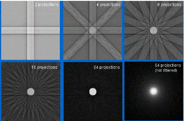
Figure 2.6 - Illustration of back-projection resulting images, with different numbers of projections (Platten, 2003)

By taking the following equation into account:

𝑟 = 𝑥 cos ∅ + 𝑦 sin ∅, (Equation 2.3) The value of each voxel in the resulting image can be defined as:

𝑓′(𝑥, 𝑦) = 1

𝑁∑ 𝑝(𝑥 cos ∅𝑖+ 𝑦 sin ∅𝑖, ∅𝑖) 𝑁

𝑖=1 , (Equation 2.4)

where 𝑓’(𝑥, 𝑦) is the approximation to the true distribution 𝑓(𝑥, 𝑦), 𝑁 is the number of profiles measured and ∅𝑖 is the 𝑖𝑡ℎ projection angle (Cherry et al. 2003).

One of the disadvantages of this technique is the fact that an appreciable amount of blurring occurs due to the presence of projection information outside of the original location on the imaging object. This can be seen in Fig. 6. The process to improve image quality requires the usage of an additional amount of projections in order to reconstruct the image. However, the images will always inherently possess a certain amount of blur, even if an infinite number of projections is taken (Cherry et al. 2003).

2.1.3.1.2. Filtered Back-Projection

In order to fully grasp the concept of filtered back projection (FBP), the notion of Fourier Transforms (FTs) needs to be introduced.

FT allows the representation of a spatially varying function 𝑓(𝑥) in image space as a sum of sine and cosine functions of distinct spatial frequencies 𝑘 in “spatial frequency space”, also known as

(31)

13 | P a g e 𝐹(𝑘) = Ғ[𝑓(𝑥)], (Equation 2.5)

The original 𝑓(𝑥) function can be recovered by applying the inverse FT, which can be represented as:

Ғ−1_{[𝐹(𝑘)] = 𝑓(𝑥),} _{(Equation 2.6)}

This conceptualisation of a FT in one dimension can be further applied to bi-dimensional spaces, such as the projection space 𝑝(𝑟, ∅), by using the projection slice theorem, which states:

Ғ[𝑝(𝑟, ∅)] = 𝑃(𝑘𝑟, ∅), (Equation 2.7)

where 𝑃(𝑘𝑟, ∅) is the value of the FT at a radial distance 𝑘𝑟 along a line at an angle ∅ in k-space

(Cherry et al. 2003).

Using these concepts in an image reconstruction routine, the first step is to measure the projection profiles 𝑝(𝑘𝑟, ∅), at the 𝑁 projection angles, and apply the FT to each projection profile

(Equation 2.7). The next step involves the application of a ramp filter to the resulting 𝑃(𝑘𝑟, ∅),

which means that each projection is to be multiplied by |𝑘𝑟| (Cherry et al. 2003):

𝑃′(𝑘_𝑟, ∅) = |𝑘𝑟|P(𝑘𝑟, ∅) , (Equation 2.8)

Following the application of the ramp filter, the inverse FT for each projection profile is then calculated:

𝑝′(𝑘_𝑟, ∅) = Ғ−1[𝑃′_(𝑘

𝑟, ∅)] = Ғ−1[|𝑘𝑟|P(𝑘𝑟, ∅)], (Equation 2.9)

As a final step, the image can be reconstructed using the filtered projection 𝑝′(𝑟, ∅) and Equation

2.4:

𝑓(𝑥, 𝑦) = 1

𝑁∑ 𝑝′(𝑥 cos ∅𝑖+ 𝑦 sin ∅𝑖, ∅𝑖) 𝑁

𝑖=1 , (Equation 2.10)

where 𝑓(𝑥, 𝑦) is the discretized true distribution. As opposite to the case of a simple back-projection, FBP allows for the reconstruction of the exact true discretized distribution. However, this behaviour is only projected to occur under this formulation in theory, since measured data contains noise, which incurs in a certain degree of image quality degradation that cannot be fully compensated for (Cherry et al. 2003).

Given the speed and relative ease of implementation associated with this reconstruction approach, the FBP can be viewed as one of the most popular reconstruction methods. However, a number of limitations are associated with this reconstruction technique: 1) Data sets containing low count statistics incur in streak artefacts (Cherry et al. 2003); 2) FBP cannot be adjusted in order to consider various characteristics of the PET system, such as the limited spatial resolution associated with the detectors, scattered events, etc. In order to implement these steps extra processing stages are necessary (Cherry et al. 2003).

2.1.3.2. Iterative Reconstruction Methods

These algorithms require more computational power than the analytical methods. However, improvements in their processing speed have led to the implementation of these routines in clinical PET reconstruction. The concept behind these algorithms is illustrated in Fig. 2.7.

(32)

14 | P a g e

Figure 2.7 - Iterative Reconstruction Process (Cherry et al. 2003)

The diagram shown in Fig. 2.7 describes an algorithm that aims to reach the true image distribution 𝑓(𝑥, 𝑦) through a succession of estimates 𝑓 ∗ (𝑥, 𝑦). The first estimate is generally taken as either a uniform intensity or blank image. This initial estimate is then submitted through a process known as forward projection, leading to the generation of a detector response from the imaging object. Associated with this process is the sum of all intensities along the ray paths for all LORs (Cherry et al. 2003).

The calculated projection data 𝑝∗(𝑟, ∅) is compared against the measured data 𝑝(𝑟, ∅). The error in the projected space is then back-projected into the image space and used to provide with an updated estimate of the 𝑓∗(𝑥, 𝑦). This procedure is then repeated in an iterative manner in order to improve the image estimate.

The specifics of the iterative reconstruction methods determine the reasons for these algorithms to incur in a more significant computational load. One reason is that iterative approaches require, logically, that the algorithm runs through a successive number of repetitions towards convergence, until it reaches an acceptable result. Each of these iteration steps include a forward projection and a back projection stages, each one roughly consuming the same amount of time. Since in FBP the back projection step is the most time consuming stage of the algorithm, it is quite understandable that the characteristic nature of iterative methods, which leads to the repetition of this and the forward projection steps for a plurality of times, makes iterative reconstruction algorithms substantially slower in comparison to analytical methods, and FBP in particular. (Cherry et al. 2003)

Iterative algorithms can be viewed as having two essential components: a) the methodology used to compare the measured and current image estimates, in the projection space, 𝑝(𝑥, 𝑦) and 𝑝∗(𝑥, 𝑦); and b) the method that leads to the update of the estimate, 𝑓∗(𝑥, 𝑦), in each iteration. The comparison step is performed with the aid of the cost function and the update of the estimate is done using the update function. This is the general formulation of an iterative reconstruction algorithm, and the development of new methods is basically focused on the usage of new cost or update functions (Cherry et al. 2003).

(33)

15 | P a g e

2.1.3.2.1. Maximum Likelihood Expectation Maximization

(MLEM)

The MLEM algorithm is based on the estimation of the most likely count distribution considering statistical considerations (Cherry et al. 2003), (Matela, 2008).

The acquired data shall be represented by the vector 𝒑, where 𝑝𝑗 is the number of counts in the

𝑗𝑡ℎ_{projection element. A relationship can be established between this measured data and the}

activity in each voxel, using:

𝑝𝑗 = ∑ 𝑀𝑖 𝑖,𝑗𝑓𝑖, (Equation 2.11)

where 𝑓𝑖 is the number of photon pairs produced in voxel 𝑖 and 𝑀𝑖,𝑗 is the system matrix, giving

the probability that the photon pair originating from the 𝑖𝑡ℎ_{voxel is detected in the 𝑗}𝑡ℎ_projection

element (Matela, 2008).

Taking into account Equation 11 and its Poisson statistical nature, as well as the maximum likelihood definition, the following relation can be deduced:

𝑓_𝑖𝑘+1 = 𝑓𝑖𝑘

∑ 𝑀_𝑗 _𝑖,𝑗× ∑ 𝑀𝑖 𝑖,𝑗 𝑝𝑗

∑ 𝑀_𝑣,𝑗𝑓_𝑣𝑘

𝑣 , (Equation 2.12)

where 𝑘 is the iteration number and 𝑓_𝑖𝑘+1 is the activity in each pixel 𝑖 in the next iteration. The elements present in the Equation 12 are intrinsically related to the diagram in Fig. 2.7. The sum element ∑𝑣𝑀𝑣,𝑗𝑓𝑣𝑘 corresponds to the forward projection, which comprises the step when

the information in image space is converted to the projection space (Equation 2.11). The measured data 𝑝𝑗 is afterwards compared to the estimated data by calculating the quotient. This

quotient is weighted by the system matrix element 𝑀𝑖,𝑗 and then summed, which gives the update

factor for each voxel 𝑖. The last step comprises the multiplication of the update factors with the current estimation (divided by the sensitivity in the image space ∑𝑗𝑀𝑖,𝑗), which leads to the

obtainment of an updated image estimation (Matela, 2008).

The MLEM method provides with a good estimate of the real count distribution. However, this approach is associated with two major issues: a significantly high computation time (in comparison with analytic methods, and FBP in particular) – (Kastis et al. 2010) - and stability related issues. These latter issues are related to the fact that the algorithm is based on the attempt to find the signal intensity distribution that best fits the measured data. However, the natural presence of noise in the data leads to the convergence of the algorithm to a solution containing noise as well. In order to avoid the occurrence of too noisy solutions an alternative is to stop the algorithm before the image reaches significantly noisy levels. However, this leads to the obtainment of an image with a particularly limited spatial resolution (Matela, 2008). This noise/spatial resolution relationship is the main compromise that needs to be taken into account in iterative reconstruction algorithms, although this relationship is also true for FBP.

Additional information regarding the derivation of Equation 12 can be found in Matela (2008).

Myocardial partial volume correction of internal left ventricular structures in emission tomography images

FACULDADE DE CIÊNCIAS

DEPARTAMENTO DE FÍSICA

Myocardial partial volume correction of internal left

ventricular structures in emission tomography images

Mauro Santana Costa e Sousa

Dr. Kris Thielemans, Institute of Nuclear Medicine, University College London,

London, UK

Prof Dr. Pedro Almeida, Instituto de Biofísica e Engenharia Biomédica, Departamento

de Física da Faculdade de Ciências da Universidade de Lisboa, Lisboa, Portugal

MESTRADO INTEGRADO EM ENGENHARIA BIOMÉDICA E BIOFÍSICA

PERFIL: RADIAÇÕES EM DIAGNÓSTICO E TERAPIA

FACULDADE DE CIÊNCIAS

DEPARTAMENTO DE FÍSICA

Myocardial partial volume correction of internal left

ventricular structures in emission tomography images

Mauro Santana Costa e Sousa

Dissertação Orientada por Doutor Kris Thielemans e Professor Doutor

Pedro Almeida

Mestrado Integrado em Engenharia Biomédica e Biofísica

Perfil em Radiações em Diagnóstico e Terapia

Acknowledgements

Resumo

Abstract

Contents

ACKNOWLEDGEMENTS

I

RESUMO

II

ABSTRACT

V

TABLE OF FIGURES

IX

LIST OF TABLES

XII

LIST OF ABBREVIATIONS

XIII

INTRODUCTION

1

BACKGROUND

4

PVC METHODS

21

METHODS

31

RESULTS AND DISCUSSION

39

SUMMARY, CONCLUSIONS AND FUTURE PROSPECTS

88

PUBLICATIONS

90

Table of Figures

List of Tables

List of Abbreviations

Introduction

1.1. Project Framework

1.2. Motivation

1.2.1. Layout of the Report

Background

2.1. Positron Emission Tomography

2.1.1.

Basic PET Principles

2.1.2. Data Correction

2.1.2.1. Attenuation Correction

2.1.2.2. Scatter Correction

2.1.2.3. Correction of Random Events

2.1.2.4. Partial Volume Effect and Partial Volume Correction

2.1.3. PET Image Reconstruction

2.1.3.1. Analytical Reconstruction Methods

2.1.3.1.1.

Simple Back-projection

2.1.3.1.2.

Filtered Back-Projection

2.1.3.2. Iterative Reconstruction Methods

2.1.3.2.1.

Maximum Likelihood Expectation Maximization

(MLEM)