Misfortunes never come singly

(1)

1

Misfortunes Never Come Singly:

Consecutive Weather Shocks and Mortality in Russia

(Published in Economics and Human Biology 31, 2018)

https://doi.org/10.1016/j.ehb.2018.08.008

Vladimir Otrachshenko a,b

a_{Nova School of Business and Economics, Campus de Campolide, 1099-032 Lisbon, Portugal. E-mail:} vladotr@novasbe.pt

b _{Leibniz Institute for East and Southeast European Studies (IOS), Landshuter Str. 4, 93047} Regensburg, Germany

Olga Popova * b,c,d *Corresponding author

b_{Leibniz Institute for East and Southeast European Studies (IOS), Landshuter Str. 4, 93047} Regensburg, Germany.

E-mail: popova@ios-regensburg.de

c _{CERGE-EI, a joint workplace of Charles University and the Economics Institute of the Czech Academy} of Sciences, Politickych veznu 7, 111 21 Prague, Czech Republic

d _{Graduate School of Economics and Management, Ural Federal University, Mira 19, 620002} Yekaterinburg, Russian Federation

Pavel Solomin e

e_{Instituto Superior de Engenharia de Lisboa (ISEL), Rua Conselheiro Emídio Navarro 1, 1959-007} Lisbon, Portugal E-mail: p.o.solomin@gmail.com

Acknowledgements

Olga Popova acknowledges the support from the Russian Science Foundation (RSF) Grant No. 15-18-10014 "Projection of optimal socio-economic systems in turbulence of external and internal environment". Vladimir Otrachshenko acknowledges the research fellowship from Fundação para a Ciência e a Tecnologia, Portugal (SFRH/BPD/122946/2016). All opinions expressed are those of the authors and have not been endorsed neither by the RSF, nor by the FCT. Vladimir Otrachshenko acknowledges the hospitality of the Leibniz Institute for East and Southeast European Studies (IOS), Regensburg, Germany, where the part of this paper was developed. The authors thank five anonymous referees and participants at seminars and workshops in Bayreuth, Lisbon, Regensburg, Passau, Vladivostok, and Yekaterinburg for useful comments and suggestions.

(2)

2

Misfortunes Never Come Singly:

Consecutive Weather Shocks and Mortality in Russia

Abstract

This paper examines the impacts of extremely hot and cold days on mortality in Russia, using a 25-year regional panel data. Unlike other studies, the sequence of those extreme days is also taken into account, that is, the impacts of both single and consecutive (i.e. heat waves and cold spells) extreme days are estimated simultaneously. We demonstrate the importance of accounting for the sequence of extreme days. We also disentangle the impacts of those extremes by age and gender. The findings suggest that single hot days increase mortality, while single cold days do not affect mortality. On the other hand, both consecutive hot and consecutive cold days increase mortality in females and males for all age groups, although males are affected more severely. Overall, consecutive days with extreme temperatures impose considerable costs to society in terms of years of life lost. Thus, ignoring the sequences of extreme days that are likely to increase in the future because of climate change may have critical implications for mitigation policies.

Keywords: Climate Change; Cold Spells; Extreme Weather; Heat Waves; Mortality; Russia JEL Codes: I14; J16; J17; Q54

(3)

3 1. Introduction

The empirical link between extreme weather events and mortality is well documented in epidemiology and social sciences (Basu and Samet, 2002; Dell et al., 2014; Deschenes, 2014). Epidemiological literature mostly examines the impact of heat waves and cold spells, i.e. consecutive hot and cold days, on mortality, using evidence from location-specific case studies (Basu, 2009; Basu and Samet, 2002; Gosling et al., 2009). In contrast, existing studies in social sciences such as economics, analyze a single-day impact of a specific cold or hot temperature on mortality, using countrywide regional panel data (Dell et al., 2014). To date, evidence from countrywide regional panel data regarding the impact of one additional day with a specific cold or hot temperature on mortality exists for the U.S., India, Mexico, and Russia.1_{Those studies} assume that the impacts of single and consecutive days are the same.

As stated by Intergovernmental Panel on Climate Change (IPCC, 2014), the frequency of heat waves and cold spells will increase in the future because of climate change.This paper disentangles the impacts of single and consecutive cold/hot days on individuals’ mortality and presents evidence that the impacts of those days may impose different costs to society.Thus, ignoring consecutive days that are likely to increase in the future may have critical implications for mitigation policies.

According to epidemiological case studies, heat waves and cold spells contribute to excess mortality. However, there is no consensus regarding the magnitude of an impact of those waves. The estimated impacts vary substantially across studies that can be explained by several reasons.2

1_{See Barreca (2012), Barreca et al. (2015) and (2016), Deschênes and Moretti (2009), Deschênes and Greenestone}

(2011) for evidence on the U.S., Burgess et al. (2017) for India, Cohen and Dechezlepretre (2017) for Mexico, and Otrachshenko et al. (2017) and Portnykh (2017) for Russia.

2_{The estimated increase in the daily number of deaths during heat waves is 0.2% based on data from several U.S.} cities (Gasparrini and Armstrong, 2011); 12.1% in the Netherlands (Huynen et al., 2001); 5.5% in London, 9.3% in Budapest, and 15.2% in Milan (Hajat et al., 2006); 33% in Moscow (Revich and Shaposhnikov, 2012); 60% in France (Poumadère et al., 2005); and 85% in Chicago (McGeehin and Mirabelli, 2001). The impact of cold spells is estimated to be 1.83% in Sofia (Pattenden et al., 2003), 8.9% in Moscow (Revich and Shaposhnikov, 2012), and 12.8% in the Netherlands (Huynen et al., 2001).

(4)

4 First, epidemiological and medical studies vary substantially in the study design quality. The findings are typically location-specific and based on data from a single location or on a small number of locations for a limited time period. Also, epidemiological studies typically analyze not the direct impact of extreme temperature on mortality, but compare the mortality during the heat wave with the mortality in a baseline period of non-extreme temperature days (Deschênes and Greenstone, 2011). Finally, there are also differences in the definition of heat waves and cold spells between studies. For instance, Huynen et al. (2001) define heat wave as a “period of at least 5 days, each of which has a maximum temperature of at least 25°C, including at least 3 days with a maximum temperature of at least 30°C” (p. 463), while “a cold spell is a period of at least 9 days with a minimum temperature of -5°C or lower, of which at least 6 days have a minimum temperature of -10°C or lower” (p. 464).Hajat et al. (2006) define heat wave as a period of two or more days at temperatures above the 99th_{percentile daily mean temperature, while Gasparrini} and Armstrong (2011) suggest that heat wave as a period of at least two days at temperatures above the 97th_{percentile median daily temperature.}

Moreover, most epidemiological studies use either daily or monthly data on mortality, and thus, those studies account only for a short-run impact of heat waves and cold spells on mortality, may overestimate the impact of temperature due to short-run mortality displacements, and cannot estimate the overall impact in terms of the total annual number of deaths (Deschênes and Greenstone, 2011). In this paper we address those limitations by using the annual countrywide regional panel data.

In this study we define consecutive days, both cold and hot, as at least three days with a specific temperature range that follow in a sequence. Unlike other studies, we estimate the impacts of single and consecutive days simultaneously. Using a novel 25-year regional panel data on Russia, this paper examines the causal impacts of single and consecutive cold and hot days on the all-cause annual regional mortality. We also quantify a social impact in terms of year of life lost due to extremely hot and cold temperatures.

(5)

5 We also distinguish the impacts between gender and age groups and study the adaptation to extreme weather days.

The rest of the paper is organized as follows. The next section reviews the literature and summarizes the channels that explain the impact of weather on mortality. Then, the methodology and data sections are presented. We then present the estimation results related to weather shocks, compute their social impact, discuss the adaptation of warm and cold regions to weather extremes, and present the robustness checks. The final section offers conclusions and discusses the avenues for future research.

2. Literature Review

Excess mortality due to weather shocks is primarily explained by hypothermia and hyperthermia (Basu and Samet, 2002). According to epidemiological literature, the most comfortable winter temperature for human well-being is between 68°F and 74°F (20-23.3°C) and the summer temperature is between 73°F and 78°F (22.3-25.6°C) (Burroughs and Hansen, 2011). Ambient air temperatures exceeding comfortable limits are treated by the human body as a thermal stress and induce physiological adjustment and thermoregulation by changes in blood pressure, viscosity, heart rate, bronchoconstriction, shivering, and cellular and humoral immunity (Basu and Samet, 2002; Martens, 1998). This increases the likelihood of cardiovascular and respiratory systems diseases and leads to greater death risks.3

Previous economic studies examine a one-day impact of extremely hot and cold temperature on mortality.4_{For instance, Deschênes and Greenstone (2011) suggest that a hot day (with average} temperature above 90°F, i.e. 32.2°C) increases annual mortality by 0.11%, while a cold day (below 20°F, i.e. -6°C) increases annual mortality by 0.08% in the U.S. Burgess et al. (2017) suggest that the impact of

3_{Recent evidence suggests that in utero exposure to temperature variability is also detrimental to health (Molina}

and Saldarriaga, 2017).

4_{It should be noted that due to methodological differences (e.g., frequency of data used, use of temperature bins} or temperature itself, and/or use of different baseline temperature bins), the findings from different economic studies may not be directly comparable.

(6)

6 a single hot day in India is higher than in the U.S. The authors find that a day with mean temperature above 95°F (35°C) increases annual mortality by 0.74%. A cold day (below 65°F, i.e. 18.3°C) has no statistically significant effect on mortality in India.

Recently, Otrachshenko et al. (2017) find that in Russia, a day above 25°C increases all-cause mortality by 0.06%, while a cold day with a temperature range between −30°C and−25°C increases mortality by 0.08%. The authors also suggest that population in regions with frequent hot temperatures adapts to such extreme. Also, population in cold regions adapts to extremely cold temperature. This conclusion is supported by Portnykh (2017).

Using data from Mexico, Cohen and Dechezlepretre (Cohen and Dechezleprêtre, 2017) also suggest that cold days are more harmful than hot days. The authors find that an extremely hot day (above 32°C) increases annual mortality by 0.03%, while a cold day (below 10°C) increases annual mortality by 0.15%. The literature also documents a phenomenon defined as mortality displacement or “harvesting” (Basu and Samet, 2002; Deschênes and Moretti, 2009). This effect implies an increasing likelihood of death during days with extreme temperature for elderly and people with diseases, that is, people with a higher risk of death as compared to the general population. Such effect may explain up to 50% of the estimated increase in mortality during heat waves (Revich and Shaposhnikov, 2012).5_{Since days with extreme} temperature select out individuals with a higher risk of death, leaving individuals with a lower risk of death alive, the harvesting effect also implies that mortality during subsequent days with moderate temperature is lower. Thus, there is no long-run impact of harvesting on mortality, since an increase in mortality in a short-run is offset by lower mortality during days with subsequent moderate temperature (Deschênes and Greenstone, 2011; Deschênes and Moretti, 2009).

5_{The stress-related harvesting effect may also explain the elevated risk of death among the elderly and the}

individuals personally affected by events not related to weather such as, for instance, the Great Recession (Crost and Friedson, 2017; Falconi et al., 2016). However, social, behavioral, and biological changes during the economic downturn may be too short-lived to affect the mortality of other groups of population (Ásgeirsdóttir et al., 2016).

(7)

7 Since the sign of the short-run harvesting effect varies between days with extreme and moderate temperature, it is difficult to fully eliminate this effect in the estimation if daily or monthly data on mortality are used (Deschênes and Greenstone, 2011). In this paper we use the annual mortality data for estimating the impact of heat waves and cold spells. The use of annual data helps to avoid dealing with harvesting, since data are sufficiently aggregated to capture the short-run differences in mortality between days with extreme and moderate temperature. As suggested by Deschênes and Greenstone (2011), “the combination of annual mortality data and aggregated daily temperature data should be sufficient to flexibly capture the full dynamic relationship between temperature and mortality” (p. 173).

3. Methodology

To estimate the relationship between mortality and temperature, we follow Deschênes and Greenstone (2011), Burgess et al. (2017), and Otrachshenko et al. (2017). The model is estimated separately for men and women.

= + + !"

# $ "

% & +

+Ө(_{) *} _∗ _{, + - + . + (1)}

where the subscripts i and t stand for a region and year, respectively. is the annualmortality rate per 1,000,000 inhabitants. is the number of days in a region i and year t in which the mean daily temperature fell in the j-th of the 18 bins. The temperature bin (19°C, 22°C] is omitted and used as a default bin. Each temperature bin is interpreted as the impact of one-day in a specific temperature range on the annual mortality rate compared to the default bin. is the number of days in spells of at least three consecutive days with extremely cold (below -23°C) or extremely hot (above 25°C) temperature. Each consecutive bin is interpreted as the impact of each day in a spell of at least three consecutive days with extreme temperature compared to the default bin (19°C, 22°C].

(8)

8 % & is the number of days in a region i and year t in which the mean daily precipitation fell in the

n-th of the 3 bins. The precipitation bin [0 mm, 10 mm) is omitted and used as a default bin. The definition

of temperature and precipitation bins is discussed in the next section.

It might be the case that the trends in health and economic outcomes in certain regions correlate with climate change. Thus, to control for this geographical difference over the period studied, we introduce the region-specific trends, ) * ∗ ,, where ) * is a set of dummy variables and equals one for a region i and 0 otherwise, while Trend is a linear time trend.

- and . are the regional and time fixed effects, respectively. The regional fixed effects control for time invariant unobserved regional characteristics that may affect mortality, while the time fixed effects control for any common changes across regions (i.e. health sector reforms). is an error term.

The standard errors in Eq. (1) are clustered at the regional level. We also weight all regressions by the relevant regional population. Eq. (1) is estimated separately for men and women of several age groups, including all-age, 20-29, 30-39, 40-49, 50-59, 60-69, and above 70 years old.

4. Data

In this study we use data on 79 regions of Russia from 1989 to 2014.6_{Data on mortality are average}

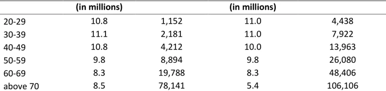
annual mortality rates per 1,000,000 inhabitants in a given region by gender and age groups from the Federal Statistical Service of the Russian Federation. The average population and mortality rates by gender and age groups are in Table 1.

Table 1: Average population and average annual mortality rates from 1989 to 2014

Age Groups: Female Male

Population Mortality Rate Population Mortality Rate

6_{According to the Constitution of the Russian Federation, the number of regions in Russia is 83 in 2013. Due to the}

(9)

9

(in millions) (in millions)

20-29 10.8 1,152 11.0 4,438 30-39 11.1 2,181 11.0 7,922 40-49 10.8 4,212 10.0 13,963 50-59 9.8 8,894 9.8 26,080 60-69 8.3 19,788 8.3 48,406 above 70 8.5 78,141 5.4 106,106

Source: Authors’ computations based on the data from the Federal Statistical Service of the Russian Federation. Notes: Mortality rates are per 1,000,000 of population of particular gender and age group.

The temperature and precipitation data are collected from 518 ground stations. To aggregate the ground station data to the level of regions, we first weight data from each ground station based on the inverse distance square to the closest settlement within the radius of 200 km in each region.Then, each settlement is given a weight based on its population.This methodology is suggested by Hanigan et al. (2006), and helps to receive the average weather experienced by a person in a given region.7

The coldest month in Russia is January, with the mean monthly temperature -25.2°C, and the warmest month is July, with 15.1°C.8_{Figure 1 shows the frequency of days in a particular temperature} range during the 1989-2014 period.

Figure 1: Frequency of days with a particular temperature range

Source: Authors’ construction

7_{For a discussion of different weighting approaches, see also Dell et al. (2014).} 8_{See World Bank (2016).}

0 0.02 0.04 0.06 0.08 0.1 -2 3 °C a n d b el o w -2 3 °C -20 °C -2 0 °C -17 °C -1 7 °C -14 °C -1 4 °C -11 °C -1 1 °C -8 °C -8 °C -5 °C -5 °C -2 °C -2 °C 1 °C 1° C 4 °C 4° C 7 °C 7 °C 1 0 °C 1 0 °C 1 3 °C 1 3 °C 1 6 °C 1 6 °C 1 9 °C 1 9 °C 2 2 °C 2 2 °C 2 5 °C 2 5 °C 2 8 °C ab o ve 2 8 °C

(10)

10 As shown in this figure, days with the average daily temperature above 28°C are still rare in the Russian regions. Thus, we merge the bins with the 25-28°C and above 28°C. Thus, the hottest temperature bin in our model is the number of days with mean daily temperature above 25°C. Similarly, even though some regions have experienced the temperatures from -60°C to -23°C, we merge all coldest temperatures into one bin below -23°C. Thus, we use 18 temperature bins that include a number of days in a particular temperature range in a given region and year: (below -23°C], (-23°C, -20°C], (-20°C, -17°C], (-17°C, -14°C], (-14°C, -11°C], (-11°C, -8°C], (-8°C, -5°C], (-5°C, -2°C], (-2°C, 1°C], (1°C, 4°C], (4°C, 7°C], (7°C, 10°C], (10°C, 13°C], (13°C, 16°C], (16°C, 19°C], (19°C, 22°C], (22°C, 25°C], and (above 25°C). The default bin is with the 19-22°C temperature range, which is considered as a comfortable temperature for the human body.

Apart from bins with single days in a particular temperature range, we also construct two bins with consecutive extremely cold or hot days. Those bins include the number of days in spells of at least three consecutive days with extremely cold (-23°C and below) or extremely hot (above 25°C) mean daily temperature. 81% of regions in our sample have experienced such consecutive cold days, and 85% of regions have experienced consecutive hot days. On average, there are 7.51 cold and 3.95 hot consecutive days in Russia during the period studied. The annual number of days in our analysis is standardized to 365. We also construct three bins related to the precipitation level: [0mm, 10mm), [10mm, 20mm), and [above 20mm).

5. Estimation Results

We start by examining the impacts of single and consecutive days with a particular temperature on all-cause mortality in men and women.9_{Then we present the estimation results related to the impact of} extremely hot (above 25°C) and extremely cold (below -23°C) temperatures on mortality by age and gender groups. Next, we compute the years of life lost due to extremely hot and extremely cold days, both single

(11)

11 and consecutive. Finally, we discuss adaptation to those events in warm and cold regions and present the robustness checks.

The results discussed in this section represent the impact on total mortality rate per 1,000,000 inhabitants of each gender.10_{The default temperature bin is between 19°C and 22°C, for precipitation is} between 0mm and 10mm, and for consecutive days is one or two days with a particular temperature range. Table 2 presents the estimation results for the impacts of both single and consecutive days with a particular temperature on the total all-age mortality. In this table, models (1a) and (1b) present the estimation results for females and males when using the temperature bins with the single days, ignoring their sequence. Models (2a) and (2b) present the estimation results for females and males when the sequence of days with extremely hot and cold temperatures is taken into account. As shown in models (1a) and (1b), we find that a single day with temperature above 25°C increases the mortality in both females and males, and the impact is greater for males: 12.32 deaths per 1,000,000 females vs. 20.86 deaths per 1,000,000 males, when compared to a single day with a temperature between 19-22°C. Similarly, a single cold day with temperature below -23°C also increases the female mortality rate by 16.06 and the male mortality by 25.51.

As shown in models (2a) and (2b), the impact of consecutive hot days is also considerable. Interestingly, when single and consecutive cold days are disentangled, a single day with temperature below -23°C does not affect neither female, nor male mortality, while each day in a spell of at least three consecutive days with the same temperature increases the female mortality rate by 15.57 and the male mortality rate by 20.20. We also test the differences between the impacts of the consecutive cold day bin

and single cold day bins. We find the difference between the impact of the consecutive cold day bin and

the impact of (below -23°C], (-23°C,20°C], (-11°C, -8°C], and (-2°C, 1°C] single day bins for females, and of (below -23°C], (-23°C,20°C], and (-11°C, -8°C] for males.

(12)

12 These results underscore that the importance of taking consecutive days into account and that mortality in both women and men increases during cold spells, not during single extremely cold days. Such impact can be explained by behavioral adjustment to cold temperature. In the case of a single cold day, individuals may stay indoors to protect themselves from cold without any harm for their regular activities, e.g. job, while in the case of a cold spell, they might be forced to go outside to perform regular activities. Regarding the impact of days with temperature above 25°C, we find the impacts of both single and consecutive days for both females and males (see models 2a and 2b in Table 2).

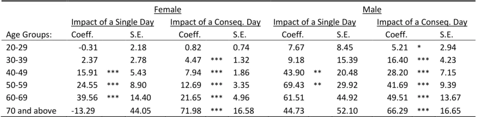
Each age group may have different likelihood of death due to weather extremes. Therefore, we next discuss the results by gender and age groups. The results for the combined model of single and consecutive day bins for extremely hot and extremely cold temperatures are in Tables 3 and 4, respectively.

As shown in Table 3, consecutive days with temperature above 25°C increase mortality in both females and males of all age groups, except for the 20-29 years old females, while single days with the same temperature affect only some groups of population (the 40-49, 50-59, and 60-69 years old females and the 40-49 and 50-59 years old males). This result suggests that a single hot day may not necessarily be harmful, while consecutive days (heat waves) are indeed harmful and increase mortality of all age and gender groups.

Regarding the impact of cold days, we find that a single day with temperature below -23°C does not affect any age and gender group, while consecutive cold days are harmful, especially for older groups of population, in particular, above 70 years old females and above 40 years old males (see Table 4).

(13)

13

Table 2: The impacts of single and consecutive days with a specific temperature on the total all-age mortality

Model: (1a) (1b) (2a) (2b)

Dependent Variable: Female Male Female Male

Mortality Coeff. S.E. Coeff. S.E. Coeff. S.E. Coeff. S.E.

Conseq.(below -23°C] - - 15.57 *** 2.85 20.20 *** 5.49 (below -23°C] 16.06 *** 3.16 25.51 *** 6.78 -3.84 4.80 -3.85 9.11 (-23°C, -20°C] 6.03 4.54 -6.08 9.07 7.78 * 4.37 -5.67 9.25 (-20°C, -17°C] 13.44 ** 3.35 14.37 ** 6.80 12.20 *** 3.56 10.38 6.84 (-17°C, -14°C] 15.53 *** 3.03 20.41 *** 6.83 13.80 *** 2.93 15.57 ** 6.17 (-14°C, -11°C] 12.35 3.84 12.88 8.42 10.78 ** 3.85 8.38 7.98 (-11°C, -8°C] 10.40 ** 2.81 14.05 ** 5.23 8.84 *** 2.58 10.07 * 5.06 (-8°C, -5°C] 12.82 *** 3.09 17.97 *** 5.86 11.26 *** 3.32 14.11 ** 6.04 (-5°C, -2°C] 12.27 ** 3.20 15.29 ** 6.50 10.88 *** 3.08 11.61 * 6.19 (-2°C, 1°C] 9.53 *** 2.10 17.88 *** 5.46 8.58 *** 2.22 14.97 ** 5.80 (1°C, 4°C] 4.29 2.87 4.56 5.00 3.18 3.08 1.59 5.33 (4°C, 7°C] 5.38 2.57 7.38 5.08 4.13 2.51 4.36 4.91 (7°C, 10°C] 9.47 *** 2.11 16.54 *** 4.06 8.74 *** 2.15 14.41 *** 4.15 (10°C, 13°C] 3.50 ** 1.54 7.86 ** 3.16 2.98 * 1.58 6.22 * 3.15 (13°C, 16°C] 5.07 * 1.96 8.76 * 4.49 4.73 ** 2.07 7.73 4.70 (16°C, 19°C] 2.87 * 1.90 8.41 6.34 2.18 2.03 6.73 6.57 (22°C, 25°C] 7.27 ** 2.45 16.00 ** 6.37 6.99 ** 2.75 15.18 * 6.80 (above 25°C] 12.32 *** 2.68 20.86 *** 4.85 13.70 ** 6.09 24.77 * 15.01 Conseq.(above 25°C] - - 10.49 *** 2.91 17.29 *** 5.00 [10mm, 20mm) -0.26 4.82 -9.43 8.49 -0.39 4.83 -9.28 8.61 [above 20mm) 10.83 9.61 24.34 24.17 10.88 9.63 24.61 24.03

Regional Fixed Effects Yes Yes Yes Yes

Time Fixed Effects Yes Yes Yes Yes

Regional Linear Trends Yes Yes Yes Yes

R2

within 0.89 0.88 0.89 0.88

Nr. Of Obs. 2,047 2,047 2,047 2,047

Notes: Models 1a and 1b present the results with single day effects for females and males, respectively. Models 2a and 2b present the results of the

combined specification that includes both single and consecutive day effects for females and males, respectively. Robust standard errors are clustered at a regional level. The regional population weights are applied. The temperature bin (19°C, 22°C] and the precipitation bin [0 mm, 10 mm) are used as a default. ***, **, * stand for 1%, 5%, and 10% significance levels, respectively.

(14)

14

Table 3: The impacts of single and consecutive days with temperature above 25°C on mortality by age groups

Female Male

Impact of a Single Day Impact of a Conseq. Day Impact of a Single Day Impact of a Conseq. Day

Age Groups: Coeff. S.E. Coeff. S.E. Coeff. S.E. Coeff. S.E.

20-29 -0.31 2.18 0.82 0.74 7.67 8.45 5.21 * 2.94 30-39 2.37 2.78 4.47 *** 1.32 9.18 15.39 16.40 *** 4.23 40-49 15.91 *** 5.43 7.94 *** 1.86 43.90 ** 20.48 28.20 *** 7.15 50-59 24.55 *** 8.90 12.69 *** 3.35 69.43 ** 29.92 41.69 *** 9.39 60-69 39.56 *** 14.40 21.65 *** 4.96 61.51 44.92 49.51 *** 13.67 70 and above -13.29 44.05 71.98 *** 16.58 44.73 52.10 66.29 *** 16.65

Notes: The results from the combined model of single and consecutive day effects are presented. Robust standard errors are clustered at a

regional level. The regional population weights of a particular age group are applied. The temperature bin (19°C, 22°C] and the precipitation bin [0 mm, 10 mm) are used as a default. The impact of a single day corresponds to an impact of a single day with temperature above 25°C, while the impact of a consecutive day corresponds to an impact of each day in a sequence of at least three days with temperature above 25°C. ***, **, * stand for 1%, 5%, and 10% significance levels, respectively.

Table 4: The impacts of single and consecutive days with temperature below -23°C on mortality by age groups

Female Male

Impact of a Single Day Impact of a Conseq. Day Impact of a Single Day Impact of a Conseq. Day

Age Groups: Coeff. S.E. Coeff. S.E. Coeff. S.E. Coeff. S.E.

20-29 -0.91 1.61 -0.57 1.06 -2.62 6.16 -5.49 3.39 30-39 -4.82 3.01 2.65 2.20 -13.58 8.33 8.85 5.83 40-49 -6.36 4.85 6.81 3.04 -13.05 12.33 22.21 ** 8.81 50-59 -13.47 8.59 7.82 4.95 0.50 19.36 25.56 ** 11.91 60-69 -7.34 10.96 -0.29 7.62 -40.72 24.87 48.54 ** 19.31 70 and above -31.87 30.89 73.35 *** 18.27 -3.87 40.86 102.73 *** 21.80

Notes: The results from the combined model of single and consecutive day effects are presented. Robust standard errors are clustered at a

regional level. The regional population weights of a particular age group are applied. The temperature bin (19°C, 22°C] and the precipitation bin [0 mm, 10 mm) are used as a default. The impact of a single day corresponds to an impact of a single day with temperature below -23°C, while the impact of a consecutive day corresponds to an impact of each day in a sequence of at least three days with temperature below -23°C. ***, **, * stand for 1%, 5%, and 10% significance levels, respectively.

(15)

15 5.1 Years of Life Lost due to Weather Shocks

To show the social impact of our results, for males and females of each age group, we compute the annual number of deaths and the years of life lost due to extreme temperatures.

Table 5showsthe results for the impacts of single and consecutive days with temperature above 25°C on mortality in males and females. This table is divided in two parts. The first part corresponds to the model that accounts only for the impact of a single day with such temperature range, and the second corresponds to the model that accounts for the impacts of single and consecutive days simultaneously.

In Table 5 we first compute the average annual number of deaths due to one day with temperature above 25°C (see columns (1) and (2) for females and males, respectively). Columns (1) and (2) are computed by multiplying the estimated impacts of a single day and a consecutive day above 25°C by the average regional population of each gender and age group. Columns (3) and (4) present the years of life left (YLL) for each age group, i.e. the number of additional years that an average person would have lived if he/she was not affected by a mortality risk due to extremely hot weather. The YLL are calculated based on the life expectancy of each gender and age group. For each age group, we take the life expectancy of the upper age limit (e.g., to calculate the YLL for a group of 20-29 year olds, we use the life expectancy of 29 year olds for each gender). Columns (5) and (6) show the total number of YLL for females and males, respectively. (5) is computed by multiplying the columns (1) and (3), while (6) is computed by multiplying the columns (2) and (4).

While using the life expectancy data to calculate the YLL, we assume that individuals would have reached the life expectancy age of their age and gender group if an extremely hot/cold day would not occur. However, this approach may overestimate the YLL if the affected individuals are more fragile and have a worse health than the average population, i.e. have a shorter life expectancy than an average person in their age and gender group (Deschenes and Moretti, 2009). This may occur due to the advanced displacement of deaths in a short run (harvesting effects). However, the use of annual data may help to deal with such harvesting effects, as discussed in the literature review section.

(16)

16 Table 5: Estimated number of deaths and years of life lost due to a single and to a consecutive hot day

(1) (2) (3) (4) (5) (6)

Estimated Number of Death Years of Life Lost Total Years of Life Lost

Im p a ct o f a S in g le D a y a b o v e 2 5 °C

Age Groups Female Male Female Male Female Male

20-29 14 70 52.3 41.1 732 2,877 30-39 30 201 43.0 33.0 1,290 6,633 40-49 107 338 33.9 25.3 3,627 8,551 50-59 156 413 25.2 18.1 3,931 7,475 60-69 217 295 17.2 12.3 3,732 3,629 70 and above 405 195 13.4 9.9 5,427 1,931 Total 929 1,512 18,740 31,096 Im p a ct s o f S in g le a n d C o n se cu ti v e D a y s a b o v e 2 5 °C a C o n se cu ti v e D a y a S in g le D a y

20-29 -3a ₈₄a _52.3 _41.1 _-157 _3,452 30-39 26a ₁₀₁a _43.0 _33.0 _1,118 _3,333 40-49 171 438 33.9 25.3 5,797 11,081 50-59 241 558 25.2 18.1 6,073 10,100 60-69 327 330a _17.2 _12.3 _5,624 _4,059 70 and above -79a ₁₁₅a _13.4 _9.9 _-1,059 _1,139 Total 739 996 17,495 21,181

20-29 9a ₅₇ _52.3 _41.1 ₄₇₁ _2,343 30-39 50 180 43.0 33.0 2,150 5,940 40-49 85 282 33.9 25.3 2,882 7,135 50-59 125 335 25.2 18.1 3,150 6,064 60-69 179 265 17.2 12.3 3,079 3,260 70 and above 427 170 13.4 9.9 5,722 1,683 Total 866 1,289 16,982 26,423

Notes:The first part of this table corresponds to the model where the impacts of single and consecutive days are assumed to be the same while the second part corresponds to the model where those impacts are disentangled. a_is

based on a non-significant coefficient. (1) and (2) are computed by multiplying the estimated impact of a single or a consecutive day above 25°Cby the average regional population of each gender and age group. Columns (3) and (4) represent the years of life lost for each gender and age group. Total years of life lost are presented in columns (5) and (6). (5) is computed by multiplying columns (1) and (3), while (6) is computed by multiplying columns (2) and (4). Rows, Total, are computed by summing up the results from significant coefficients.

As shown in the first part of Table 5, in most age groups the annual estimated number of deaths due to days above 25°C is greater for males than for females, except for the elderly. Overall, as shown in columns (5) and (6), the total number of YLL is greater for males when compared to females (18,740 vs. 31,096, respectively).

(17)

17 In the second part of Table 5, the impacts of single and consecutive days are disentangled. As shown, a single day with temperature above 25°C affects the mortality in the 40-49, 50-59, and 60-69 years old females and in the 40-49 and 50-59 years old males. Regarding the impact of one consecutive day, it is harmful for all age categories of both genders, except for young females. Overall, one consecutive hot day increases mortality by 15% in females and by 23% in males when compared to the impact of a single day (for females 739 vs. 866 and for males 996 vs. 1,289, respectively). Thus, consecutive hot days lead to remarkable reductions in the years of life, and the impact is greater for males. It is worth mentioning that for both genders, the impact of a single day is larger in the model when consecutive days are taken into account (for females, 929 vs. 739, and for males, 1,512 and 1,289, respectively).

Table 6 presents the results for the impacts of single and consecutive days with temperature below -23°C on the mortality by gender and age groups and can be interpreted in the same manner as Table 5. As shown in Table 6, the total number of YLL in both models (with and without consecutive days) is greater for males when compared to females. However, there is a remarkable difference between two models. In the second part of Table 6, we observe no impact of a single cold day on the mortality of both genders when the sequence of extremely cold days is taken into account. In fact, we find that only consecutive days matter.

(18)

18 Table 6: Estimated number of deaths and years of life lost due to a single and to a consecutive cold day

(1) (2) (3) (4) (5) (6)

Estimated Number of Death Years of Life Lost Total Years of Life Lost

Im p a ct o f a S in g le D a y b e lo w -2 3 °C

20-29 -8a _-66 _52.3 _41.1 _-418 _-2,713 30-39 29a ₈₇a _43.0 _33.0 _1,247 _2,871 40-49 68a ₂₇₂ _33.9 _25.3 _2,305 _6,882 50-59 29a ₃₁₄ _25.2 _18.1 ₇₃₁ _5,683 60-69 -52a ₁₆₁a _17.2 _12.3 _-894 _1,980 70 and above 307 245 13.4 9.9 4,114 2,426 Total 307 765 4,114 12,278 Im p a ct s o f S in g le a n d C o n se cu ti v e D a y s b e lo w -2 3 °C a C o n se cu ti v e D a y a S in g le D a y

20-29 -10a _-29a _52.3 _41.1 _-523 _-1,192 30-39 -54a _-149a _43.0 _33.0 _-2,322 _-4,917 40-49 -68a _-130a _33.9 _25.3 _-2,305 _-3,289 50-59 -132a ₄a _25.2 _18.1 _-3,326 ₇₂ 60-69 -61a _-218a _17.2 _12.3 _-1,049 _-2,681 70 and above -189a _-10a _13.4 _9.9 _-2,533 _-99 Total 0 0 0 0

20-29 -6a _-60a _52.3 _41.1 _-314 _-2,466 30-39 29a ₉₇a _43.0 _33.0 _1,247 _3,201 40-49 73a ₂₂₂ _33.9 _25.3 _2,475 _5,617 50-59 77a ₂₀₅ _25.2 _18.1 _1,940 _3,711 60-69 -2a ₂₆₀ _17.2 _12.3 _-34 _3,198 70 and above 436 264 13.4 9.9 5,842 2,614 Total 436 951 5,842 15,139

Notes:The first part of this table corresponds to the model where the impacts of single and consecutive days are assumed to be the same while the second part corresponds to the model where those impacts are disentangled. a_is

based on a non-significant coefficient. (1) and (2) are computed by multiplying the estimated impact of a single or a consecutive day below -23°Cby the average regional population of each gender and age group. Columns (3) and (4) represent the years of life lost for each gender and age group. Total years of life lost are presented in columns (5) and (6). (5) is computed by multiplying columns (1) and (3), while (6) is computed by multiplying columns (2) and (4). Rows, Total, are computed by summing up the results from significant coefficients.

Comparing the impact of extremely hot temperatures with extremely cold temperatures, several notable findings stand out. First, the impact of both hot and cold extremes is typically more harmful for males than for females. Second, both single and consecutive hot days are harmful for females and males. Third, we find the results only for consecutive cold days. Overall, our findings suggest an interesting policy

(19)

19 implication. With global warming, excess mortality due to the increasing number of extreme hot days may be partially mitigated by declining mortality due to the decreasing number of consecutive cold days.

5.2 Adaptation to Weather Shocks in Warm and Cold Regions

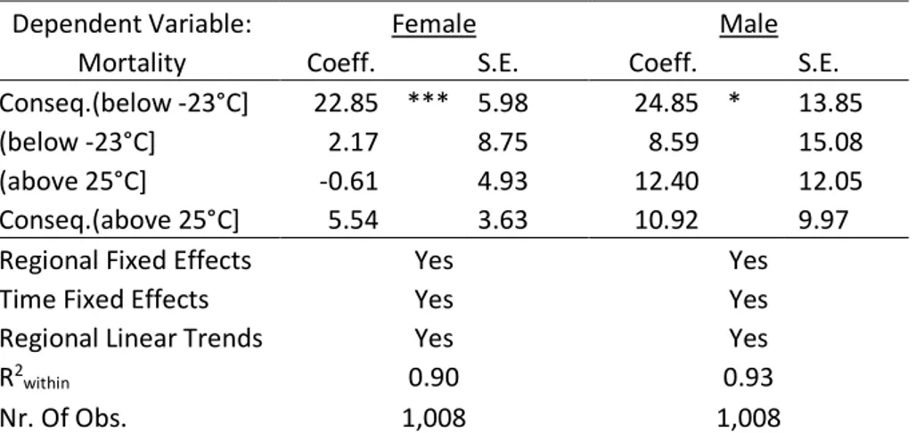
One of the central questions regarding climate change is whether individuals in warm and cold places can adapt to changing temperatures. Previous studies suggest that there might be heterogeneous effects of warm/cold days in warm/cold regions (Deschênes and Moretti, 2009; Heutel et al., 2017; Otrachshenko et al., 2017). To analyze this, we split our sample in half based on (i) the frequency of days above 25°C and (ii) the frequency of days below -23°C. In this section we present the results on the impact of weather in regions with high frequency of hot (warm regions) and cold (cold regions) temperatures. Note that our model includes the regional fixed effects, and as a result, those effects may subsume permanent adaptation that a warm or cold region has undertaken for its climate. Yet, the number of consecutive days may change even in those regions that have faced those days frequently.11_{For the sake of space, the results are} presented only for the single and consecutive extremely hot/cold temperature bins in Tables 7 and 8.

Tables 7 and 8 show the impacts of single and consecutive days with temperature below -23°C and above 25°C in warm and cold regions on the all-cause mortality in females and males, respectively. We find that in warm regions, neither single nor consecutive hot days affect the total mortality in females and in males (Table 7). On the other hand, in cold regions, both genders suffer from consecutive hot days (Table 8). Overall, these results suggest that in warm regions both genders have adapted to hot temperatures.

We also analyze the consequences of extremely cold temperatures. In warm regions, consecutive cold days increase the mortality of both genders while in cold regions, these days increase the mortality of females. This suggests that males adapt to cold days if those days occur frequently. For instance, such adaptation might happen as a result of risk-averse behavior that involves wearing warm clothes, staying indoors, and limiting the time of outdoor work (Donaldson et al., 1998a, 1998b). These results underscore

(20)

20 the importance of taking into account the impact of consecutive days with extremely cold temperatures on mortality in warm regions. Interestingly, the cold temperature impact in warms regions might be harmful as much as the impact of hot temperatures in cold regions.

Table 7: The impacts of a single day and a consecutive day with a specific temperature on the total all-age mortality in warm regions

Dependent Variable: Female Male

Mortality Coeff. S.E. Coeff. S.E. Conseq.(below -23°C] 22.85 *** 5.98 24.85 * 13.85

(below -23°C] 2.17 8.75 8.59 15.08

(above 25°C] -0.61 4.93 12.40 12.05

Conseq.(above 25°C] 5.54 3.63 10.92 9.97

Regional Fixed Effects Yes Yes

Time Fixed Effects Yes Yes

Regional Linear Trends Yes Yes

R2

within 0.90 0.93

Nr. Of Obs. 1,008 1,008

Notes: This model includes all temperature and precipitation bins as in Eq. (1). Robust standard errors are clustered at a regional level. The regional population weights are applied. The temperature bin (19°C, 22°C] and the precipitation bin [0 mm, 10 mm) are used as a default. ***, **, * stand for 1%, 5%, and 10% significance levels, respectively.

Table 8: The impacts of a single day and a consecutive day with a specific temperature on the total all-age mortality in cold regions

Mortality Coeff. S.E. Coeff. S.E. Conseq.(below -23°C] 11.47 *** 3.38 9.62 6.66

(below -23°C] -2.19 5.25 -5.50 9.77

(above 25°C] 0.90 9.24 -13.19 23.94

Conseq.(above 25°C] 19.46 *** 3.60 29.54 *** 7.49

R2

within 0.93 0.93

Nr. Of Obs. 1,014 1,014

Notes: This model includes all temperature and precipitation bins as in Eq. (1). Robust standard errors are clustered at a regional level. The regional population weights are applied. The temperature bin (19°C, 22°C] and the precipitation bin [0 mm, 10 mm) are used as a default. ***, **, * stand for 1%, 5%, and 10% significance levels, respectively.

(21)

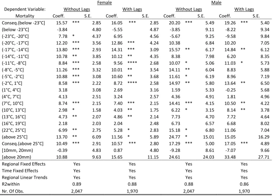
21 Using the region-by-year data on mortality typically helps to capture harvesting effects in the impact of temperature on mortality throughout the year (Deschênes and Greenstone, 2011).12_{To test that our model} adequately captures the end-of-year harvesting effect, i.e. the case when days with the November-December temperature of one year contribute to the mortality of the next year, we include one-year lags of all temperature and precipitation in addition to contemporary ones. If there is no statistical difference between contemporary estimates in the models with and without lags, then the models account for the end-of-year harvesting effect accurately. As shown in Table A.1 in the Appendix, this is confirmed for models with one-day and with consecutive day bins for both genders.

Early 1990s is a period of economic transition in Russia which is characterized by social and economic changes that also had an impact on mortality. Our model controls for regional and year fixed effects as well as linear regional trends that help to sufficiently capture potential changes related to transition period. We also divide our sample into transition (1989-1999) and post-transition (2000-2014) periods. The results suggest that estimates based on the full sample, transition, and post-transition periods are not statistically different from each other.13

We also estimate the model with an alternative specification of consecutive day bins. We redefine hot and cold consecutive day bins as follows. The hot consecutive day bin contains the number of sequences of three consecutive days with a daily mean temperature above 25°C and zero otherwise. In this case, four consecutive days are counted as two events within the hot consecutive day bin. Similarly, the cold consecutive bin contains the number of sequences of three consecutive days with a mean daily temperature below -23°C and zero otherwise. Yet, it is worth mentioning that with such specification, a four day event and two three-day events would be counted as the same thing even though the dynamics might be quite

12_{When daily data on mortality are available, to mitigate harvesting effects, the distributed lag model is often used.}

This model includes the temperature bins of previous days (Cohen and Dechezleprêtre, 2017; Deschênes and Moretti, 2009).

(22)

22 different.14_{The results for females and males are presented in Table A.2. As shown in this table, redefining} the consecutive temperature bins does not change the main findings.

Note that more than half of the total mortality in Russia is due to cardiovascular diseases.15_{The results} on the impacts of single and consecutive days, both cold and hot, on the cardiovascular-cause mortality are similar to the impact on the total all-age mortality. Those results are presented in Table A.3 in the Appendix.

5. Conclusion

This paper underscores the importance of accounting for the impacts of both single and consecutive days with extreme temperatures on mortality. We provide evidence that both consecutive hot and consecutive cold days increase mortality in all age and gender groups of the population, and males are affected more severely. Moreover, when the impacts of single and consecutive days are disentangled, we find that single hot days increase mortality, while single cold days do not affect mortality. These results suggest interesting policy implications, since with global warming, excess mortality due to the increasing number of extreme hot single and consecutive days may be partially mitigated by declining mortality due to the decreasing number of consecutive cold days. Given the vast climatic differences and uniform data collection in Russia, the findings can be useful to other regions that have started to face or will face extreme hot and cold temperatures in the future.

The results outline several avenues for future research. First, we provide evidence that consecutive days result in substantial losses of lives. This result has a number of social and economic implications also for other aspects of human life and behavior, e.g. for labor productivity (Zivin and Neidell, 2014) or crime (Ranson, 2014). Analyzing how consecutive days affect human behavior yet remains an open question that raises important implications for policies.

14_{We thank an anonymous referee for this comment.}

15_{In our sample, 54.2% of all deaths in Russia in the period 1989-2014 are due to cardiovascular diseases. For females,}

(23)

23 Second, given that the frequency and severity of both hot and cold extreme weather events will increase in the future (IPCC, 2014), it would be interesting to analyze whether the adaptation occurs with an increase in the length of consecutive extreme days. Third, our estimates present a lower bound of the impact of hot temperature, since most regions in Russia have frequently experienced average daily temperatures above 25°C, but have not yet frequently experienced average daily temperatures above 28°C. The frequency of extremely hot days is likely to increase with climate change, so it would be interesting to analyze the impact of days with higher temperature.

References

Ásgeirsdóttir, T.L., Corman, H., Noonan, K., Reichman, N.E., 2016. Lifecycle effects of a recession on health behaviors: Boom, bust, and recovery in Iceland. Economics and Human Biology 20, 90–107.

Barreca, A., Clay, K., Deschênes, O., Greenstone, M., Shapiro, J.S., 2016. Adapting to climate change: The remarkable decline in the US temperature-mortality relationship over the 20th century. Journal of Political Economy 124, 105–159.

Barreca, A., Clay, K., Deschênes, O., Greenstone, M., Shapiro, J.S., 2015. Convergence in adaptation to climate change: Evidence from high temperatures and mortality, 1900--2004. The American Economic Review 105, 247–251.

Barreca, A.I., 2012. Climate change, humidity, and mortality in the United States. Journal of Environmental Economics and Management 63, 19–34.

Basu, R., 2009. High ambient temperature and mortality: a review of epidemiologic studies from 2001 to 2008. Environmental health 8, 40.

Basu, R., Samet, J.M., 2002. Relation between elevated ambient temperature and mortality: A review of the epidemiologic evidence. Epidemiologic Reviews 24, 190–202.

Burgess, R., Deschenes, O., Donaldson, D., Greenstone, M., 2017. Weather, climate change and death in India. mimeo.

(24)

24 Burroughs, H.E., Hansen, S.J., 2011. Managing indoor air quality, 5th ed. Fairmont Press, Lilburn, GA. Cohen, F., Dechezleprêtre, A., 2017. Mortality, temperature, and public health provision: Evidence from

Mexico. mimeo.

Crost, B., Friedson, A., 2017. Recessions and health revisited: New findings for working age adults. Economics and Human Biology 27, 241–247.

Dell, M., Jones, B.F., Olken, B.A., 2014. What do we learn from the weather ? The new climate–economy literature. Journal of Economic Literature 52, 740–798.

Deschenes, O., 2014. Temperature, human health, and adaptation: A review of the empirical literature. Energy Economics 46, 606–619.

Deschênes, O., Greenstone, M., 2011. Climate change, mortality, and adaptation: Evidence from annual fluctuations in weather in the US. American Economic Journal: Applied Economics 3, 152–185. Deschênes, O., Moretti, E., 2009. Extreme weather events, mortality, and migration. The Review of

Economics and Statistics 91, 659–681.

Donaldson, G.C., Ermakov, S.P., Komarov, Y.M., McDonald, C.P., Keatinge, W.R., 1998a. Cold related mortalities and protection against cold in Yakutsk, eastern Siberia: observation and interview study. BMJ (Clinical research ed.) 317, 978–982.

Donaldson, G.C., Tchernjavskii, V.E., Ermakov, S.P., Bucher, K., Keatinge, W.R., 1998b. Winter mortality and cold stress in Yekaterinburg, Russia: interview survey. BMJ (Clinical research ed.) 316, 514–518. Falconi, A., Gemmill, A., Karasek, D., Goodman, J., Anderson, B., Lee, M., Bellows, B., Catalano, R., 2016.

Stroke-attributable death among older persons during the great recession. Economics and Human Biology 21, 56–63.

Gasparrini, A., Armstrong, B., 2011. The impact of heat waves on mortality. Epidemiology 22, 68–73. Gosling, S.N., Lowe, J.A., Mcgregor, G.R., Pelling, M., Malamud, B.D., 2009. Associations between elevated

atmospheric temperature and human mortality : a critical review of the literature. Climatic Change 92, 299–341.

(25)

25 Hajat, S., Armstrong, B., Baccini, M., Biggeri, A., Bisanti, L., Russo, A., Paldy, A., Menne, B., Kosatsky, T., 2006a. Impact of high temperatures on mortality: is there an added heat wave effect? Epidemiology 17, 632– 638.

Hajat, S., Armstrong, B., Baccini, M., Biggeri, A., Bisanti, L., Russo, A., Paldy, A., Menne, B., Kosatsky, T., 2006b. Impact of high temperatures on mortality: is there an added heat wave effect? Epidemiology 17, 632– 638.

Hanigan, I., Hall, G., Dear, K.B.G., 2006. A comparison of methods for calculating population exposure estimates of daily weather for health research. International journal of health geographics 5, 38. Heutel, G., Miller, N., Molitor, D., 2017. Adaptation and the Mortality Effects of Temperature Across U.S.

Climate Regions, NBER Working Paper 23271.

Huynen, M.M.T.E., Martens, P., Schram, D., Weijenberg, M.P., Kunst, A.E., 2001. The impact of heat waves and cold spells on mortality rates in the Dutch population. Environmental Health Perspectives 109, 463– 470.

Intergovernmental Panel on Climate Change (IPCC), 2014. Future climate changes, risk and impacts, in: The Core Writing Team, Pachauri, R.K., Meyer, L. (Eds.), Climate Change 2014: Synthesis Report. Contribution of Working Groups I, II and III to the Fifth Assessment Report of the Intergovernmental Panel on Climate Change. IPCC, Geneva, Switzerland, 56–74.

Martens, W.J.M., 1998. Climate change, thermal stress and mortality changes. Social Science and Medicine 46, 331–344.

McGeehin, M., Mirabelli, M., 2001. The potential impacts of climate variability and change on temperature-related morbidity and mortality in the United States. Environmental health perspectives 109 Suppl, 185–189.

Molina, O., Saldarriaga, V., 2017. The perils of climate change: In utero exposure to temperature variability and birth outcomes in the Andean region. Economics and Human Biology 24, 111–124.

(26)

26 Economics 132, 290–306.

Pattenden, S., Nikiforov, B., Armstrong, B.G., 2003. Mortality and temperature in Sofia and London. J Epidemiol Community Health 57, 628–633.

Portnykh, M., 2017. The effect of weather on mortality in Russia: What if people adapt? mimeo.

Poumadère, M., Mays, C., Le Mer, S., Blong, R., 2005. The 2003 heat wave in France: Dangerous climate change here and now. Risk Analysis 25, 1483–1494.

Ranson, M., 2014. Crime, weather, and climate change. Journal of Environmental Economics and Management 67, 274–302.

Revich, B., Shaposhnikov, D., 2012. Climate change, heat waves, and cold spells as risk factors for increased mortality in some regions of Russia. Studies on Russian Economic Development 23, 195–207.

The World Bank, 2016. Average monthly Temperature and Rainfall for Russia from 1990-2012. Climate

Change Knowledge Portal. The World Bank Group. URL

http://sdwebx.worldbank.org/climateportal/index.cfm?page=country_historical_climate&ThisCCode= RUS (accessed 7.15.16).

Zivin, J.G., Neidell, M.J., 2014. Temperature and the allocation of time: Implications for climate change. Journal of Labor Economics 32, 1–26.

(27)

27

Appendix

Table A.1: Models with and without lags of temperature and precipitation bins

Female Male

Dependent Variable: Without Lags With Lags Without Lags With Lags

Conseq.(below -23°C] 15.57 *** 2.85 16.05 *** 2.85 20.20 *** 5.49 19.26 *** 5.40 (below -23°C] -3.84 4.80 -5.55 4.87 -3.85 9.11 -8.22 9.34 (-23°C, -20°C] 7.78 * 4.37 6.95 4.56 -5.67 9.25 -9.58 9.84 (-20°C, -17°C] 12.20 *** 3.56 12.86 *** 4.24 10.38 6.84 10.20 7.05 (-17°C, -14°C] 13.80 *** 2.93 14.31 *** 3.09 15.57 ** 6.17 14.84 ** 6.12 (-14°C, -11°C] 10.78 ** 3.85 10.12 ** 4.35 8.38 7.98 6.20 8.35 (-11°C, -8°C] 8.84 *** 2.58 9.56 **** 2.68 10.07 * 5.06 11.03 * 5.73 (-8°C, -5°C] 11.26 *** 3.32 10.01 ** 3.54 14.11 ** 6.04 8.83 5.88 (-5°C, -2°C] 10.88 *** 3.08 10.60 ** 3.68 11.61 * 6.19 8.96 7.19 (-2°C, 1°C] 8.58 *** 2.22 8.72 **** 2.58 14.97 ** 5.80 13.64 ** 6.50 (1°C, 4°C] 3.18 3.08 2.69 3.16 1.59 5.33 -0.25 5.68 (4°C, 7°C] 4.13 2.51 3.24 2.57 4.36 4.91 1.81 4.96 (7°C, 10°C] 8.74 *** 2.15 7.40 *** 2.15 14.41 *** 4.15 10.50 ** 4.22 (10°C, 13°C] 2.98 * 1.58 4.03 ** 1.75 6.22 * 3.15 8.14 ** 3.78 (13°C, 16°C] 4.73 ** 2.07 4.86 ** 2.14 7.73 4.70 7.72 4.64 (16°C, 19°C] 2.18 2.03 2.04 2.48 6.73 6.57 6.68 8.02 (22°C, 25°C] 6.99 ** 2.75 5.28 * 2.83 15.18 * 6.80 11.06 7.04 (above 25°C] 13.70 ** 6.09 11.56 * 5.89 24.77 * 15.01 15.05 16.29 Conseq.(above 25°C] 10.49 *** 2.91 10.57 *** 2.80 17.29 *** 5.00 17.05 *** 4.89 [10mm, 20mm) -0.39 4.83 0.87 4.80 -9.28 8.61 -7.07 9.66 [above 20mm) 10.88 9.63 15.65 11.15 24.61 24.03 33.48 27.71

R2within 0.89 0.88 0.88 0.86

Nr. Of Obs. 2,047 1,970 2,047 1,970

Notes: Models present the results of the combined specification that includes both single and consecutive day effects for females and males, respectively.

Models with lags include one-year lags of all temperature and precipitation in addition to contemporary ones.Robust standard errors are clustered at a regional level. The regional population weights are applied. The temperature bin (19°C, 22°C] and the precipitation bin [0 mm, 10 mm) are used as a default. ***, **, * stand for 1%, 5%, and 10% significance levels, respectively.

(28)

28 Table A.2: Model with an alternative specification of consecutive days

Mortality Coeff. S.E. Coeff. S.E. Conseq.(below -23°C] 15.02 *** 3.82 16.30 ** 6.85 (below -23°C] 0.64 4.90 2.78 9.02 (-23°C, -20°C] 7.86 * 4.63 -7.46 9.57 (-20°C, -17°C] 10.92 *** 3.69 7.45 7.01 (-17°C, -14°C] 12.45 *** 3.07 12.51 ** 6.26 (-14°C, -11°C] 9.17 ** 3.83 5.20 8.04 (-11°C, -8°C] 7.86 *** 2.65 7.56 5.21 (-8°C, -5°C] 10.43 *** 3.36 12.04 * 6.04 (-5°C, -2°C] 9.74 *** 3.12 9.02 6.26 (-2°C, 1°C] 7.47 *** 2.27 12.40 ** 5.82 (1°C, 4°C] 2.34 3.07 -0.61 5.35 (4°C, 7°C] 3.60 2.54 2.88 4.95 (7°C, 10°C] 7.91 *** 2.20 12.56 *** 4.17 (10°C, 13°C] 2.45 * 1.63 4.69 3.34 (13°C, 16°C] 4.17 2.09 6.16 4.73 (16°C, 19°C] 1.76 ** 2.09 5.24 6.60 (22°C, 25°C] 6.88 ** 2.90 13.78 * 7.16 (above 25°C] 14.33 ** 6.32 28.92 * 14.70 Conseq.(above 25°C] 11.82 *** 4.10 16.13 ** 6.79 [10mm, 20mm) -0.17 4.92 -9.25 8.68 [above 20mm) 10.65 9.74 23.87 24.08

R2

within 0.89 0.87

Nr. Of Obs. 2,047 2,047

Notes: Models present the results of the combined specification that includes both single and consecutive day effects for females and males, respectively. Robust standard errors are clustered at a regional level. The regional population weights are applied. The temperature bin (19°C, 22°C] and the precipitation bin [0 mm, 10 mm) are used as a default. ***, **, * stand for 1%, 5%, and 10% significance levels, respectively.

(29)

29

Table A.3: The impacts of single and consecutive day with a specific temperature on the cardiovascular all-age mortality

Model: (1a) (1b) (2a) (2b)

Dependent Variable: Female Male Female Male

Conseq.(below -23°C] - - 12.14 *** 3.31 12.18 *** 3.40 (below -23°C] 14.32 *** 3.37 19.75 *** 4.29 -2.52 6.63 6.93 6.01 (-23°C, -20°C] -0.60 6.09 -1.02 5.77 -0.06 5.88 -1.65 5.94 (-20°C, -17°C] 16.96 *** 4.26 14.05 ** 4.46 15.13 *** 4.30 11.13 ** 4.36 (-17°C, -14°C] 11.39 *** 3.70 14.92 *** 3.62 8.85 ** 3.75 11.33 *** 3.33 (-14°C, -11°C] 14.85 *** 3.82 14.95 3.76 12.68 *** 3.73 11.75 *** 3.76 (-11°C, -8°C] 9.39 ** 3.41 10.46 ** 2.65 7.42 ** 3.42 7.67 *** 2.77 (-8°C, -5°C] 12.76 *** 3.72 14.44 *** 3.71 10.82 ** 3.88 11.77 *** 3.83 (-5°C, -2°C] 13.30 ** 3.14 11.92 ** 3.56 11.50 *** 2.93 9.29 ** 3.34 (-2°C, 1°C] 9.21 *** 2.74 10.73 *** 2.85 7.79 ** 2.85 8.45 ** 3.16 (1°C, 4°C] 5.84 * 3.27 6.81 2.51 4.35 3.42 4.61 2.76 (4°C, 7°C] 9.69 *** 2.87 8.17 2.81 8.18 *** 2.78 6.12 ** 2.79 (7°C, 10°C] 9.26 *** 3.03 12.84 *** 2.41 8.28 ** 2.91 11.20 *** 2.45 (10°C, 13°C] 3.15 2.18 4.50 ** 1.90 2.44 2.21 3.27 * 1.93 (13°C, 16°C] 3.73 ** 1.78 4.15 * 2.23 3.27 * 1.85 3.28 2.33 (16°C, 19°C] 5.33 ** 2.10 4.62 3.06 4.53 2.13 3.52 3.22 (22°C, 25°C] 5.44 3.41 4.72 ** 3.65 4.86 ** 3.75 4.03 3.95 (above 25°C] 11.84 *** 3.15 9.06 *** 3.17 22.63 ** 11.13 9.82 8.16 Conseq.(above 25°C] - - 8.97 *** 3.03 7.17 *** 3.19 [10mm, 20mm) 3.25 4.56 -0.77 4.09 3.37 4.45 -0.68 4.12 [above 20mm) 9.13 11.34 10.01 14.20 9.14 11.21 10.16 14.02

R2

within 0.77 0.86 0.77 0.86

Nr. Of Obs. 2,043 2,043 2,043 2,043

Notes: Models 1a and 1b present the results with single day effects for females and males, respectively. Models 2a and 2b present the results of the combined

specification that includes both single and consecutive day effects for females and males, respectively. Robust standard errors are clustered at a regional level. The regional population weights are applied. The temperature bin (19°C, 22°C] and the precipitation bin [0 mm, 10 mm) are used as a default. ***, **, * stand for 1%, 5%, and 10% significance levels, respectively.