Stock price and cost of debt reaction to changes in cash flow from operations

M

ASTER IN

F

INANCE

M

ASTERS

’

F

INAL

W

ORK

D

ISSERTATION

S

TOCK

P

RICE AND

C

OST OF

D

EBT REACTION TO

C

HANGES IN

C

ASH

F

LOW

F

ROM

O

PERATIONS

SHUJA'A

AHMAD

ABDELFATTAH

HIASAT

M

ASTER IN

FINANCE

M

ASTERS

’

F

INAL

W

ORK

D

ISSERTATION

S

TOCK

P

RICE AND

C

OST OF

D

EBT REACTION TO

CHANGES IN

C

ASH

F

LOW

F

ROM

O

PERATIONS

SHUJA'A

AHMAD

ABDELFATTAH

HIASAT

S

UPERVISOR

:

P

ROFESSOR

D

OUTOR

T

IAGO

C

RUZ

G

ONÇALVES

i

Abstract

We investigate how the Cash Flow from Operations affects both the Stock Price

Return and the Cost of Debt and compare the relative effect of Cash Flow versus Net

Income on both costs of financing. This paper also compares the liquidity between

STOXX Europe 600 and Amman stock exchange 100 (ASE100) indexes using four

measures, Cash Flow from Operations, Market Adjusted Return, Cumulative Abnormal

Return, and the Cost of Debt and its relative impact on Cash flow association with cost

of capital. The quarterly data used for this research comes from publicly listed firms from

Jordan and European countries, from 2009 through 2018. This study contributes to

literature since it provides evidence on the relative association of Earnings and cash flows

with cost of debt and stock returns. We are also the first to consider any market liquidity

effect on this association.

The results show a positive effect of Cash Flow from Operations on Stock Price

Returns. It also shows a negative association and a more significant influence from Cash

Flow from Operations than Net Income on the Cost of Debt, by reducing it. Furthermore,

the paper also shows Cash Flow from Operations tend to influence the Cumulative

Abnormal Return and the Cost of Debt in a better way in Jordan (a less liquid market)

than in the more developed European market.

Keywords: Cash Flow from Operation; Net Income; Stock Price Return; Cost of Debt;

Liquidity.

ii

List of Abbreviations

ABNRET – Cumulative Abnormal Return ADJ_COST – Adjusted Cost of Debt CFO – Cash Flow from Operations MKTADJRET – Market Adjusted Return N.I – Net Income

iii

Acknowledgments

This paper marks an important milestone that I achieved, namely the conclusion of my Masters’ Degree. This was only possible with the tremendous support I had from a group of people.

First, I would like to thank Professor Tiago Gonçalves, for pointing me in the right direction, for the constant confidence and encouragement always offered along the way, the availability shown and share of knowledge. Besides his focus on specific details which improved my knowledge, my way of writing, and my way of research.

Also, I am grateful to my friends, the Jordanian friends and my friends at ISEG School, they always encouraged me and made me feel that I can do anything amazing in this life. I would like to thank my family, for always caring and showing interest during my study and my research.

iv

Contents

1. INTRODUCTION

... 1

2. LITERATURE REVIEW

... 2

3. RESEARCH QUESTION AND HYPOTHESES

... 8

3.1. Hypotheses Development ... 8

4. RESEARCH METHODOLOGY

... 9

5- RESULTS

... 17

5.3.1. Market Adjusted Return (MKTADJRET) ... 20

5.3.2. Cumulative Abnormal Return (ABNRET) ... 21

5.3.3. Adjusted Cost of Debt (ADJ_COST) ... 22

5.4. Comparing the liquidity between STOXX Europe 600 and ASE100 indexes ... 24

6- CONCLUSION

... 31

7- REFERENCES

... 33

v

List of Tables

T

I-

N

S

... 17

T

III-T

J

CFO/SALES

E

CFO/SALES

... 18

T

IV-T

J

CFO/SALES

E

CFO/SALES

... 19

T

V-R

1(MKTADJRET)

... 20

T

VI-R

1

(ABNRET)

... 21

T

VII-R

A

2

... 22

T

VIII-

MKT

MKT*CFO/SALES

MKTADJRET

... 24

T

IX-

MKT

MKT*CFO/SALES

ABNRET

.. 25

T

X-

MKT

MKT*CFO/SALES

C

D

... 26

T

XI-

D

MKTADJRET,

ABNRET,

ADJ_COST

... 28

T

XII-T

MKTADJRET

J

E

... 28

T

XIII-

T

ABNRET

J

E

... 29

T

XIV-

T

ADJ_COST

J

E

... 30

T

XV-

N

S

... 37

T

XVII-D

... 39

T

XVIII-C

E

1

... 40

1

1. Introduction

Multiple factors affect Stock Prices and Cost of Debt. For example, economic situations, country status and regulations, the size of the company, and financial reporting. Many previous studies discussed analyzing the company’s financial statements and how they can affect the Stock Prices and Cost of Debt in the capital market considering liquidity, solvency, and profitability analysis.

Investors look at the financial statements and the data that are published to the public by focusing mainly on the Net Income, paying less attention to the Cash Flow from Operations that explains how a company can have positive cash balance from its day-to-day events, so it is able to finance itself from the main source of business revenue and to have better access to the capital market. This may lead to Earnings fixation rather than a rational maximization of Cash flow (Gonçalves, Gaio & Lelis, 2020).

Extent literature discusses different arguments about the preferences of using Net Income and Cash Flow from the Operations as a measure of the firm market performance. Liu, Nissim, & Thomas (2007) prefer to use net income and they consider it the king for valuing the firm, while Martani, Mulyono & Khairurizka (2009) say that both Net Income and Cash Flow from Operations affect positively on the stock price return, but the higher effect comes from net income. Largay III & Stickney (1980), and Catanach (2000) notice that, on the long run, the effect of the Cash Flow from the Operations will beat the effect of Net Income. The lower the amount of Cash Flow from Operations, the lower will be the stock price return and the higher the Cost of Debt that will be charged to the firm.

This study aims to analyze how the Cash Flow from Operations affects the stock price return, comparing this effect with that of Net Income on the stock returns as well as on the Cost of Debt. We also analyze market liquidity impact on those associations, namely by comparing between STOXX Europe 600 versus Amman stock exchange 100. The quarterly data used in our sample is collected from both the STOXX Europe 600 and Amman stock exchange 100 from the period 2009-2018.

We find that Cash Flow from Operations affects positively the stock price return and this effect is higher than that of the Net Income (similarly to (Graham & Knight, 2000)), yet the higher effect of Cash Flow from Operations is not statistically significant. On the other hand, Cash Flow from Operations affects negatively on the Cost of Debt- by reducing it, and this effect is more significant than from Net Income. In addition, we compare between STOXX Europe 600 and Amman stock exchange 100 indexes. we find that STOXX Europe 600 is more liquid than Amman stock exchange 100 indexes, STOXX Europe 600 has higher returns and lower cost of Debt, and the Cash Flow from Operations generated by STOXX Europe 600 is more able to

2

increase the Market adjusted returns, but the Cash Flow from Operations generated by Amman stock exchange 100 is more able to increase the Cumulative abnormal return and reduces the cost of Debt by more than the amount generated from STOXX Europe 600.

Our paper contributes to the literature by specifically addressing the differential effect of Cash flow and Net income on Cost of Debt and Stock returns. We show that the impact of Cash flow is higher for both debt holders and stock holders, but it is only robustly significant in the former. We also contribute to show the moderating effect of market liquidity and stock market development on this association. We show that the relative importance of Cash flow on cost of debt is more significant in less liquid markets. These results matter both for investors (stock and debtholders when allocating portfolio budgets) but also for regulators, that should consider the differential impacts of disclosed information on different stakeholders.

The remainder of the paper is divided into different sections: section 2 presents the literature review, section 3 presents the research question and hypotheses, section 4 presents the research methodology, section 5 presents the results, and section 6 presents the conclusion.

2. Literature Review

Money providers look at the financial statements’ items and the data that are published to the public, which are based on Accrual Accounting. These items make an effect on borrowing and investment decisions. Cash Flow from Operations, that explains how a company can have positive cash balance from its day-to-day events so it is able to finance itself from the main source of business revenue and to have better access to the capital market. This study focuses mainly on four financial items: Net Income, Cash Flow from Operations, Stock Price Return, and Cost of Debt, assome past studies provide evidence about the interaction of Stock Price Return and Cost of Debt with the Cash Flow from Operations, as well as the Stock Price and Cost of Debt relationships with Net Income alone, but results are mixed and research usually considers only individual impact on one the investment type decisions.

Income Statement is one of the financial statements that is used to give a clear understanding of a company's performance over a given period. The presentation of the Income Statement is done by deducting the total expenses from the total revenue to reach the earnings amount; so Net Income (N.I) is the sum of items recognized as revenues minus the sum of items recognized as expenses, except incomes and expenses transferred to the statement of comprehensive income

(Bogle, 2018; Barker, 2010). The International Accounting Standard Board (IASB) identifies N.I

as an increase in economic benefits during the accounting period in the form of inflows, enhancements of assets or decreases of liabilities that result in increases in equity, other than those relating to contributions from equity participants. This is the most used item for valuing the

3

performance of the firm, and one of the earnings components people care about since it has an important influence on securities returns (Cheng, Cheung, & Gopalakrishnan , 2013).

Hicksian’s Income Theory indicates that the purpose of showing the income amount is to present the amount firms can consume without being in a deficit. This theory talked about both the personal income that shows the ability of the person to spend the amount she has within a week, and the amount of profit that is in the hand of the company’s shareholders after considering the amount of expenses to deduct total revenues (Jameson, 2005).

N.I comes from all the changes in the economic value of the firm that result from repeated activities and circumstances. It can be used as an important measure to predict the future profit and the value of the firm since most of the revenues and expenses transactions repeat themselves in the same way inside the business (Kanagaretnam, Mathieu, & Shehata, 2009) .The change in the amount of earnings reported for a company shows a huge market interaction to that change, so the improvement in the amount of earnings announced increases the investors demand for company’s shares and drive up the stock price for the firm (Francis, Schipper, & Vincent, 2002).

International Accounting Standard No. 7 (IAS No. 7) defines the operating activities as events that include day- to- day activities and create revenues, such as selling inventory and providing services. Cash inflows result from cash sales and collection of accounts receivable. Examples include cash received from the provision of services and royalties, commissions, and other revenues. To generate revenue, companies undertake activities such as manufacturing inventory, purchasing inventory from suppliers, and paying employees. Cash outflows result from cash payments for inventory, salaries, taxes, accounts payable, and other operating related expenses. Casey and Bartczak (1985) define Cash Flow from Operations (CFO) as the change in operating working capital added or deducted to any change in the non-cash working capital operation plus Net Income, except for short term debt and the current portion of long term debt.Many textbooks use this definition (Rai, 2003). Austin and Bradbury (1995) add a classification for CFO. They define it as the net cash amount that results from the cash collected from customers, cash paid to suppliers, cash paid for taxes, cash paid for interest, and cash changes in other operating activities.

Hanini and Abdullatif (2013) provide a study in Jordan that discussedwhether the Jordanian auditors are giving a significant importance to understand the items published in the statement of cash flow for measuring the going concern of the firm. They state that the auditors must be well knowledgeable about the statement of cash flow as an important role for the professional responsibilities of audit firms; otherwise, this will lead to fraud by the firm and losing clients’ trust.

Utomo and Pamungkas (2018) specify how Cash Flow from Operating Activities (CFO), Cash Flow from Investing Activities (CFI), and Cash Flow from Financing Activities (CFF) affect

4

the stock returns. They include that the analysts should carefully consider how firms operate CFO regarding the economic activities. This leads to CFO is an important factor, that can make huge changes on the economic decisions made by managers, investors, creditors, and any other users of the financial statements, since it is an evidence of real cash on hand collected from the main source of the business during the period. Thus, it is one of the best items to use in measuring performance and liquidity of the firm (Jones & Ratnatunga, 1997).

The amount of earnings reported is a component that plays a significant role in the valuation of the economic events of the firm (Kanagaretnam, Mathieu, & Shehata, 2009). However, if we classify the cash balance of the firm into operating, investing, and financing balances, we will observe that the CFO amount and its components are major in understanding the economic activities of the firm, since they are evidence of the strong operational sources the firm owns, and they reflect the ability of the firm to make internal funding from its daily activities. Therefore, they significantly and positively affect the stock price return more than the amount provided by N.I ( Livnat & Zarowin, 1990).

Laitine (1994) made a comparison between traditional cash flow (N.I added to the depreciation expenses) and the CFO reported in the statement of cash flow by dividing each of the two items on total debt. This comparison was between two groups of firms, bankrupted firms and non-bankrupted firms. He found that the traditional cash flow is a more stable and reliable predictor of failure than the CFO reported. The firm that has signs of bankruptcy will have decreasing N.I overtime. However, CFO is more sensitive to the management of accounts receivables, inventory, and accounts payables. Weak management of these operational assets and liabilities could include a warning for the firm to enter in solvency problems, even if the negative CFO is just for a temporary or special period. This analysis agrees with Largay III & Stickney (1980) who conducted a study on W.T Grant Company to understand the reasons why the company had been in bankruptcy. They found that W.T Grant Company was improving in stock price movements and earnings, but at the same time, it was achieving a negative CFO balance during a period, which made the company facing bankruptcy on the long run. In addition, Casey and Bartczak (1985) make a comparison between firms that entered bankruptcy and firms that did not enter bankruptcy. They conclude that the accrual-based ratios are better predictors for failure than the CFO ratios, but they suggest that the CFO ratios may have alternative uses, analyzing bank loan default, unpaid dividends, and any other uses related to the financial situation of the firm.

The good quality of Net Income, which the company generates, will result in a positive CFO. If we return to a hypothetical Company that was achieving a higher amount of N.I, but a negative CFO, we will find that the company was financing itself using debt. This transaction made the

5

company have negative cash flow in the long run, which was unable to be paid (Gaugha, Fuentes, & Bonanomi, 1995).

Graham & Knight (2000) argued about the amount of reported N.I and the CFO. Although the N.I is a component of the CFO, and both are highly correlated with each other, they say that the CFO balance is more able to change the movements of both the stock price and the stock price return, because Net Income is based on accrual accounting. Therefore, it can be more manageable by Management, while these accruals are adjusted to arrive at the CFO balance. As so, the CFO is less changeable, and it can be used as a real cash measure. However, Liu, Nissim, and Thomas (2007) prefer N.I over CFO. They say that earnings per share (EPS) forecasts represent better summary for valuation purposes in comparison to CFO, and N.I mentioned in the income statement is the king for valuing a company instead of using cash balance resulted from operations.

Recently, Jabbari, Sadeghi, & Askari (2013) talk in their study about stock price crash risk, in Tehran Stock Exchange, that the more the CFO balance, the lower will be the earnings opacity and thus the lower stock price crash risk. Earnings opacity is the lack of information reported in financial statements, which leads to distorting earnings recognized, and stock price crash risk is the probability of extreme negative stock price return.

Stock represents a share of ownership of a company. It is evidence of owning equity of this company. The Investor buys a stock hoping to obtain dividends income or that this stock will appreciate (Dmouj, 2006). The stock price is the highest price a person is willing to pay for purchasing a share or the lowest price the person is willing to sell that share. It shows the price at which the current stock is trading in the market. According to McCarroll & Khatri (2013), the fair value is the price that would be received to sell an asset or paid to transfer a liability in an orderly transaction between market participants at the measurement date. We can use this definition to describe the stock price because it is the price between the market participants that consists of the company issuing shares and the investor. It is used to calculate the total market value of equity outstanding by the firm (Foerster, Tsagarelis , & Wang, 2017).

Stock price return defines the percentage rate of return generated on holding the stock of the firm for a period of time. This is the return investor generates from the change in the market value of the stock by the appreciation in value, and from the additional amount of money received as dividends. It is the percentage increase in the stock price plus an income (Dmouj, 2006). Analysts use the holding period return (HPR) as a definition of the stock return achieved. HPR is the actual return that investors generate from holding the stock from the time of acquiring with a price (𝑃0),

6

Considering the effect of the N.I reported and keeping the other variables constant, the increase in the amount of N.I mentioned in the annual report will motivate the investor from his or her short memory. The current number is a measure of an improvement in the firm future performance, so she can benefit from the expected increase in the stock price by selling this stock later, and achieving a personal profit (Archibald, 2014). By analyzing each component of the CFO, which consists of N.I and working capital requirements items, we will realize that N.I, working capital requirements, and CFO balances, all significantly affect the securities return (Rayburn, 1986).

Forester, Tsagarelis,& Wang (2017) make a comparison between cash flow return on equity and assets ratios versus accrual profitability return on equity and assets ratios that use operating income and N.I. They find that cash flow ratios are better measures of profitability than the accrual returns ratio, because the CFO is an item that summarizes the clean economic events. They suggest more weight on the cash flow ratios for predicting the stock price returns than the accrual ratios, as they are more understandable by the investors and the analysts.

If theinvestor fails to identify the components of earnings as real cash earnings and accrual earnings, he will revert to the amount of N.I announced by the firm that is based on accrual recognition of revenues and expenses. Thus, he is overweighting accruals and underweighting cash flows, and the accruals could no longer predict the future stock prices, but if he can identify the CFO balance into N.I, Non-cash expenses, and changes in working capital requirements, he will recognize that each component has a significant effect on the stock price, since the stock price reflects the information of changes in these items (Gonçalves, Gaio, & Lélis, 2020).

CFO/N.I is a measure of how much operating cash isgenerated from each $1 of Net Income the company achieves. One prefers to increase this ratio because it is a measure of how much N.I is strong, but a lower amount of CFO and higher amount of N.I could be a sign of collecting accrued revenue or paying an accrued expense in the future. Moreover, changing the Accounting method used for inventory recognition (For example, from FIFO to LIFO or the opposite) may result in a negative N.I, but higher CFO balance. CFO balance is more able to affect positively the stock price.

By valuing the firm using the discounted earnings versus discounted free cash flow (FCF). Gaugha, Fuentes, & Bonanomi (1995) noticed that in case of an existing conflict between N.I and FCF, it is better to use the FCF for valuing the firm since it heavily counts on the CFO balance, which better affects the movements of the stock price.

The cost of Debt is the cost reflected by interest rate, thus, it is the interest charged to the company because of the money borrowed. It is the expense of borrowing from bank loans, bonds issued, and similar financial securities (Aomrah, 2011). Cost of Debt is the explicit cost that the

7

firm incurs from obtaining bank loans, issuing bonds, or if someone invests in the debt capital that the firm issues. If we divide the total capital to the part of the total debt and the total equity part, then the specialists use the Cost of Debt expression to analyze the opportunity cost related to the debt capital (Lehutová, Križanová, & Klieštik, 2013). On the opposite side, the cost of Debt explains the expected returns for the debt holders (Baule, 2019).

Edmonds, Edmonds, & Maher (2011) test the relationship between CFO and the Cost of Debt. From their research, they say that to improve in the firm bond rating, it needs to meet or beat the required N.I and CFO since both items positively affect the bond rating of the firm and the bond yield negatively. Therefore, this will reduce the cost of issuing bonds, and in this case, the firm can benefit from debt financing. They find that if the firm misses the N.I and CFO requirements, this will have a negative influence on their bond ratings more than the positive influence of meeting or beating N.I and CFO requirements. However, they could not find evidence whether the CFO measure is better than the N.I measure or the opposite. Nevertheless, they stated that the CFO is complementary to the N.I to make better movements in the firm bond rating.

A higher level of leverage will motivate the management to edit the way of recognizing N.I by changing the accounting policies used to prepare the financial report. This can happen by increasing sales, overproducing to increase the inventory amount and to lower the cost of sales, and reducing the selling and administrative expenses. All of the three ways will improve N.I. In this scenario, management can show the creditors and shareholders that they are in a good position based on N.I, and they can obtain debt funds at a lower cost (Zamri, AbdulRahman, & Isa, 2013).

Richardson (2006) mentions in the study of the relationship between Free Cash Flow (FCF) and over investments that if the firm faces a shortfall in the CFO balance, it would enter the capital market regarding equity or debt to finance its long-run operations; since it needs an outside provider of cash to achieve positive net present value (NPV). She did not mention in the study the effect of CFO balance on the cost of Debt, but she concluded that a positive CFO balance will have a positive FCF, which means that the cost of internal financing is lower than the cost of external financing, so the firm can use the positive FCF to keep it in the form of cash and marketable securities or to make an over investment.

Catanach (2000) suggested that managers, external auditors, and bankers should focus on CFO balance more than N.I and other accruals in measuring credit and interest rate risks. Negative CFO increases the probability of making the firm unable to pay the amount of interests required. This situation charges the firm a higher market interest rate because of the increase in the probability of being distressed, which influences negatively on the securities market value of Debt.

8

By talking about the ability of the corporation to finance itself without a significant loss in asset prices, Lancaster, Stevens, & Jennings (2002) try to replace the Current Ratio with the CFO. They find that CFO better explains the liquidity and Cash Conversion Cycle for the corporation. Additionally, CFO significantly influences these two ratios more than N.I and the Current ratio, because CFO explains the actual Cash that can be used to settle the liquidation needs and to measure the power of the liquidity.

3. Research Question and Hypotheses

As stated before, the CFO component uses a cash basis and represents the actual cash flow collected by the firm. Thus, it is less subject to deceive money providers, as compared to N.I that results from accrual accounting (Graham & Knight, 2000). If the internal financing is not sufficient to fund the long-run operations, the firm will find it necessary to use higher external financing costs as the only choice available. This leads the management to try using some accounting discretionary in a way that gives a nicer picture of N.I. This model provided from earnings reported makes it easier for the firm to enter the capital market since the investors and bankers are focusing on the amount presented in the income statement, where, for instance, less conservative management will increase Earnings Management (Aman , Iskandar, Pourjalali , & Teruya , 2006; Gonçalves & Coelho, 2019; Gonçalves, Gaio, & Santos, 2019; Gaio, Gonçalves, & Azevedo, 2020). Healy & Wahlen (1999) did not find a specific way managers can use to better communicate the firm’s performance to the investors. However, they mentioned that distorting N.I could make even a little difference in providing equity capital by investors.

So, our main research question to be investigated is: Which components of earnings are

more relevant to the stock and debt holders?

To answer this question, we will use the two components of earnings: CFO and N.I; andfour major relationships will be considered. Firstly, how the stock price return reacts to CFO. Secondly, comparing the effect between CFO and N.I on the Stock price return. Thirdly, how the cost of Debt reacts to the CFO. Fourthly, comparing the effect of CFO and N.I on the Cost of Debt. Fifthly, comparing the liquidity between STOXX Europe 600 index and Amman Stock Exchange 100 index (ASE100) and its impact on the aforementioned associations. The overall study will use quarterly data for the period from 2009 to 2018.

3.1. Hypotheses Development

3.1.1 CFO and Stock Price Return.

The CFO is an evidence of the strong operational sources the firm has. It reflects the ability of the firm to make internal funding from its daily activities. Besides that, it is one of the best measures that can be used to enter the capital market at a lower cost and it affects the stock price

9

return more than the amount provided from N.I ( Livnat & Zarowin, 1990). Thus, the first two hypotheses to be studied are the relationship between stock price and the CFO:

H1: - CFO associates positively with stock price returns.

H2: - CFO associates relatively higher than N.I with stock price returns.

3.1.2 CFO and Cost of Debt.

Calegari (2000) talks about the change in tax rules. This change affects both the accounting and financial policies that the firm follows. When the change harms the firm, it will try to improve the positive accrual income reported by changing the policies used to recognize expenses or revenues. The change in the accounting policies, discretionarily, creates more benefits since these changes present the ability to improve earnings. Therefore, it can avoid the requirements of higher interest rates by banks regarding an additional increase in the leverage ratios. Thus, the following two hypotheseswill be tested:

H3: - CFO associates positively with the Cost of Debt.

H4: - CFO associates relatively higher than N.I with the cost of Debt.

3.1.3 The liquidity of the market.

As we have collected data from the STOXX Europe 600 index, and ASE100 indexes, the following Hypothesis will be tested:

H5: - Market liquidity will moderate the association of CFO to Stock returns and Cost of Debt.

4. Research Methodology

To test the first two hypotheses, our first regression model is similar to what is used by Martani, Mulyono, & Khairurizka (2009) to measure the stock price return, since some of the financial ratios influence the stock price return:

RET=β₀+β₁NPM+ β₂ CFO

SALES+ β3 ROE+ β4 CR+β5DER+β6TATO+β7PBV + β8Log TA (1)

The first dependent variable consists of two measures: cumulative market-adjusted return and cumulative abnormal return. NPM is the net profit margin; 𝐶𝐹𝑂

𝑆𝑎𝑙𝑒𝑠 is the cash flow from operation

divided by total revenues; ROE is the return on equity; CR is the current ratio; DER is the debt to equity ratio; TATO is the total assets turnover; PBV is the price to book value per share, and Log TA is the measure of the size of the firm.

10

Our second regression model, to test H3 and H4, is similar to Alvarez-Botas & Gonzalez (2019), added by NPM and CFO/SALES as our two main independent variables for the study:

ADJ_COST_t=β₀+β₁NPM_T+β₂CFO/SALES_T+β₃LEV_T-1+β₄EBIT/INT_T-1

+ β₅MAT_T-1+β₆PROF_T-1+ β₇TANG_T-1+ β₈SIZE_T-1

+ β₉MTB_T-1+ β₁₀INF_T-1+ β₁₁R_LAW_T+ β₁₂LEG_IND_T

+ β₁₃R_LAW_T*LRG_IND T+ β14DEP_INFT + β₁₅DEP_INF_T*LRG_IND T+ β16B_CREDITT + β₁₇B_CONC_T+∈ (2)

Where ADJ_COST_t is the adjusted cost of debt; NPMT is the net profit margin; _SalesCFO is the

cash flow from operation divided by total revenues; LEV is the leverage ratio; EBIT/INTT-1 is the

earnings before interest and tax divided by total interest; MATT-1 is the long term debt divided by

total debt; PROFT-1 is the earnings before interest and tax divided by total assets; TANGT-1 is the

tangible fixed assets divided by total assets; SIZET-1 is the measure of the firm size; MATT-1 is

the market to book ratio; INFT-1 is the inflation rate; R_LAW_T is the rule of law; LEG_IND_T is

the strength of legal right index;DEP_INF_T is the depth of credit information index; B_CREDIT_T is the weight of banks in the economy; B_CONC_T is the degree of bank concentration. Consequently, We will model in the second equation additional controls for the influence of macroeconomic conditions on the ability of the credit providers to supply debt, besides microeconomic specific financial ratios.

Martani, Mulyono, & Khairurizka (2009) identify the stock price return as the income generated from holding the stock for a period added by the dividends received during the holding period. Unlike extant research that focus only on the price return itself, RET is testes by two different measures, to add robustness to our conclusions:

𝑴𝑲𝑻𝑨𝑫𝑱𝑹𝑬𝑻 = ∑ 𝑹𝒊− 𝑹𝑴 𝒏

𝒕=𝟎

(3)

Where MKTADJRET is the first measure defined as the cumulative market-adjusted return.

𝑹𝒊= (𝑷𝒕+ 𝑫𝒕)/𝑷𝒕−𝟏− 𝟏) (4)

Where Ri is the stock price return, Pt is the price at a given quarter, Pt−1 is the price at one

quarter before, Dt is the dividends per share received during the two quarters.

𝑹𝑴= (

𝒊𝒏𝒅𝒆𝒙𝒕

𝒊𝒏𝒅𝒆𝒙𝒕−𝟏

11

RM is the market return, indext is the value of the index at a given quarter, and indext−1 is

the value of the index at the quarter before.

𝑨𝑩𝑵𝑹𝑬𝑻 = ∑ 𝑹𝒊− 𝑬(𝑹)𝒊 𝒏

𝒕=𝟎

(6)

𝑬(𝑹)𝒊=∝𝒊+ 𝜷𝟎𝑹𝑴 (7)

ABNRET is the second measure of RET, defined as the cumulative abnormal return, and E(R)i

is the expected return on the stock, using CAPM.

The cost of Debt for the firm is the interest rate it would pay to refinance its existing debt, which is expected as the return that current purchasers of the debt would earn if they held the debt to maturity and received all of the payments as promised (Pagano & Stout, 2004).

(ADJ_COST) _t=𝑻𝒐𝒕𝒂𝒍 𝒇𝒊𝒏𝒂𝒏𝒄𝒊𝒂𝒍 𝒆𝒙𝒑𝒆𝒏𝒔𝒆𝒔

𝑻𝒐𝒕𝒂𝒍 𝑫𝒆𝒃𝒕𝒔 (8)

ADJ_COST_tis the Cost of Debt adjusted by the median value of the industry as defined by Alvarez-Botas &Gonzalez (2019).

From the point of view of Dita & Isrochmani (2014), the higher the NPM, the more is the firm able to increase its profit and reduce its costs, which gives the investor hope for increasing her return on the shares owned. If the amount of operating income is lower than the amount of fixed interest payments, net income after deducting the fixed interest payments and the amount of taxes required will have a negative sign, so we will have a negative return on equity ratio and a reduction in the market value of capital. Debtholders focus on the ability of the firm to obtain positive profit for measuring the necessary required return on the loan provided (Baxter, 1967; Martani, Mulyono, & Khairurizka, 2009).

𝑵𝑷𝑴 = 𝑵. 𝑰

𝑺𝑨𝑳𝑬𝑺 (9)

NPM is the net profit margin ratio. N.I is the total net income reported, and SALES Represents the total Revenues.

According to Zeller & Stanko (2016), cash flow performance ratios, such as cash flow to revenue, cash flow return on equity, cash flow interest coverage ratios, and cash flow debt coverage provide information about the company’s operational performance and financial strength. Investors often see a higher value of the ratio to be better for the company, like how they view high NPM as better than low NPM. However, if a company has a low value of the ratio for a given period, it is not always a bad thing. A low ratio could mean that the company is increasing its net working capital in preparation for growth, but consistent low ratios are probably a bad sign.

12

Martani, Mulyono & Khairurizka (2009) use CFO/SALES as one of the independent variables to study the stock return movements according to Cash Flow from Operations as a percentage of sales.

The higher absolute value of the CFO will encourage especially the overvalued firms to reach the targeted level of leverage and to adjust the total capital obtained from total debt and equity. In fact, higher CFO will make the firm obtain better benefits from increasing debt. In addition, higher CFO makes the firm able to enter the capital market and obtain the necessary debt fund needed at a lower cost (Faulkender, Flannery, Hankins, & Smith, 2011).

Myers (2001) stated that the more CFO available, the more the free cash flow amount will be at dispose to the firm, and this is an indication of the ability of the firm to generate internal financing, sometimes by an amount that exceeds the total capital expenditures. In case that the free cash flow generated by the firm is high but not enough to cover the capital expenditures, there is still apossibility to enter the debt market easily.

𝑪𝑭𝑶

𝑺𝑨𝑳𝑬𝑺 (10)

Where CFO is the total cash flow generated from operating activities, SALES represents the total revenues.

𝑹𝑶𝑬 = 𝑵. 𝑰

𝑬𝒒𝒖𝒊𝒕𝒚 (11)

Where ROE is the Return on Equity, N.I is the total net income reported.

The current ratio (CR) affects the stock price negatively since the more use of assets will have a negative reaction by the market. However, this effect is not significant. The more the liquidity, the more the investors feel safe in case of quick needs for liquidation, but also more opportunity cost incurred by the firm ( Hatta & Dwiyanto , 2012; Raheman & Nasr, 2007; Martani, Mulyono, & Khairurizka, 2009).

𝑪𝑹 = 𝑪𝑨

𝑪𝑳 (92)

CR is the Current Ratio, CA is the Total Current Assets and CL is the Total Current Liabilities.

We also control for debt to equity ratio (DER), defined as:

𝑫𝑬𝑹 = 𝑫𝒆𝒃𝒕𝒔

𝑬𝒒𝒖𝒊𝒕𝒚 (13)

The stock return has a significant and inverse relationship with the DER ratio. The more debt used, the lower the stock return and the value of the firm (Pani, 2006). However, sometimes the

13

increase in this ratio has a significant and positive impact on the stock return; more debt is a sign of the ability to use the cash generated from loans to increase profit, which will lead to an increase in total equity (Dita & Murtaqi, 2014; Cai & Zhang, 2011).

The increase in total assets turnover means the firm is more efficient in managing its operational assets. But there could also be a negative correlation between the assets turnover and the stock return, because large firms cannot expand easily compared to the medium and small-sized firms. However, the overall increase in this ratio increases the stock price return (Martani, Mulyono, & Khairurizka, 2009; Singapurwoko & El-Wahid , 2011).

𝑻𝑨𝑻𝑶 =𝑺𝑨𝑳𝑬𝑺

𝑻𝑨 (10)

TATO is the total assets turn over, SALES represents the total revenue, TA represents the total assets.

A price to book value ratio above one means that the stock market value is higher than the stock book value. Thus, the investor will find it too costly to buy these kind of shares, and the reduction in the demand will reduce the stock price (Dita & Murtaqi, 2014).

𝑷𝑩𝑽 = 𝑷𝒓𝒊𝒄𝒆 𝒑𝒆𝒓 𝒔𝒉𝒂𝒓𝒆

𝑩𝒐𝒐𝒌 𝒗𝒂𝒍𝒖𝒆 𝒑𝒆𝒓 𝒔𝒉𝒂𝒓𝒆 (15)

The more assets the firm has, the more the firm will try to improve its performance in the market, and this increases the price of the company’s share and makes the company more valuable. In addition, the large-sized firms have a lower cost of external funds than the small-sized firms (Siahaan , 2013; Kadapakkam, Kumar, & Riddick, 1998).

𝑭𝒊𝒓𝒎 𝒔𝒊𝒛𝒆 = 𝑳𝒐𝒈 𝑻𝑨 (11)

Log TA is the natural logarithm of the total assets.

The increase in leverage will increase the cost of debt since these firms are classified as risky firms (Petersen & Rajan, 1994).

𝑳𝑬𝑽 = 𝑫𝒆𝒃𝒕𝒔

𝑨𝒔𝒔𝒆𝒕𝒔 (17)

Firms with a high amount of profit tend to have a chance of getting lower borrowing costs. If these firms have a strong relationship with their banks, they will try to improve this ratio to protect their reputation first, and second to keep the ability to have lower loan costs as a way of keeping a sustainable relationship with the loan provider. A good relationship between the bank and the

14

firm makes the bank able to know more about the business, operation, and the performance of the firm (Quijano, 2013; Beladi & Quijano, 2013).

𝑬𝑩𝑰𝑻

𝑰𝑵𝑻 (18)

Where EBIT represents Earnings Before Interest and Taxes, INT represents Total Financial Expenses.

Longer maturity of the loans increases the cost of debt. The long-term maturity loans are much riskier than short-term maturity loans (Berger & Udell, 1995).

𝑴𝑨𝑻 =𝑳𝒐𝒏𝒈 𝒕𝒆𝒓𝒎 𝑫𝒆𝒃𝒕𝒔

𝑻𝒐𝒕𝒂𝒍 𝑫𝒆𝒃𝒕𝒔 (12)

When the firm obtains higher economical profit, its ability to meet debt commitment will be higher, thereby providing greater assurance to lenders and resulting in a lower cost of Debt (Petersen & Rajan, 1994; Berger & Udell, 1995).

𝑷𝑹𝑶𝑭 = 𝑬𝑩𝑰𝑻

𝑨𝒔𝒔𝒆𝒕𝒔 (13)

Where PROF represents the measure of Profitability, EBIT represents Earnings Before Interests and Taxes.

If most of the assets owned by a firm are tangible assets, and the firm has trouble meeting its debt commitments, it can access the market and get cash. This will provide greater guarantees, which in turnwill allow it to obtain financing at a lower cost (Berger & Udell, 1995; Bae & Goyal, 2009).

𝑻𝑨𝑵𝑮 =𝑻𝒐𝒕𝒂𝒍 𝑻𝒂𝒏𝒈𝒊𝒃𝒍𝒆 𝑭𝒊𝒙𝒆𝒅 𝑨𝒔𝒔𝒆𝒕𝒔

𝑻𝒐𝒕𝒂𝒍 𝑨𝒔𝒔𝒆𝒕𝒔 (14)

Where TANG represents the percentage of Tangible Fixed Assets of the total assets the firm has.

The large-sized firms have a low cost for entering the capital market comparing to the small-sized firms. Since the small-small-sized firms need to have external funding and obtaining debt regarding the internal cash flow generated, while the large-sized firms can delay obtaining investment from the capital market, and take the opportunity for expanding, so in this case, the cost of money needed by using debt can be reduced (Kadapakkam, Kumar, & Riddick, 1998).

15

Where SIZE is measured by the natural logarithm of Sales, and Sales represents the total revenues.

Higher levels of MTB will indicate higher growth opportunities and therefore higher risk, which will accordingly lead to a higher cost of debt (Alvarez-Botas & Gonzalez, 2019; Bae & Goyal, 2009).

𝑴𝑻𝑩 =𝑴𝑽𝑬 + 𝑩𝑽𝑨 − 𝑩𝑽𝑬

𝑩𝑽𝑨 (16)

Where MTB is the Market to Book ratio, MVE is the Market Value of Equity BVA is the Book Value of Assets, BVE is the Book Value of Equity.

Inflation has a positive and significant influence on the cost of debt. A higher inflation rate will make the lenders ask for a higher interest rate (King, 1986). INF is thepercentage change in the cost to the average consumer of acquiring a basket of goods and services that may be fixed or changed at specified intervals.

Rule of Law is the perceptions of the extent to which agents have confidence in and abide by the rules of society, and in particular, the quality of contract enforcement, property rights, the police, and the courts, as well as the likelihood of crime and violence. The index ranges between -2.5 (poor legal system) and 2.5 (efficient legal system). Better rules forced by the country enable banks to charge firms a lower cost of debt (Bae & Goyal, 2009).

Strength of Legal Right Index (LEG_IND) is the degree to which collateral and bankruptcy laws protect the rights of borrowers and lenders and thus facilitate lending. The index ranges from 0 to 10, with higher scores indicating that these laws are better designed to expand access to credit, more protection provided for loan providers makes them willing to provide loans with lower costs (Qian, Cao, & Cao, 2018).

The Depth of Credit Information (DEP_INF) is an index that measures rules affecting the scope, accessibility, and quality of credit information available through public or private credit registers. The index ranges from 0 to 6, with higher values indicating the availability of more credit information, from either a public register or a private bureau to facilitate lending decisions. More information available by the firms to the bank reduces the cost of debt financing (Petersen & Rajan, 1994).

Weight of Banks in the Economy (B_CREDIT) is the ratio of private credit by deposit money banks and other financial institutions to the Gross Domestic Product, reflecting the weight that financial institutions have in the economy of a country. Higher weights of banks tend to reduce the cost of corporate debt (Qian, Cao, & Cao, 2018; Alvarez-Botas & Gonzalez, 2019).

16

Degree of Bank Concentration (B_CONC) is the percentage of assets of the three largest banks as a share of the assets of all commercial banks. A higher degree of bank concentration usually has a positive relationship with the cost of borrowing (Petersen & Raman, 1995).

In the Appendix, we summarize all the variables.

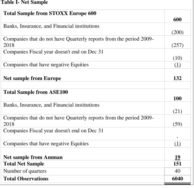
The financial variables information was collected from Thomson Returns Eikon. From it, we can get data quarterly, like stock price returns, indexes values, accounting information, and so on (Oehler, Horn, & Wendt, 2017; Achim & Tudor , 2018; Baule, 2019). We collected the economic data from the World Bank website (The world Bank, 2020). This study will use the quarterly reports between (2009-2018). The research takes a sample of companies included in the STOXX Europe 600 index and ASE100 index. It will take the companies that have the end of the fiscal year at Dec-31 to compare the liquidity of both markets during the same period, and will exclude banks, insurance, and other financial institutions since their reports have significant differences compared to the other sectors. Also, it will exclude companies that do not have quarterly financial reports available, and companies that have a negative equity amount. The ending sample consists of 151 companies from both markets as the following table:

17

Table I- Net Sample

Total Sample from STOXX Europe 600

600

Banks, Insurance, and Financial institutions

(200)

Companies that do not have Quarterly reports from the period

2009-2018

(257)

Companies Fiscal year doesn't end on Dec 31

(10)

Companies that have negative Equities

(1)

Net sample from Europe

132

Total Sample from ASE100

100

Banks, Insurance, and Financial institutions

(21)

Companies that do not have Quarterly reports from the period

2009-2018

(59)

Companies Fiscal year doesn't end on Dec 31

-

Companies that have negative Equities

(1)

Net sample from Amman

19

Total Net Sample

151

Number of quarters

40

Total Observations

6040

5- Results

5.1. Descriptive Statistics

We, firstly, show the descriptive statistics of the CFO/SALES for Jordanian and European markets.

Table II- Descriptive Statistics for STOXX EUROPE 600 and ASE100 Index in

terms of CFO/SALES

CFO/ SALES Europe CFO/SALES Jordan

Mean 0.20 0.31

Median 0.11 0.17

Maximum 20.11 96.58

Minimum -5.92 -20.40

18

Both mean and standard deviation are lower for STOXX Europe 600 than ASE100 index. We test also the equality of mean and standard deviation between the European CFO/SALES and Jordanian CFO/SALES. The Jordanian CFO/SALES has higher mean but also higher volatility comparing to the European CFO/SALES.

The mean difference is not significant but the volatility difference is significant, the results are shown in the following tables respectively, as we can see in tables III and IV.

Table II-Testing the equality of Jordanian CFO/SALES mean and European

CFO/SALES mean

Test for Equality of Means Between Series Sample: 2009Q1 2018Q4

Included observations: 760

Method df Value Probability

t-test 1518 -0.708485 0.4788

Satterthwaite-Welch t-test* 879.2182 -0.708485 0.4788

Anova F-test (1, 1518) 0.501951 0.4788

Welch F-test* (1, 879.218) 0.501951 0.4788

*Test allows for unequal cell variances

Analysis of Variance

Source of Variation df Sum of Sq. Mean Sq.

Between 1 4.484312 4.484312

Within 1518 13561.45 8.933760

Total 1519 13565.93 8.930831

Category Statistics

Std. Err.

Variable Count Mean Std. Dev. of Mean

CFO/ SALES EU 760 0.198697 1.148432 0.041658

CFO/ SALES JOD 760 0.307329 4.068000 0.147562

19

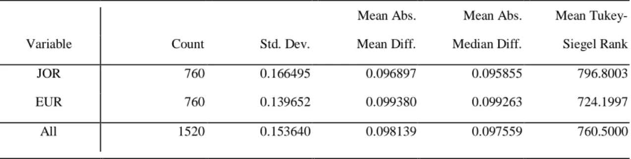
Table IIII-Testing the equality of Jordanian CFO/SALES variance and European

CFO/SALES variance

Test for Equality of Variances Between Series Sample: 2009Q1 2018Q4

Included observations: 760

Method df Value Probability

F-test (759, 759) 12.54734 * ** ***0.0000 Siegel-Tukey 12.85666 * ** ***0.0000 Bartlett 1 983.4542 * ** ***0.0000 Levene (1, 1518) 16.83130 * ** ***0.0000 Brown-Forsythe (1, 1518) 16.86515 * ** ***0.0000 Category Statistics

Mean Abs. Mean Abs. Mean Tukey- Variable Count Std. Dev. Mean Diff. Median Diff. Siegel Rank

CFO/SALES EU 760 1.148432 0.294060 0.268250 905.2268

CFO/SALES JOR 760 4.068000 0.906878 0.883197 615.7732

All 1520 2.988450 0.600469 0.575724 760.5000

Bartlett weighted standard deviation: 2.988940, *** ** and * means significance at 1%, 5%, and 10% respectively, CFO/SALES EU represents the Europe Cash Flow from Operations divided by total Sales and CFO/SALES JOR represents the Jordan Cash Flow from Operations divided by total Sales.

In the Appendix, we also provide descriptive statistics for all the variables used in our models,

5.2. Correlation matrix

From the correlation matrix in the appendix, we can see that PBV is the variable that has the highest positive correlation with both components of the stock price returns, MKTADJRET and ABNRET.

All of the correlations agree with Martani, Mulyono, & Khairurizka (2009) analysis of the effect of the financial ratios on the stock price return, except for ROE and Log TA. The increase in the firm size does not always mean a good sign for the firm, it depends on the type of the industry, and the way of managing the operational risks after the expansion (Martani, Mulyono, & Khairurizka, 2009; Singapurwoko & El-Wahid , 2011). PBV affects positively on the stock

20

price return, which agrees with Martani, Mulyono, & Khairurizka (2009), but violates other evidence like Dita & Murtaqi (2014). Considering the effect of dividends to calculate the return instead of using only the percentage change in the price, the increase in dividends will reduce both the market value and the book value of the share. However, the change in the book value is higher than the change in the market value which causes an increase in both components of the stock price return.

The increase in the market value of the stock precludes the investor to buy this stock if there was an expectation for an additional increase in the value, and when the amount collected from selling the stock later exceeds the current cost of purchasing that stock, which leads the investor to generate a profit on the long run.

By taking the absolute effect, we will notice that the CFO/SALES effect on MKTADJRET, ABNRET, and ADJ_COST is higher than the NPM effect. However, the correlations of Log TA and PBV affect more significantly on MKTADJRET and ABNRET, comparing to the other variables used in Equation 1.

5.3. Regression Analysis

We show six results of the regression analysis: firstly by showing the result of equation 1 on MKTADJRET, secondly, by showing the results of equation 1 on ABNRET, and thirdly we will show the results of analyzing equation 2 on the ADJ_COST. Also, we will rerun the two regression models by adding another two independent variables, MKT and MKT*CFO/SALES. MKT is a proxy variable to distinguish between the Jordanian market and the European market, where a value of 1 represents the Jordanian Market, while 0 represents the European Market. MKT*CFO/SALES aims to distinguish between the Jordanian Cash Flow from Operations marginal impact.

5.3.1. Market Adjusted Return (MKTADJRET)

Through Table V, we can see that the CFO/SALES will have a higher effect on the stock price over NPM, although not statistically significant. This agrees with the previous studies that CFO impacts more than earnings, and could make a change over the long-run on the stock price return (Graham & Knight, 2000; Livnat & Zarowin, 1990; Gaugha, Fuentes, & Bonanomi, 1995).

Table IV-Regression results for equation 1(MKTADJRET)

Dependent Variable: MKTADJRET Method: Panel Least Squares Sample: 2009Q1 2018Q4 Periods included: 40 Cross-sections included: 151

21

Total panel (balanced) observations: 6040

Variable Coefficient Std. Error t-Statistic Prob.

NPM 0.001043 0.001217 0.856818 0.3916 CFO/SALES 0.001948 0.001191 1.636156 0.1019 ROE -0.010156 0.010231 -0.992671 0.3209 CR -0.000319 0.001180 -0.269914 0.7872 DER 0.005024 0.002159 2.326837 * **0.0200 TATO 0.005812 0.003440 1.689675 *0.0911 PBV 0.000452 0.000227 1.988020 * **0.0469 Log TA -0.008698 0.001930 -4.507414 * ** ***0.0000 C 0.050352 0.008880 5.670289 0.0000

R-squared 0.005473 Mean dependent var 0.025724

Adjusted R-squared 0.004154 S.D. dependent var 0.143843

S.E. of regression 0.143544 Akaike info criterion -1.042860

Sum squared resid 124.2682 Schwarz criterion -1.032867

Log-likelihood 3158.438 Hannan-Quinn criter. -1.039391

F-statistic 4.148623 Durbin-Watson stat 1.831328

Prob(F-statistic) 0.000059

*** ** and * means significance at 1%, 5%, and 10% respectively.

Log TA, PBV, and DER affect significantly at 5% level comparing to other variables used in equation 1. Investors first look at the current position of the firm regarding Debt, market, and size situations, the current good situation for the firm will motivate investors to buy shares, they feel that they are in a safe position right now.

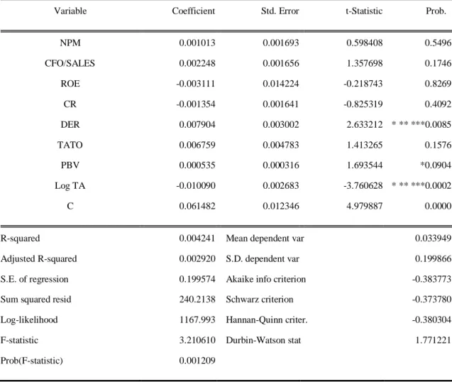
5.3.2. Cumulative Abnormal Return (ABNRET)

In table VI, we run the same regression, except that we change the measurement to ABNRET. We can notice that Log TA and DER affect more significantly on ABNRET than PBV and other variables used. Investors consider the size of the firm and the Debt situations more than the current market situations for the abnormal return, and the current market situation is first to be considered by the investors before the profitability measures.

Table V-Regression results for equation 1 (ABNRET)

Dependent Variable: ABNRET Method: Panel Least Squares

22

Sample: 2009Q1 2018Q4 Periods included: 40 Cross-sections included: 151

Total panel (balanced) observations: 6040

Variable Coefficient Std. Error t-Statistic Prob.

NPM 0.001013 0.001693 0.598408 0.5496 CFO/SALES 0.002248 0.001656 1.357698 0.1746 ROE -0.003111 0.014224 -0.218743 0.8269 CR -0.001354 0.001641 -0.825319 0.4092 DER 0.007904 0.003002 2.633212 * ** ***0.0085 TATO 0.006759 0.004783 1.413265 0.1576 PBV 0.000535 0.000316 1.693544 *0.0904 Log TA -0.010090 0.002683 -3.760628 * ** ***0.0002 C 0.061482 0.012346 4.979887 0.0000

R-squared 0.004241 Mean dependent var 0.033949

Adjusted R-squared 0.002920 S.D. dependent var 0.199866

S.E. of regression 0.199574 Akaike info criterion -0.383773

Sum squared resid 240.2138 Schwarz criterion -0.373780

Log-likelihood 1167.993 Hannan-Quinn criter. -0.380304

F-statistic 3.210610 Durbin-Watson stat 1.771221

Prob(F-statistic) 0.001209

*** ** and * means significance at 1%, 5%, and 10% respectively.

CFO/SALES has a higher effect on the ABNRET than NPM. However, the effect is also not significant. Yet, in our sample, CFO associate positively on the stock price return, and has a higher effect on both the adjusted market return and the abnormal return than N.I.

5.3.3. Adjusted Cost of Debt (ADJ_COST)

From table VII below, we can see that the CFO/SALES coefficient was -0.06%, and the absolute negative coefficient was higher than the absolute negative coefficient of NPM. In this model, the effect of CFO/SALES was significant at 5% level.

Table VIII-Regression Analysis for equation 2

Dependent Variable: ADJ_COST Method: Panel Least Squares

23

Sample: 2009Q1 2018Q4 Periods included: 40 Cross-sections included: 151

Total panel (balanced) observations: 6040

Variable Coefficient Std. Error t-Statistic Prob.

NPM -0.000458 0.002673 -0.171389 0.8639 CFO/SALES -0.006070 0.002604 -2.331101 * **0.0198 LEV 0.285425 0.032429 8.801515 * ** ***0.0000 EBIT/INT -0.000324 1.60E-05 -20.25253 * ** ***0.0000 MAT 0.216277 0.016615 13.01670 * ** ***0.0000 PROF -0.153041 0.198277 -0.771853 0.4402 TANG 0.035240 0.022281 1.581586 0.1138 SIZE 0.085270 0.005411 15.75971 * ** ***0.0000 MTB -0.001676 0.003685 -0.454692 0.6493 INF -0.005323 0.003289 -1.618331 0.1056 R_LAW -0.014386 0.013768 -1.044901 0.2961 LEG_IND -0.024801 0.007641 -3.245680 * ** ***0.0012 DEP_INF -0.053427 0.007668 -6.967248 * ** ***0.0000 DEP_INF*LEG_IND 0.009523 0.001463 6.511639 * ** ***0.0000 B_CREDIT -0.002232 0.000158 -14.16266 * ** ***0.0000 B_CONC 0.002132 0.000495 4.310751 * ** ***0.0000 C 0.598765 0.037430 15.99677 0.0000

R-squared 0.229269 Mean dependent var 0.851159

Adjusted R-squared 0.227221 S.D. dependent var 0.355961

S.E. of regression 0.312918 Akaike info criterion 0.517058

Sum squared resid 589.7574 Schwarz criterion 0.535933

Log-likelihood -1544.516 Hannan-Quinn criter. 0.523611

F-statistic 111.9784 Durbin-Watson stat 0.622683

Prob(F-statistic) 0.000000

*** ** and * means significance at 1%, 5%, and 10% respectively.

The economic variables of each country play also an important role, like the firm's variables, in explaining the cost of Debt. The stronger the regulations and the protection of the lenders, the more it will reduce the cost of Debt charged to the firm (Alvarez-Botas & Gonzalez, 2019; Bae

24

& Goyal, 2009; Qian, Cao, & Cao, 2018), and more information available for the lenders about the borrower will make them charge a lower cost (Quijano, 2013; Beladi & Quijano, 2013; Petersen & Rajan, 1994).

However, by looking at table XIX (see appendix VI), the correlation between the R_LAW and the interaction of R_LAW*LEG_IND was 0.93, which is closer to 1, to deal with the Multicollinearity we run the regression model excluding R_LAW*LEG_IND. The result are shown in Table IV below. CFO/SALES is significant at 5%, while the NPM is not significant.

Both NPM and CFO/SALES affect negatively on the cost of Debt, but the CFO/SALES effect is more significant. CFO associates negatively on the Cost of Debt, by reducing it, and it has a higher absolute effect comparing to the N.I.

Our findings to the main research question is that CFO, as a component of earnings, does matter both for Stock and Debt holders. Both N.I and CFO are relevant components of earnings in explaining the movements of the market-adjusted return and the cumulative abnormal return. However, CFO has a higher impact for Debt holders than N.I. CFO has a higher effect than N.I on both the stock price returns and the cost of debt. Results are still not significant for stock price returns. Regarding the cost of Debt, the effect of CFO is significant because the holders of the debt would charge the firm a commission for delaying the payments of the accrued debt or interest, the bankers will require more return on their loans because the maturity of banks Assets are less than the maturity of banks liabilities, meaning that the amount of interests received is less than the interests paid compared to the same time, so the demand of money by the borrowers will be charged with a higher cost for the firms that has a weak CFO amount (Gambacorta & Mistrulli, 2004). In general, this may indicate that the effect of CFO depends on the investment horizon.

5.4. Comparing the liquidity between STOXX Europe 600 and ASE100 indexes

As mentioned in section, we will add another two independent variables to the equations 1 and 2 to compare between the European market and the Jordanian market. MKT is a variable that receives a value of 1 if the firm is Jordanian, and 0 if the firm is European, and MKT*CFO/SALES to distinguish between the European CFO/SALES and Jordanian CFO/SALES.

Table VII-testing the effect of MKT and MKT*CFO/SALES on MKTADJRET

Dependent Variable: MARADJRET Method: Panel Least Squares Sample: 2009Q1 2018Q4 Periods included: 40 Cross-sections included: 151

25

Variable Coefficient Std. Error t-Statistic Prob.

NPM 0.000486 0.001304 0.372513 0.7095 CFO/SALES 0.003510 0.002894 1.213081 0.2251 ROE -0.015765 0.010245 -1.538730 0.1239 CR -0.000225 0.001178 -0.191304 0.8483 DER 0.004922 0.002153 2.286410 * **0.0223 TATO 0.002795 0.003480 0.803371 0.4218 PBV 0.000336 0.000228 1.476945 0.1397 Log TA -0.019793 0.002659 -7.445310 * ** ***0.0000 MKT -0.049051 0.008148 -6.020152 * ** ***0.0000 MKT*CFO/SALES -0.002044 0.003302 -0.619063 0.5359 C 0.101944 0.012391 8.227275 0.0000

R-squared 0.011666 Mean dependent var 0.025724

Adjusted R-squared 0.010026 S.D. dependent var 0.143843

S.E. of regression 0.143120 Akaike info criterion -1.048444

Sum squared resid 123.4944 Schwarz criterion -1.036231

Log likelihood 3177.301 Hannan-Quinn criter. -1.044204

F-statistic 7.116153 Durbin-Watson stat 1.842522

Prob(F-statistic) 0.000000

*** ** and * means significance at 1%, 5%, and 10% respectively.

From table VIII, we can notice that MKT is significant, and has a negative effect on the MKTADJRET, and MKT*CFO/SALES affect negatively on MKTADJRET. This means that the European Market Adjusted Return is higher than the Jordanian Market Adjusted Return, and the CFO for the European market increases the MKTADJRET more than the CFO for the Jordanian market. However, the effect of MKT*CFO/SALES is not significant.

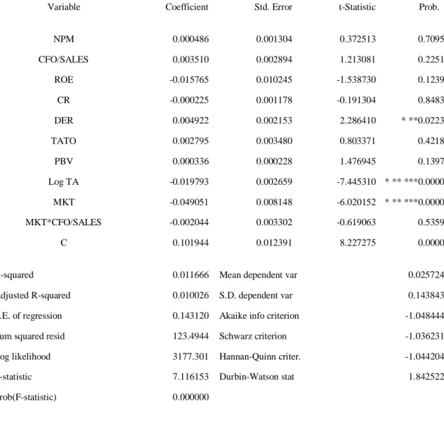
Table VIII- testing the effect of MKT and MKT*CFO/SALES on ABNRET

Dependent Variable: ABNRET Method: Panel Least Squares Sample: 2009Q1 2018Q4 Periods included: 40 Cross-sections included: 151

26

Variable Coefficient Std. Error t-Statistic Prob.

NPM 0.001441 0.001812 0.795465 0.4264 CFO/SALES -0.002486 0.004020 -0.618323 0.5364 ROE -0.012261 0.014233 -0.861445 0.3890 CR -0.001361 0.001636 -0.831749 0.4056 DER 0.007754 0.002991 2.592626 * ** ***0.0095 TATO 0.001387 0.004834 0.286922 0.7742 PBV 0.000361 0.000316 1.141011 0.2539 Log TA -0.027531 0.003693 -7.454285 * ** ***0.0000 MKT -0.077634 0.011319 -6.858593 * ** ***0.0000 MKT*CFO/SALES 0.005786 0.004588 1.261126 0.2073 C 0.144316 0.017214 8.383644 0.0000

R-squared 0.012002 Mean dependent var 0.033949

Adjusted R-squared 0.010363 S.D. dependent var 0.199866

S.E. of regression 0.198828 Akaike info criterion -0.390935

Sum squared resid 238.3415 Schwarz criterion -0.378722

Log-likelihood 1191.624 Hannan-Quinn criter. -0.386695

F-statistic 7.323859 Durbin-Watson stat 1.784247

Prob(F-statistic) 0.000000

*** ** and * means significance at 1%, 5%, and 10% respectively.

From table IX, we can notice that MKT is significant, and has a negative effect on the ABNRET, and MKT*CFO/SALES affect positively on ABNRET. This means that the European Cumulative Abnormal Return is higher than the Jordanian Cumulative Abnormal Return, but the CFO for the Jordanian market increases the ABNRET more than the CFO for the European market, and the effect of CFO/SALES turned to be negative on the Abnormal Return by adding the two independent variables MKT and MKT*CFO/SALES to the regression. However, each effect of MKT*CFO/SALES and CFO/SALES itself is insignificant.

Table IX- testing the effect of MKT and MKT*CFO/SALES on Cost of Debt

Dependent Variable: ADJ_COST Method: Panel Least Squares Sample: 2009Q1 2018Q4 Periods included: 40 Cross-sections included: 151