Clock Synchronization for Moderm Multiprocessors

(1)

CLOCK SYNCHRONIZATION FOR

MODERN MULTIPROCESSORS

ANDRÉ DOS SANTOS OLIVEIRA

DISSERTAÇÃO DE MESTRADO APRESENTADA

À FACULDADE DE ENGENHARIA DA UNIVERSIDADE DO PORTO EM ENGENHARIA ELETROTÉCNICA E DE COMPUTADORES

(2)

(3)

F

ACULDADE DE

E

NGENHARIA DA

U

NIVERSIDADE DO

P

ORTO

Clock Synchronization for Modern

Multiprocessors

André dos Santos Oliveira

Mestrado Integrado em Engenharia Eletrotécnica e de Computadores Supervisor: Pedro Alexandre Guimarães Lobo Ferreira Souto

(4)

(5)

Abstract

Multi-corearchitectures, in which multiple processors (cores) communicate directly through shared hardware to performs parallel tasks and that way increasing the execution performance, are becom-ing very present in computer systems, and are increasbecom-ingly relevant in Real-Time (RT) applica-tions, from data-centers to embedded-systems, not to mention desktops. Clock synchronization is a critical service on many of these systems.

This dissertation focuses on clocks in synchronous digital systems, in particular Intel architec-tures, from the distribution and analysis of the clock signal in order to coordinate data paths, to software methods and hardware interactions to maintain a time base accurately across a plurality of interconnected processors with possibly different notions of time.

In addition, a clock synchronization algorithm in a shared-memory multi-core architectures is proposed, as if it’s a distributed system, applying a model to filter outlet samples, resulting in a random process that achieves a null offset after a couple of corrections. Some experimental measures were made as well to characterize the speed reading the clock and the communication methods used between different cores.

(6)

(7)

Resumo

As arquiteturas multi-core, em que múltiplos processadores (cores) cooperam entre si através de hardware partilhado para realizar tarefas paralelas e assim aumentar a performance de execução, são cada vez mais presentes nos sistemas computacionais, e cada vez mais relevantes em apli-cações de tempo real, desde em centros de dados a sistemas embarcados, para não falar dos desk-tops. A sincronização de relógios é um serviço crucial em muitos destes sistemas.

Esta dissertação concentra-se em relógios de sistemas digitais síncronos, em particular arquite-turas multi-core, desde a distribuição e análise do sinal de relógio para coordenar as interfaces de dados, a métodos de software e interações com o hardware para manter uma base de tempo precisa e síncrona numa pluralidade de processadores interligados com possivelmente diferentes noções de tempo.

Para além disso, é proposto um algoritmo de sincronização de relógios em sistemas multi-core com memória partilhada, como se de um sistema distribuído se tratasse, aplicando um modelo de filtragem de falsas amostras de tempo, resultando num processo aleatorio que coloca o offset nulo após algumas correções. Foram também feitas algumas medidas experimentais para caracterizar a velocidade de leitura do relógio e os mecanismos usados de comunicação entre diferentes cores.

(8)

(9)

Acknowledgments

Esta dissertação representa o culminar de um percurso académico de trabalho, aprendizagem, e crescimento pessoal junto de pessoas inspiradoras.

Quero agradecer ao meu orientador, Pedro Ferreira Do Souto, pela motivação que me deu nos momentos de maior dificuldade e insegurança, pelo espirito desafiador nos momentos de maior confiança, e pela paciência que teve comigo na focalização do que era essencial.

À equipa técnica do CISTER, por me acolher nas suas instalações e me fornecer material, em especial ao professor Paulo Baltarejo Sousa (DEI-ISEP) por ser uma das únicas pessoas a quem podia recorrer em momentos dificeis, dada a elevada especificidade desta dissertação, e por toda a ajuda que me deu.

A todos os professores que tive oportunidade de conhecer e trabalhar na licenciatura no ISEP, e no mestrado na FEUP, que me formaram e me moldaram para me tornar aquilo que sou hoje, e o Engenheiro que serei no futuro.

Quero agradecer a toda a minha família, em especial aos meus pais, por tudo o que me propor-cionaram, pela confiança que sempre tiveram nas minhas capacidades, pela motivação e inspiração que me deram nos momentos mais difíceis deste percurso, e pela paciência que tiveram a lidar comigo e com as minhas atitudes às vezes injustas. Tudo o que sou deve-se ao que me ensinaram e mostraram ao longo da vida.

E por ultimo mas não menos importante, a todos os meus amigos que partilharam comigo este percurso, e me incentivaram a saber mais e aprender mais, e me ensinaram a importância de trabalhar em equipa, em especial aos meus companheiros de mestrado Pedro Medeiros, Luís Duarte, João Lima e André Sá, assim como às pessoas que me acompanharam na fase final, em especial à Fátima Airosa, que me deram a motivação que tanto precisei e a força para manter a confiança necessária à conclusão desta etapa com sucesso. Também devo tudo isto aos meus amigos de longa data que estiveram sempre presentes e pelos momentos inesquecíveis que vivemos e que vão sempre definir parte da minha pessoa.

André Oliveira

(10)

(11)

”A man with a watch knows what time it is. A man with two watches is never sure”

Segal’s law

(12)

(13)

List of Figures

2.1 Local Data Path . . . 6

2.2 Positive and Negative clock Skew . . . 7

2.3 Variations on the balanced tree topology . . . 10

2.4 Central clock spine distribution . . . 10

2.5 Clock grid with 2-dimensional clock drivers . . . 11

2.6 Asymmetric clock tree distribution . . . 11

2.7 Globally synchronous and locally synchronous architecture . . . 13

2.8 Data structures for managing timers . . . 19

2.9 Overview of the generic time subsystem . . . 20

2.10 The relation between clock time and UT when clocks tick at different rates . . . . 27

2.11 Getting the current time from a time server. . . 28

2.12 The Berkeley Algorithm . . . 29

2.13 PTP message exchange diagram [tutorial] . . . 30

3.1 CPUID raw output data . . . 34

3.2 Initial available clock sources . . . 35

3.3 Make menuconfig interface . . . 37

3.4 Results from experiments on read latency . . . 40

4.1 Synchronization method with IPIs . . . 45

4.2 Synchronization method with cache coherency . . . 47

4.3 IPI latency experiment results . . . 48

4.4 Cache Coherence latency experiment results . . . 48

4.5 Flowchart of DAC model . . . 49

5.1 Cache Coherence synchronization method results . . . 57

(16)

(17)

List of Tables

2.1 Clock distribution topologies . . . 9

2.2 Clock distribution characteristics of commercial processors. . . 12

2.3 Clock synchronization categories . . . 12

(18)

(19)

Abbreviations and Symbols

ACPI Advanced Configuration and Power Interface API Application Programming Interface

APIC Advanced Programmable Interrupt Controller CMOS Complementary Metal Oxide Semiconductor CPU Central Processing Unit

DAC Delay Asymmetry Correction EOI End-Of-Interrupt

FLOPS FLoating-point Operations Per Second FTA Fault-Tolerant Average

GALS Globally Asynchronous Locally Synchronous HPET High Precision Event Timer

HRT High Resolution Timer IC Integrated circuit

ICR Interrupt Command Register IPI Inter-Processor Interrupt IRQ Interrupt Request

IRR Interrupt Request Register ISR In-Service Register KILL Kill If Less than Linear LKM Loadable Kernel Module LVT Local Vector Table MIC Many Integrated Core

MPCP Multiprocessor Priority Ceiling Protocol MSR Model Specific Register

NOC Network On Chip NTP Network Time Protocol PC Personal Computer

PIT Programmable Interrupt Timer PLL Phase-Locked Loop

PM Power Management PTP Precision Time Protocol POD Point-Of-Divergence

RBS Reference Broadcast Synchronization

RT Real-Time

RTC Real Time Clock RTL Register-Transfer Level SCA Synchronous Clocking Area SMP Symmetric Multiprocessor System

(20)

SOC System On Chip

SRP Stack-based Resource Policy TAI International Atomic Time TSC Time Stamp Counter UTC Universal Time Coordinated VLSI Very Large Scale Integration

(21)

Chapter 1

Introduction

1.1 Contextualisation

The use of computer systems is greatly increasing in real-time applications. In these systems, the operations performed must deliver results on time, otherwise we may have effects of quality re-duction, or even disastrous. So the time that operations take to run need to be controlled effectively in the design of real-time systems.

In order to introduce parallelism in performing tasks, the concept of multicore/multiprocessor was born, a computer system that contains two or more processing units that share memory and peripherals to process simultaneously. These systems are increasingly relevant in real-time (RT) applications and clock synchronization is a critical service on many of these systems, as the lack of synchronization between the multiple cores can for example degrade the quality of the scheduling algorithms that rely on cooperation.

1.2 The problem, Motivation and Goals

Clock synchronization is commonly assumed as a given or even to be perfect in multiprocessor platforms. In reality, even in systems with a shared clock source, there is an upper bound on the precision with which clocks can be read on different processors. If we are to take advantage of a clock service in a real-time system on a multi-processor platform, it is critical to be able to quantify the quality of that service.

This dissertation has the main purpose of estimating the quality of a clock service provided by Linux on common-of-the-shelf multi-core processors such as those of the x64 architectures, and if possible to design and implement a clock synchronization algorithm that would minimize the clock differences, characterizing its implications and limitations.

As an example of the advantage of having access to a synchronized clock in a multi-core system, we describe next its application to a hard real-time semi-partitioned scheduling algorithm for multiprocessors.

(22)

In hard real-time systems, application processes, usually referred to as tasks in the literature, can be analysed as if they were periodic. The execution of such processes in each period is often denoted as a job. A critical aspect in a hard-real time system is to ensure that each job of a process is executed before its deadline, which is assumed to be known at design time. Therefore it is essential that the system uses an appropriate scheduling algorithm, allocating cores to each job.

A class of hard real-time scheduling algorithms is known as semi-partitioned. In these algo-rithms, some jobs may migrate from one core to another to improve core utilization. Therefore, the execution of a migrating job may be described as a sequence of sub-jobs executing in different cores. This means that a sub-job, which is allocated to one core, may not execute before the pre-vious sub-job, which executes on another core, terminates. These precedence constraints can be satisfied by releasing a sub-job only after the previous sub-job has completed.

A straightforward way to do that is to use some inter-processor communication mechanism, such as the inter-processor interrupt (IPI) on the Intel 64 and IA-32 architectures. I.e. when a sub-job terminates, the scheduler running on the same core may generate an IPI to the core that will run the next sub-job. The handling of this IPI will release the next sub-job, which will eventually be scheduled. The problem with this approach is that this communication is on the critical path, with respect to the response time, and, because IPIs are sent via shared bus, the delays incurred may be rather large. Because in hard-real time one must ensure that deadlines are satisfied, usually by carrying out a timing analysis, this implementation may lead to an overly pessimistic estimation of the job response time and therefore to a low CPU utilization.

By relying on high-resolution timers, i.e. timers that are able to measure time with a resolution of 1 microsecond or better, one can reduce the overhead caused by all IPIs but the first. The idea is as follows. Through a timing analysis it is possible to determine the latest time, relative to its release, at which each sub-job will complete. Therefore, one way to ensure the precedence constraints of the different jobs is to schedule the release of each sub-job to the earliest time one can ensure the previous sub-job will be completed. One possible implementation of this approach is as follows: upon release of a migrating job, the scheduler on the core where this happens, will send an IPI to each of the cores that execute the other sub-jobs of that job. The handler of this IPI in each of the cores will then program a high-resolution timer to release the sub-job to a time by which the previous sub-job has terminated. The value with which each high-resolution timer is programmed, must take into account the variability of response time to IPIs. As mentioned earlier, IPIs are sent via a shared bus, which may delay the sending of the IPI. In addition, at each core, received IPIs may be queued behind other interrupts. So, again, this may lead to some pessimism. One way to reduce further this pessimism is to use synchronized clocks. If each core has access to a global high-resolution clock, the core where the first sub-job is released may timestamp that event, and send an IPI to all cores where the other sub-jobs will be executed. Upon receiving this IPI, the release time of the first sub-job can be read rather than estimated. Therefore in the programming of the high resolution timers used to release the different sub-jobs, rather than using the maximum IPI delay, one can use the actual delay in the delivery of the IPI. In terms of the timing analysis, the IPI delay and its jitter is not in the critical path anymore. Instead, we need to

(23)

1.3 Document Structure 3

take into account the accuracy of the clock readings at the different cores.

This algorithm has triggered this research work, but we believe that clock synchronization can be used in other scheduling algorithms, as well as in other resource management algorithms.

1.3 Document Structure

In addition to the introduction, this dissertation has 5 more chapters. Chapter2presents a review of the state of the art, focusing on the theoretical background necessary to understand the concepts in the scope of this dissertation. Chapter3states the description of the clock to be later synchronized as well as its implications, and chapter 4 shows how to synchronize these clocks. Chapter 5

describes the data export mechanism and an analysis on the results of the experiments carried out, and finally chapter 6 presents the final appreciations on the work as well as improvement suggestions to be made in the future.

(24)

(25)

Chapter 2

State of the art

This chapter presents some relevant state-of-art information related to the hardware trends in clock distribution networks in integrated circuits, the operating system time services that keep track of time, and some clock synchronization algorithms present in today’s distributed systems.

2.1 Clock Source Distribution

In this section, a review on the clock signal distribution technologies is presented, in order to understand the relevant parameters in a characterization of the clocks.

2.1.1 Introduction

The clock signal is used to define a time reference for the movement of data within a synchronous digital system, hence it is a vital signal to its operation [1].

Utilized like a metronome to coordinate actions, this signal oscillates between a high and a low state, typically loaded with the greatest fanout, travel over the longest distances, and operate at the highest speeds of any signal.

The data signals are provided and sampled with a temporal reference by the clock signals, so the clock waveforms must be particularly clean and sharp, and any differences in the delay of these signals must be controlled in order to limit as little as possible the maximum performance as well as to not create catastrophic race condition in which an incorrect data signal propagates within a register (latch or flip-flop).

In order to address these design challenges successfully, it is necessary to understand the fun-damental clocking requirements, key design parameters that affect clock performance, different clock distribution topologies and their trade-offs, and design techniques needed to overcome cer-tain limitations.

(26)

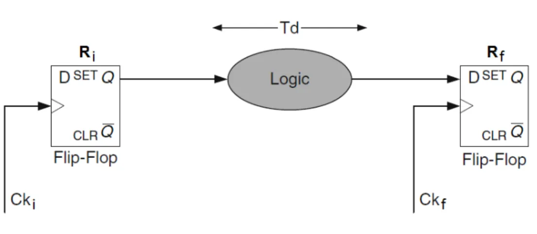
Figure 2.1: Local Data Path

2.1.2 Synchronous Systems

A digital synchronous circuit is composed of a network of functional logic elements and globally clocked registers.

If an arbitrary pair of registers are connected by at least one sequence of logic elements, a switch event at the output of R1 will propagate to the input of R2. In this case, (R1,R2) is called a

sequentially-adjacent pair of registers which make up a local data path.

An example of a local data path Ri- Rf is shown in figure2.1. The clock signals Ckiand Ckf

synchronize the sequentially-adjacent pair of registers Riand Rf, respectively. Signal switching at

the output of Ri is triggered by the arrival of the clock signal Cki, and after propagating through

the Logic block, this signal will appear at the input of Rf.

In order to the switch of the output of Ri to be sampled properly in the input of Rf in the

next clock period, data path has to have time to stabilize the result of the combinational logic in the input of Rf, so the minimum allowable clock period TCP(min) between any two registers in a

sequential data path is given by equation2.1. 1

fclkMAX

= TPD(max)+ TSkewi f (2.1) where fclkMAX is the maximum clock frequency, and TPD(max)= TC−Q+ Td+ Tint+ Tsetup.

The total path delay of the data path TPD(max)is the sum of the maximum propagation delay of

the flip-flop, TC−Q, the time necessary to propagate through the logic and interconnect, Td + Tint,

and the setup time of the output flip-flop, Tsetup, which is the time that the data to be latched must

be stable before the clock transition.

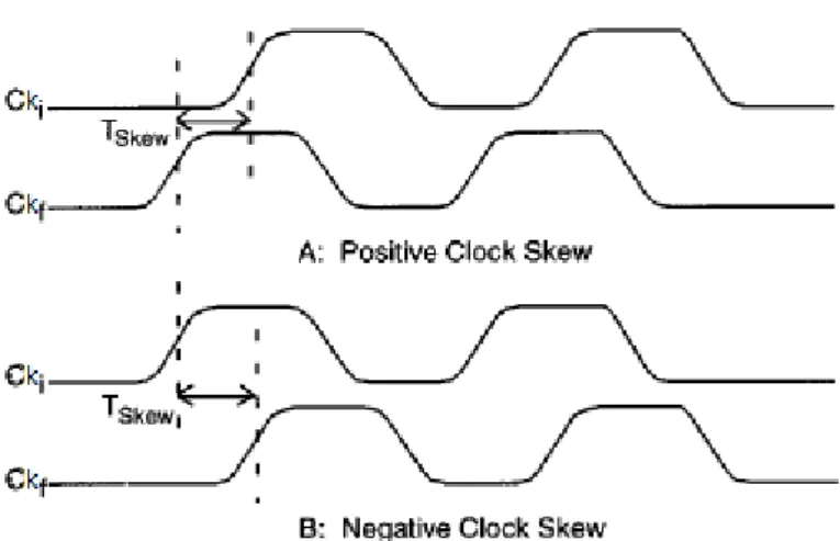
The clock skew TSkewi f can be positive or negative depending on whether Ckilags or leads Ckf, respectively, as shown in figure2.2.

(27)

2.1 Clock Source Distribution 7

Figure 2.2: Positive and Negative clock Skew

2.1.3 Clock Skew

The propagation delay from the clock source to the jth clocked register is the clock delay, Ckj.

The clock delays of the initial clock signal Ckiand the final clock signal Ckf define the time

reference when the data signals begin to leave their respective registers.

The difference in clock signal arrival time (clock delay from the clock source) between two sequentially-adjacent registers Riand Rf is called Clock Skew.

The temporal skew between different clock signal arrival times is only relevant to sequentially-adjacent registers making up a single data path, as shown in figure2.1. Thus, system-wide (or chip-wide) clock skew between non-sequentially connected registers, from an analysis viewpoint, has no effect on the performance and reliability of the synchronous system.

Synchronous circuits may be simplified to have two timing limitations: setup (MAX delay) and hold (MIN delay) [2].

Setupspecifies whether the digital signal from one stage of the sequential structure has suffi-cient time to travel and set up before being captured by the next stage of the sequential structure.

Holdspecifies whether the digital signal from the current state within a sequential structure is immune from contamination by a signal from a future state due to a fast path.

The setup constraint specifies how data from the source sequential stage at cycle N can be captured reliably at the destination sequential stage at cycle N+1.

The constraint for the source data to be reliably received is defined by equation2.2.

Tper≥ Td−slow+ Tsu+ | TCk1− TCk2| (2.2)

where Tper is the clock period, Td−slowis the slowest (maximum) data path delay, Tsuis the setup

time for the receiver flip-flop, TCk1and TCk2are the arrival times for clocks Ck1and Ck2(at cycle

N) respectively.

In this situation, the available time for data propagation is reduced by the clock uncertainty defined as the absolute difference of the clock arrival times.

(28)

In order to meet the inequality, either clock period must be extended or path delay must be reduced. In either case, power and operating frequency may be affected.

The hold constraint specifies the situation where the data propagation delay is fast, and clock uncertainty makes the problem even worse and the data intended to be captured at cycle N +1 is erroneously captured at cycle N, corrupting the receiver state.

In order to ensure that the hold constraint is not violated, the design has to guarantee that the minimum data propagation delay is sufficiently long to satisfy the inequality 2.3, where Thold is

the hold time requirement for the receive flip-flop.

Td− f ast≥ Thold+ | TCk1− TCk2| (2.3)

In sum, the relationship in2.4is expected to hold.

Td− f ast< Td−nominal< Td−slow (2.4)

Localized clock skew can be used to improve synchronous performance by providing more time for the critical worst case data paths.

By forcing Ck1 to lead Ck2 at each critical local data path, excess time is shifted from the

neighboring less critical local data paths to the critical local data paths.

Negative clock skew subtracts from the logic path delay, thereby decreasing the minimum clock period. Thus, applying negative clock skew, in effect, increases the total time that a given critical data path has to accomplish its functional requirements by giving the data signal released from Rimore time to propagate.

2.1.4 Clock Distribution Network Topologies

Distributing a tightly controlled clock signal within specific temporal bounds is difficult and prob-lematic.

The design methodology and structural topology of the clock distribution network should be considered in the development of a system for distributing the clock signals. Furthermore, the trade-offs that exist among system speed, physical die area, and power dissipation are greatly af-fected by the clock distribution network. Intentional or unintentional structural design mismatches could lead to clock uncertainties, which can be corrected by careful pre-silicon analysis and design or post-silicon adaptive compensation techniques. Therefore, various clock distribution strategies have been developed over the years.

The trend nowadays is to the adoption of clock distribution topologies that are skew tolerant, more robust design flow, and the incorporation of robust post-silicon compensation techniques, as well as multi-clock domain distributions, with the concept of design called GALS (Globally Asynchronous and Locally Synchronous).

(29)

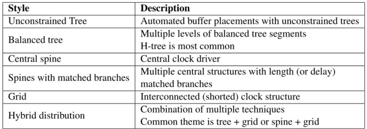
Table 2.1: Clock distribution topologies

Style Description

Unconstrained Tree Automated buffer placements with unconstrained trees Balanced tree Multiple levels of balanced tree segments

H-tree is most common Central spine Central clock driver

Spines with matched branches Multiple central structures with length (or delay) matched branches

Grid Interconnected (shorted) clock structure

Hybrid distribution Combination of multiple techniques

Common theme is tree + grid or spine + grid

2.1.4.1 Unconstrained Tree

A very common strategy for distributing clock signals used in the history of VLSI (Very Large Scale Integration) systems was to insert buffers at the clock source and along a clock path, forming a tree structure.

The clock source is frequently described as the root of the tree, the initial portion of the tree as the trunk, individual paths driving each register as the branches, and the registers being driven as the leaves. The distributed buffers serve the double function of amplifying the clock signals degraded and isolating the local clock nets from upstream load impedances.

In the unconstrained tree clock network, there is little or none constraints imposed on the network’s geometry, number of buffers or wire lengths. It is typically accomplished by automatic RTL (Register Transfer Level) synthesis flow tools with a cost heuristic algorithm that minimizes the delay differences across all clock branches.

But due to limitations regarding process parameter variations, this style is usually used for small blocks within large designs.

2.1.4.2 Balanced Trees

Another approach is to use a structural symmetric tree with identical distributed interconnect and buffers from the root of the distribution to all branches. This design ensures zero structural skew, hence the delay differences among the signal paths is due to variations of the process parameters.

Figure2.3shows alternative balanced tree topologies: the tapered X-tree, the H-tree and the binary tree. In a tapered H-tree, the trunk are designed to be wider towards the root of the distri-bution network to maintain impedance matching at the T-junctions, as it can be seen in the figure. These three topologies, called Full balanced tree topologies are designed to span the entire die in both the horizontal and vertical dimensions. Binary tree on the other hand is intended to deliver the clock in a balanced manner in either the vertical or horizontal dimension.

Since the buffers in a binary tree are physically closer to each other, resulting in a reduced sensitivity to on-die variations, and H-tree and X-tree clock distribution networks are difficult to

(30)

Figure 2.3: Variations on the balanced tree topology (left) X-tree; (center) H-tree; (right) Binary tree;

achieve in VLSI-based systems which are irregular in nature, binary trees are often the preferred structure over an idealized H-tree.

2.1.4.3 Central Spines

A central spine clock distribution is a specific implementation of a binary tree.

The binary tree is shown to have embedded shorting at all distribution levels and unconstrained routing to the local loads at the final branches. In this configuration, the clock can be transported in a balanced fashion across one dimension of the die with low structural skew. The unconstrained branches are simple to implement although there will be residual skew due to asymmetry, as the figure2.4shows.

Multiple central spines can be placed to overcome this issue, dividing the chip into several sectors to ensure small local branch delays.

Figure 2.4: Central clock spine distribution

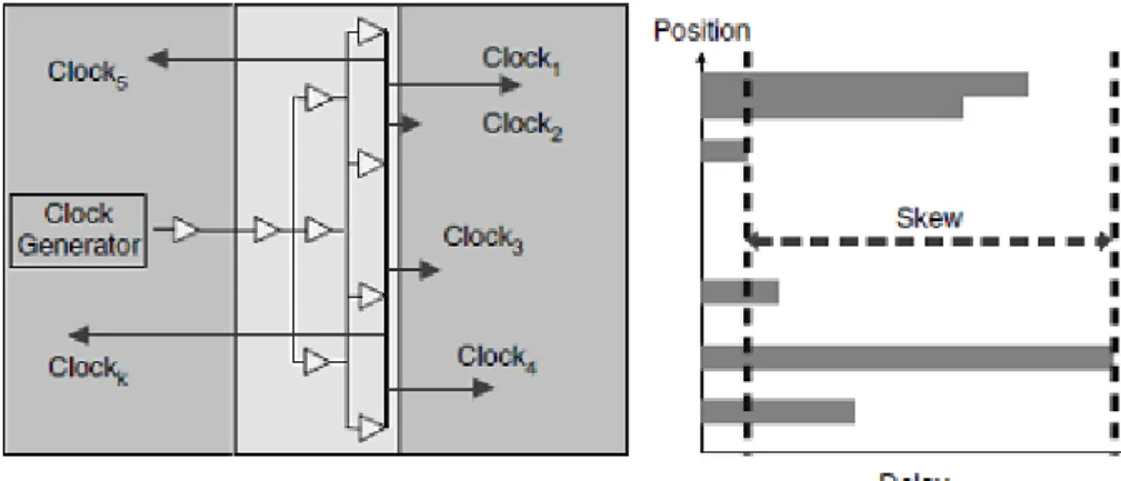
2.1.4.4 Grid

A processor will have a large number of individual branches to deliver the clock to the local points, and therefore a deep distribution tree is needed, degrading the clock performance. A superior solution can be subdividing the die into smaller clock regions and applying a grid to serve each

(31)

region. The grid effectively shorts the output of all drivers and helps minimize delay mismatches, resulting in a more gradual delay profile across the region.

Figure 2.5: Clock grid with 2-dimensional clock drivers

2.1.4.5 Hybrid Distribution

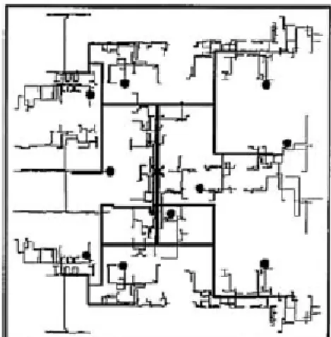
In a processor design, the most common design technique is the hybrid clock distribution. It incorporates a combination of other topologies, providing more scalability. A common approach is the tree-grid distribution, that employs a multi-level H-tree driving a common grid that includes all local loads. Figure2.6 shows an example of a processor clock distribution with a first level H-tree connected to multiple secondary trees that are asymmetric but delay balanced.

Several clock distribution topologies have been presented. The primary objective is to deliver the clock to all corners of the die with low skew. Possible improvements of the original tree distribution system consist in providing the clock generator with a skew compensation mechanism [3].

Even if the adaptive design may exhibit higher initial skew, the physical design resource needs for a clock network with adaptive compensation are expected to be lower, because of the need for accurate and exhaustive analysis for all process effects

(32)

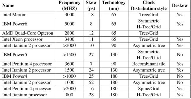
The evolution of the processor clock distribution designs eventually incorporated adaptive clock compensation. The table 2.2 [2] summarizes clock distribution characteristics of various commercial processors.

Table 2.2: Clock distribution characteristics of commercial processors.

Name Frequency (MHZ) Skew (ps) Technology (nm) Clock

Distribution style Deskew

Intel Merom 3000 18 65 Tree/Grid Yes

IBM Power6 5000 8 65 Symmetric

H-Tree/Grid Yes

AMD Quad-Core Opteron 2800 12 65 Tree/Grid

Intel Xeon processor 3400 11 65 Tree/Grid Yes

Intel Itanium 2 processor >2000 10 90 Asymmetric tree Yes

IBM Power5 >1500 27 130 Symmetric

H-Tree/Grid No

Intel Pentium 4 processor 3600 7 90 Recombinant tile Yes

Intel Itanium 2 processor 1500 24 130 Asymmetric tree Yes

IBM Power4 >1000 25 180 Tree/Grid No

Intel Itanium 2 processor 1000 52 180 Asymmetric tree No

Intel Pentium 4 processor >2000 16 180 Spine/Grid Yes

Intel Itanium processor 800 28 180 H-Tree/Grid Yes

2.1.5 Multiclock Domain and Parallel Circuits

As technology scaling comes closer to the fundamental laws of physics, the problems associated with technology and frequency scaling become more and more severe. Technology and frequency scaling alone can no longer keep up with the demand for better CPU performance [4].

In addition, the failure rate in the generation of a global clock began to raise concerns about the dependability of the future VLSI chips [5]. To overcome this problem, VLSI chips came to be regarded not as a monolithic block of synchronous hardware, where all state transitions occur simultaneously, but as a large digital chip partitioned into local clock areas, each area operating synchronously and served by independent clocks within the domain, that can be multiple copies

Table 2.3: Clock synchronization categories Type Characteristics of distribution

Synchronous Single distribution point-of-divergence (POD) with known static delay offsets among all the branches and single operating frequency. Mesochronous Single distribution POD but with nonconstant delay offset among

the branches.

Plesiochronous Multiple distribution PODs but with nominally identical frequency among all the domains.

Heterochronous Multiple distribution PODs with nominally different operating frequencies among the domains.

(33)

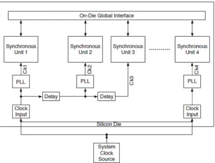
of the system clock, at different phases or frequencies. These areas are also known as isochronous zones or synchronous clocking areas (SCAs). Dedicated on-die global interfaces are needed to manage data transfer among the domains.

As digital designs move towards multicore and SOC (Systems-on-Chip) architectures, this concept of multiple clock domains have become a prevalent design style, and the clock distribution schemes will need to be enhanced to fulfill this need. Each synchronous unit will rely on any of the conventional clock distribution topologies described before to achieve low skew and fully synchronous operation.

This scheme provides functional flexibility for each of the domains to operate at a lower fre-quency than a single-core processor and to minimize the complexity and power associated with global synchronization.

The multidomain clock distribution architectures for multicore processors and SoCs belong to a GALS class of designs. Table2.3summarizes synchronization categories within the GALS class and figure2.7shows a generic illustration of the GALS design style.

A plesiochronous clock distribution example is the 65nm dual core Xeon processor, wich con-sists of two domains for the two cores and the uncore and I/O domain with the interface operating at the same frequency. It uses three independent distribution PODs for the cores and the uncore.

An example of mesochronous clocking cheme, i.e. using the same frequency but with un-known phase [6], is the NoC (Network-on-Chip) teraFLOPS processor. [7]

The 90nm 2-core Itanium and the 65nm quad-core Itanium processors are examples of a het-erochronous clock distribution, supporting nominally different operating frequencies across the domains with multiple clock generators, i.e. PLLs .

Many modern multicore processors and SoCs only adopt the loosely synchronous styles of the

(34)

above to avoid the significant complexity associated with truly asynchronous design, which is an intrinsically analog system, since the time is continuous, and the risk of metastability because the clocks of SCAs that are not really fully independent, is not negligible.

For these reasons, reliability is difficult to guarantee in truly asynchronous systems, and syn-chronous circuits may be desirable in applications with high reliability requirement [3].

It is clear that multicore processors will be with us for the foreseeable future, trading less single thread performance against better aggregate performance. For many years, increases in clock frequency drove increases in microprocessor performance, but there seems to be no alternative way to provide substantial increases of microprocessor performance in the coming years, considering the KILL rule (Kill If Less than Linear), meaning that any architectural feature for performance improvement should be included if and only if it gives a relative speedup that is at least as big as the relative increase in cost (size, power or whatever is the limiting factor) of the core.

While processors with a few (2–8) cores are common today, this number is projected to grow as we enter the era of manycore computing [8].

This category of chips — with many, but simpler cores — is usually represented by processors targeting a specific domain. The best known representatives of this category are Tilera’s TILE-GX family, that consists of a mesh network expected to scale up to 100 cores, picoChip’s 200-core DSP as well as Intel’s Many Integrated Core (MIC) architecture, that have broken the petaFLOPS barrier (FLoating-point Operations Per Second) [9] [10].

In this section, the fundamental clocking requirements and key design parameters that affect clock performance were understood, as well as different clock distribution topologies, their trade-off, and design techniques needed to overcome their limitations. In conclusion, it became clear that the tendency relies on the parallelism of the resources usage, namely the clock signal source, or even the clock frequency.

2.2 Software Time Management

In this section, we review the time services provided by the Linux kernel.

Many computer activities are driven by timing measurements, that provide keeping the correct time and date for timestamps, and timers to notify the kernel or a software application that a certain interval of time has passed.

2.2.1 Clock and Timer Circuits in the PC

Depending on the architecture, the kernel must interact with some programmable hardware circuits based on oscillators and counters. These circuits provide a free-running counter that issues an interrupt at a fixed frequency, which the kernel handles with an appropriate interrupt handler, implementing the software timers to manage the passing of time [11] [12].

A typical system has several devices that can serve as clocks. Which hardware is available depends on the particular architecture, but the Linux kernel provides a generic interface to all

(35)

2.2 Software Time Management 15

hardware clock chips, with theclocksourcesoftware abstraction. Essentially, read access to the current value of the running counter provided by a clock chip is granted [13], as can be seen in section 2.2.2.2.

2.2.1.1 Real Time Clock (RTC)

Present in all PCs (Personal Computers), the RTC is a battery-backed CMOS chip that is always running, keeping track of the time even when the system is turned off, storing counters of the year, month, day, hour, minute and the seconds. Some technologies have these counters with respect to the Epoch, i.e. January 1st_{, 1970, 00:00:00 +00 (UTC) [}₁₄_{], and other maintain certain}

independent counters time units, like seconds, minutes, hours, months or years [15].

The RTC is capable of issuing periodic interrupts at frequencies between 2 and 8,192 Hz, and can also be programmed to trigger an interrupt when the RTC reaches a specific value, thus working as an alarm clock.

At boot time, the Linux kernel calculates the system clock time from the RTC, using the system administration command hwclock and from that point the software clock runs independently of the RTC, keeping track of time by counting timer interrupts monotonically, until the reboot or shutdown of the system, when the hardware clock is set from the system clock [16] [17].

But there is no such thing as a perfect clock. Every clock keeps imperfect time with respect to the real time, although quartz-based electronic clocks maintain a consistent inaccuracy, gaining or losing time each second.

The RTC and the system clock will drift at different rates, and this drift value can be estimated using the difference of their values when setting the hardware clock upon boot, written to the file /etc/adjtimemaking possible to apply a correction factor in software with hwclock(8). The system clock is corrected by adjusting the rate at which the system time is advanced with each timer interrupt, using adjtimex(8) [18].

This time source is intended to monitor human timescale units. At a process level timescale, in order to synchronize processes for example, other time sources must be used.

2.2.1.2 Programmable Interval Timer (PIT)

Generically, a programmable interval timer (PIT) is a counter that issues a special interrupt when it reaches a programmed count. The Intel 8253 and 8254 CMOS devices go on issuing timer interrupts forever at a fixed frequency, notifying the kernel that more time intervals have elapsed.

The time interval is called a tick, and its length is controlled by the HZ macro in the ker-nel code, explained in section 2.2.2.1. The periodic interrupt used to keep the "wall clock" is commonly generated by PIT.

(36)

2.2.1.3 Time Stamp Counter (TSC)

Starting with the Pentium, every x86 processors support a counter representing the number of positive edge triggers of the clock signal pin. This counter is available through the 64-bit Time Stamp Counter (TSC) register, that can be read with the assembly instructionRDTSC.

Being the clock signal the most basic notion of time of every computational system, the TSC is usually the finest grained, most accurate and convenient device to access on the architectures that provide it [19]. To use it, Linux determines the clock signal frequency at boot time with the

calibrate_tsc()function, that counts the number of clock signals that occur in a time interval of approximately 5 milliseconds, which is measured with the aid of another clock source, the PIT or the RTC timer.

2.2.1.4 Advanced Programmable Interrupt Controller (APIC) Timer

The local Advanced Programmable Interrupt Controller (APIC) provides yet another time-measuring device, the APIC timer or "CPU Local Timer".

The great benefit of Local APIC is that it’s hardwired to each CPU core in Symmetric Multi-processor (SMP) systems [20]. It provides two primary functions [21] : 1) It receives interrupts from the processor’s interrupt pins, from internal sources or from an external I/O APIC and sends these to the processor core for handling; and 2) It sends and receives Inter-Processor Interrupt (IPI) messages to and from other logical processors on the system bus.

Out of all the interrupts the local APIC can generate and handle, the APIC timer is one of them and it consists of a 32 bits long programmable counter that is available to software to time events or operations. Note that the local APIC timer only interrupts its local processor, while the PIT raises a global interrupt, which may be handled by any CPU in the system.

The time base for the local APIC timer is derived from the processor’s bus clock, divided by the value specified in a memory-mapped divide configuration register. Since the oscillating frequency varies from machine to machine, the number of interrupts per second it is capable of must be determined with another, CPU bus frequency independent, clock source during APIC initialization, measuring the number of ticks from the APIC timer counter in a specific amount of time measured by that clock.

This timer relies on the speed of the front-side bus clock, i.e. the CPU operating frequency divided by the CPU clock multiplier, or bus/core ratio.

2.2.1.5 High Precision Event Timer (HPET)

The High Precision Event Timer (HPET) is a hardware timer incorporated in PC chipsets, devel-oped by Intel and Microsoft. It consists of one central 32 or 64 bit counter that runs continuously at a frequency of at least 10 MHz, typically 15 or 18 MHz, and multiple timeout registers associated with different comparators, to compare with the central counter. This HPET circuit is considered to be slow to read.

(37)

When a timeout value matches, the corresponding timer fires, generating a hardware interrupt. If the timer is set to be periodic, the HPET hardware automatically adds its period to the compare register, thereby computing the next time for this timer to fire.

Comparators can be driven by the operating system, for example to provide a timer per CPU for scheduling, or applications.

2.2.1.6 Advanced Configuration and Power Interface (ACPI) Power Management Timer The ACPI Power Management Timer is another device that can be used as a clock source, included in almost all ACPI-based motherboards, that is required as part of the ACPI specification.

This device is actually a simple counter increased at a fixed rate of 3.579545 MHz that always roll over (that is, when the counter reaches the maximum, 24-bit binary value, it goes back to zero and continues counting from there) and can be programmed to generate an interrupt when its most significant bit changes value.

Its main advantage is that it continues running at a fixed frequency in some power-saving modes in which other timers are stopped or slowed, but has a relatively low frequency and is very slow to read (1 to 2 µs).

2.2.2 Kernel Timers and Software Time Management

With the several hardware time devices understood, how the Linux kernel takes advantage of them will be discussed.

2.2.2.1 Classical Timers

Classical timers have been available since the initial versions of the kernel. Their implementation is located in kernel/timer.c. These timers are also called timer wheel and nowadays known as low-resolution timers[13].

Essentially, the time base for low-resolution is centered around a periodic tick generated by a suitable periodic source, which happens at regular intervals. Events can be scheduled to be activated at one of these ticks.

With these timers, the software abstraction in the kernel called the "timer wheel", provides the fundamental timeline for the system, measureing time in jiffies, a kernel-internal value incremented every timer interrupt. The timer interrupt rate, and so the size of a jiffy is defined by the value of a compile-time kernel constant HZ, and the kernel’s entire notion of time derives from it [22] [23], assuming that the kernel is defined to work with periodic ticks, situation that change with the creation of High resolution timers as discussed later in this section.

Different kernel versions use different values of HZ. In fact, on some supported architectures, it even differs between machine types, so HZ can never be assumed as any given value. The i386 architecture has had a timer interrupt frequency of 100 Hz, value raised to 1000 Hz during the 2.5 kernel’s development series.

(38)

Although higher tick rate means finer resolution, increased accuracy in all timed events, and more accurately task preemption, decreasing scheduling latency, it implies higher overhead be-cause of more frequent timer interrupts whose handler must be executed, resulting in not just less processor time for other work, but also more frequent trashing of the processor’s cache [12].

Given these issues, since 2.6.13 the kernel changed HZ for i386 to 250, yielding a jiffy interval of 4 ms.

Theticktimer interrupt handler is divided into two parts: an architecture-dependent and an architecture-independent routine.

The architecture-dependent routine is an interrupt handler registered in the allocated interrupt handler list, and its job generically (as the job to be done depends on the given architecture), is to obtain thextime_lockto protect the write access to the jiffies counter register (jiffies_64) and the wall time value, resetting the system’s timer, and call the timer routine that does not depend on the architecture.

This routine, calleddo_timer()performs much more work: • Increment thejiffies_64register count by one, safely;

• Update consumed system and user time, for the currently running process;

• Execute scheduler_tick(), the kernel function to verify if the current task must be interrupted or not;

• Update the wall time, stored inxtimestruct, defined in kernel/timer.c; • Calculate the CPU load average;

In some situations, timer interrupts can be missed and ticks fail to be incremented, for example if interrupts are off for a long time, so in each timer interrupt algorithm the ticks value is calculated to be the change in ticks since the last update.

do_timer()then returns to the original architecture-dependent interrupt handler, which per-forms any needed cleanup, releases thextime_lock, and finally returns. All this occurs every 1/HZ of a second.

The details differ for different architectures, but the principle is nevertheless the same. How a particular architecture proceeds is usually set up intime_initwhich is called at boot time to initialize the fundamental low-resolution timekeeping.

Jiffies provide a simple form of low-resolution time management in the kernel. Timers are represented bytimer_liststruct, defined in linux/timer.h.

struct timer_list {

struct list_head entry; // list head in list of timers.

unsigned long expires; // expiration value, in jiffies.

void (*function)(unsigned long); // pointer to function upon time-out.

unsigned long data; // argument to the callback function.

struct tvec_base *base; };

(39)

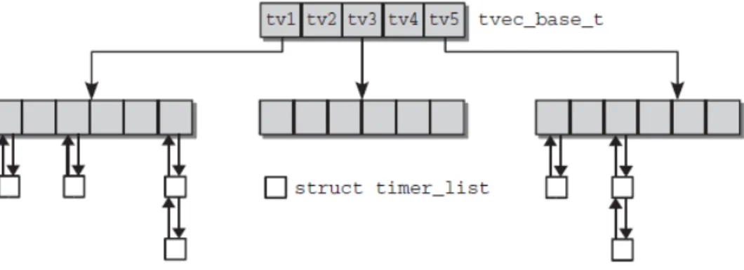
Figure 2.8: Data structures for managing timers

baseis a pointer to a central structure in which the timers are sorted on their expiry time. This

tvec_basestructure exists for each processor of the system; consequently, the CPU upon which the timer runs can be determined usingbase.

After the creation of the timer and the initial setup, one must specify the fields of thetimer_list

structure, and activate it with theadd_timerfunction (timer.h), adding it to a linked list where all the timers are stored. But because simply stringing together alltimer_listinstances is not satisfactory in terms of performance, the kernel needs data structures to manage all timers regis-tered in the system to permit rapid and efficient checking for expired timers at periodic intervals and not consume too much CPU time.

The kernel creates 5 different groups within thetvec_basestructure, into which the timers are classified according to their expiry time,expires. The basis for grouping is the main array with five entries whose elements are again made up of arrays. The five positions of the main array sort the existing timers roughly according to expiry times, so the kernel can limit itself to checking a single array position in the first group because this includes all timers due to expire shortly. Figure2.8shows how timers are managed by the kernel.

The first group is a collection of all timers whose expiry time is between 0 and 255 (or 28_{) ticks.}

The second group includes all timers with an expiry time between 256 and 28+6−1 = 214_{−1 ticks.}

The range for the third group is from 214to 28+2∗6− 1, and so on.

Typically, timers are run fairly close to their expiration, however they might be delayed until the first timer tick after their expiration. Consequently, timers cannot be used to implement any sort of real-time processing, so timers with accuracy better than 1 jiffy are needed. However low-resolution timersare useful for a wide range of situations and deal well with many possible use cases.

2.2.2.2 High-resolution Timers

For many applications, a timer resolution of several milliseconds, typical of low resolution timers, is not good enough. The hardware presented in the previous section provides means of much more precise timing, achieving nominally resolutions in the nanosecond range. During the development

(40)

Figure 2.9: Overview of the generic time subsystem

of kernel 2.6, an additional timer subsystem was added allowing the use of such timer sources. The timers provided by the new subsystem are conventionally referred to as high-resolution timers.

The mature and robust structure of the old timer subsystem did not make it particularly easy to improve while still being efficient, and without creating new problems. As we’ve seen before, to program a timer chip to interrupt the kernel at higher frequencies is not feasible due to the tremendous overhead [24]. The core of the high-resolution timer subsystem of the kernel can be found in kernel/time/hrtimer.c.

First, some concepts of the generic time subsystem, how does high-precision timekeeping is achieved in the kernel must be understood. The generic time framework provides the founda-tions for high-resolution timers, and is reused by low-resolution timers. In fact, in recent kernels low-resolution timers are implemented on top of the high-resolution mechanism. The generic timekeeping code that forms the basis for high-resolution timers is located in several files in ker-nel/time. Figure2.9[13] provides an overview of the generic time system.

There are three mechanisms that form the foundation of any kernel task related with time, each of them represented by a special data structure [25]:

• Clock Sources (defined by struct clocksource) - Provides a basic timeline for the system that tells where it is in time. Each clock source offers a monotonically increasing counter that ideally never stops ticking as long as the system is running, with a variable accuracy depending on the capabilities of the underlying hardware.

• Clock event devices (defined bystruct clock_event_device) - Allow for register-ing an event to happen at a defined point in time in the future. They take a desired time specification value and calculate the values to poke into hardware timer registers.

• Tick Devices (defined bystruct tick_device) - A wrapper aroundstruct clock _event_devicewith an additional feature that provide a continuous stream of tick events that happen at regular time intervals.

(41)

The kernel declares theclocksourceabstraction, in the linux/clocksource.h file, as a mean to interact with one of the hardware counter possibilities present in the machine [26].

struct clocksource { const char *name; struct list_head list; int rating;

cycle_t (*read)(struct clocksource *cs); int (*enable)(struct clocksource *cs); void (*disable)(struct clocksource *cs); u32 mult;

u32 shift;

unsigned long flags; ...

};

nameestablishes a human-readable name for the source, andlistis a standard list element that connect all available clock sources on a standard kernel list.

ratingspecifies the quality of the clock, between 0 and 499 to allow the kernel to select the best possible one. On modern Intel and AMD architectures, usually the TSC is the most accurate device, with a rating of 300, but the best clock sources can be found on the PowerPC architecture where two clocks with a rating of 400 are available.

readis a pointer to the function to read the current cycle value of the clock. The timing basis of this returned value is not the same for all clocks, so the kernel shall provide means to translate the provided counter into a nanosecond value. Since this operation may be invoked very often, doing this in a strict mathematical sense is not desirable: instead the number is taken as close as possible to a nanosecond value using only the arithmetic operations multiply and shift with the value ofmultandshiftfield members.

The field flagsofstruct clocksource specifies a number of flags that characterizes the clock with more detail.

Finally,enableanddisable, as the name suggests, are function pointers to allow the ker-nel to make the clock source available, or not. The machine’s clock sources made available by the kernel can be seen in the /sys/devices/system/clocksource/clocksource0/available_clocksource Linux file.

(42)

Theclock_event_devicestructure deals with the time at which it is supposed to generate an interrupt. It is defined in the include/linux/clockchips.h file:

struct clock_event_device {

void (*event_handler)(struct clock_event_device *);

int (*set_next_event)(unsigned long evt,

struct clock_event_device *);

int (*set_next_ktime)(ktime_t expires,

struct clock_event_device *); ktime_t next_event; u64 max_delta_ns; u64 min_delta_ns; u32 mult; u32 shift;

enum clock_event_mode mode;

unsigned int features;

void (*broadcast)(const struct cpumask *mask);

void (*set_mode)(enum clock_event_mode mode,

struct clock_event_device *);

const char _*name;

int rating;

int irq;

const struct cpumask *cpumask;

struct list_head list;

... };

The meaning of each field is described in the kernel code, but some key elements are to be highlighted.

max_delta_nsandmin_delta_nsspecify a range of values in nanoseconds in which the event shall take place with respect to the current time, characterizing the delay at each the event can be generated.

event_handlerpoints to the function that is called by the hardware interface code to pass clock events on to the generic layer.

cpumaskspecifies for which CPU’s the event device works. A simple bitmask is employed for this purpose. Local devices are usually only responsible for a single CPU.

next_eventstores the absolute time of the next event. This type of variable,ktime_t, is the data type used by the generic time framework to represent time values. This time representation consists of a 64-bit quantity independently of the architecture, and the manipulation of this objects, as well as the conversion to other time formats, must be made by auxiliary functions defined by the kernel in ktime.h file.

featurescharacterizes the event device, as a bit string. For example, CLOCK_EVT_FEAT _PERIODICidentifies a clock event device that supports periodic events, as well asCLOCK_EVT _FEAT_ONESHOT marks a clock capable of issuing one-shot events, that happen exactly once.

(43)

Most clocks allow both possibilities, but it can only be in one of them at a time, defined inmode, and theset_modefunction pointer is used to set the current mode of operation.

The next event in which event_handler is called to be triggered is configured in the

set_next_eventfunction, which in turn setsnext_eventusing a clocksource delta, or with

set_next_ktimethat uses a directktime_tvalue.

But there is no need to call these functions directly to set the mode and next event, as the kernel offers auxiliary functions for these tasks, defined in kernel/time/clockevents.c:

void clockevents_set_mode( struct clock_event_device *dev, enum clock_event_mode mode)

int clockevents_program_event( struct clock_event_device *dev, ktime_t expires, bool force)

Note that each clock event device only has one event programmed, so to manage multiple events, after the execution of the handler of one event, the kernel calculates how much time is left to the next event, and program the clock event device to generate an interrupt at that time. This is analogous to a situation where a family uses only one alarm clock to wake up all people at different times: the person that wakes up first needs to re-program the alarm clock to the next person’s wake up time.

Although clock devices and clock event devices are formally unconnected at the data structure level, some time hardware chips support both interfaces.

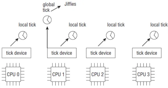
Besides these two concepts, the kernel distinguishes between two types of clocks, as we can see in figure2.9:

• A global clock, that is responsible to update the jiffies value, the wall time and the system load statistics.

• One local clock per CPU, that allows process accounting, profiling and most importantly, high-resolution timers.

Note that high-resolution timers only work on systems that provide per-CPU clock sources. The extensive communication required between processors would otherwise degrade system perfor-mance too much as compared to the benefit of having high-resolution timers.

After discussing the generic time framework, the implementation of high-resolution timers can be reviewed. These timers are distinguished from low-resolution timers in two aspects: first, the HR (High-Resolution) timers are time-ordered on a red-black tree, and second they are indepen-dent of periodic ticks, employing nanosecond time stamps instead of a time specification based on jiffies.

Since low-resolution timers are implemented on top of the high-resolution mechanism, the generic part of the high-resolution timers framework will always be built into the kernel even if support for them is not explicitly enabled. Nevertheless the supported resolution is not any better. This means that even kernels that only support low resolution contain parts of the high-resolution framework, which can sometimes lead to confusion.

(44)

HR timers must be bound to one of two clock bases:

• CLOCK_MONOTONIC, maintained by the operating system from the system’s boot timer, it resembles the tick count and it is guaranteed to always run monotonously in time. It is the preferred clock for calculating the time difference between events [27].

• CLOCK_REALTIME can jump forward and backwards. It represents the system’s best guess of the real time-of-day and it can be modified by a user with the right privileges. Currently there are two more clock bases in the kernel: the CLOCK_BOOTTIME that is idential to CLOCK_MONOTONIC, except it also includes any time spent in suspend [28], and CLOCK_TAI, since 3.10, which was managed by the NTP code before, and was moved into the timekeeping core to provide a TAI (International Atomic Time) based clock [29].

Each of these clock bases is an instance of struct hrtimer_clock_base, which is equipped with a red-black tree that sorts all pending HR timers, and specifies its type, resolu-tion, and the function to read its current time. The function to read the CLOCK_MONOTONIC is ktime_get()and to read the CLOCK_REALTIME, thektime_get_real() function is used, both returning aktime_ttime stamp value. There is a data structure with all these clock bases for each CPU in the system, namedstruct hrtimer_cpu_base. Both these structures are in hrtimer.h file.

The HR timer itself is specified byhrtimerdata structure provided by the kernel, defined in the same file:

struct hrtimer {

struct timerqueue_node node;

ktime_t _softexpires;

enum hrtimer_restart (*function)(struct hrtimer *);

struct hrtimer_clock_base *base;

unsigned long state;

#ifdef CONFIG_TIMER_STATS int start_pid; void *start_site; char start_comm[16]; #endif };

struct timerqueue_nodespecifies the node used to keep the timer on the red-black tree, and also the absolute expiry time in the hrtimers internal representation. basepoints to the timer base associated.

state is the currently state of the timer, that can be inactive, waiting for expiration (en-queued), executing the callback function, pending, i.e. has expired and is waiting to be executed, or migrated to another CPU.

start_commandstart_pid are respectively the name and the pid (processor identifica-tion) of the task which started the timer, for timer statistics.

(45)

The most important field is obviously the timer expiry callbackfunctionthat can return two possible values:

enum hrtimer_restart {

HRTIMER_NORESTART, /* Timer is not restarted */

HRTIMER_RESTART, /* Timer must be restarted */

};

If the callback returnsHRTIMER_NORESTART, the timer will simply eliminated from the sys-tem after expires. In order to the timer to be restarted, the callback must set the new expiration time on the hrtimer parameter and the return value must beHRTIMER_RESTART. The kernel provides an auxiliary function to forward the expiration time of a timer:

extern u64

hrtimer_forward(struct hrtimer *timer, ktime_t now, ktime_t interval);

Usuallynowis set to the value returned byhrtimer_clock_base->get_time(), and for that reason,hrtimer_forward_now(struct hrtimer *timer, ktime_t interval)

was created, that already does that.

The new expiration time must lie pastnow, sointervalis added to the old expiration time the times necessary to make that true. The functions returns the number of times thatinterval

had to be added to the expiration time to exceednow. This makes possible to track how many periods were missed if periodic execution of the function is desired, and respond to the situation.

To actually set and use the timers, there is a well defined interface provided by the kernel in hrtimer.h[30].

In order to use ktime_t time values, ktime_set(long secs, long nanosecs) is used to declare and initialize them. Several other auxiliary functions exist to handle this kind of variables, like to add or subtract time values and convert to other time representations.

A newstruct hrtimeris initialized withhrtimer_init(struct hrtimer *timer, clockid_t which_clock), in whichclockis the clock base to bind the timer to, andmode

specifies if time values are to be interpreted as absolute or relative to the current time, with the constantsHRTIMER_MODE_ABSandHRTIMER_MODE_REL, respectively.

The next step is to define thefunctionpointer to the callback, since this is the only field that is not set with the API funtions, andhrtimer_startis used to set the expiration time of a timer, declared before, and starts it. Thehrtimercode implements a shortcut for situations where the sole purpose of the timer is to wake up a process on expiration: if the function is set toNULL, the process whose task structure is pointed to by thedatawill be awakened.

If periodic execution of the callback function is desired, after the application code to be ex-ecuted in it,hrtimer_forwardmust be used, processing the returned overrun eventually, and returnHRTIMER_RESTART. Timers can be canceled and restarted withhrtimer_canceland

hrtimer_restartrespectively. hrtimer_try_to_cancelmay also be used with the par-ticularity that it returns -1 if the timer is currently executing and thus cannot be stopped anymore.

(46)

When an interrupt is raised by the clock event device responsible for HR timers, the event handler that is called is hrtimer_interrupt. Assuming that the high-resolution timers will run based on a proper clock with high-resolution capabilities that is up and running, and that the transition to high-resolution mode is completely finished (since only low-resolution will be available at boot), this function selects all expired timers in the tree, calls the handler function associated with it, and reprograms the hardware for the next event depending on the return value of the handler function, while changing dynamically thestateof the timer. This is done for each clock base, iteratively.

Concluding, in this section the high resolution timers were reviewed, as well as their imple-mentation. In the next section, the last one of this overview of the Linux time management, shows some top-level application interfaces to use high resolution timer in user-space.

2.2.2.3 Timer APIs

These HR timers are used for heavily clock-dependent applications. In order to support user-level applications, such as animations, audio/video recording and playback, and motor controls, the Linux kernel provides different APIs, i.e. system call interfaces, for using high resolution timers. The most important are the following [31]:

• timerfd - An interface defined in fs/timerfd.c that presents POSIX timers as file descriptors and waiting for the timer to expire consists of read from it, always returning an unsigned 64-bit value representing the number of timer events since the last read, which should be one if all is going well. If it is more than one then some events have been missed.

• POSIX timers - Implemented in kernel/posix-timers.c, these timers generate signals indi-cating the expiration time, and the start of the next period in case of periodic operation. One must wait for the signal to arrive withsigwait()and the missed events can be detected using the functiontimer_getoverrun(), which returns zero if none were missed. • setitimer - A system call whose implementation rest in kernel/itimer.c that installs interval

timers similar to POSIX clocks except that it is hard coded to deliver a signal at the end of each period. The time out is passed in a structitimerval(time.h) which contains an initial time out, it_value, and a periodic time out in it_intervalwhich is reloaded intoit_valueevery time it expires.

When itimers are used there are three options to distinguish how elapsed time is counted or in which time base the timer resides, specified inwhichparameter insetitimer:

• ITIMER_REALfires aSIGALRMsignal after a specified real time measured between acti-vation of the timer and time-out.

• ITIMER_VIRTUALmeasures only time consumed by the owner process in user mode, and draws attention to itself by triggering aSIGVTALRMsignal upon time-out.

• ITIMER_PROFcalculates the time spent by the process both in user and kernel mode,and the signal sent at time-out isSIGPROF.

(47)

2.3 Clock synchronization algorithms 27

2.3 Clock synchronization algorithms

This section focus on how processes can synchronize their own clocks.

In a centralized system time , where a centralized server will dictate the system time, time is unambiguous. It does not matter much if this clock is off by a small amount to the real time. Since all processes will still be internally consistent.

But with multiple CPU’s, each with its own clock, it is impossible to guarantee that the crystal oscillators don’t have a drift, and differ after some amount of time even when initially set accu-rately. In practice, all clocks counters will run at slightly different rates. This clock skew brings several problems that can occur and several solutions as well, some more appropriate than others in certain contexts.

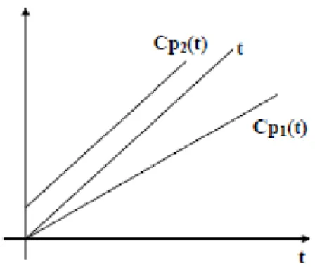
All the algorithms have the same underlying system model. Each processor is assumed to have a timer that causes a periodic interrupt H times a second, but real timers do not interrupt exactly H times per second [32].

Figure2.10show a slow, a perfect, and a clock with constant offset. The most important clock parameters to measure a clock synchronization, are:

• Accuracy α : |Cpi(t) − t| ≤ α for all i and t

• Precision δ : |Cpi(t) −C pj(t)| ≤ δ for all i, j, t

• Offset : Difference between C pi(t) and t

• Drift : Difference in growing rate between C pi(t) and t

(48)

2.3.1 Network Time Protocol

A common approach in many protocols, is for a client to read a server’s clock and compensate for the error introduce by message delay.

Figure 2.11: Getting the current time from a time server.

In this protocol, (see figure2.11), A will send a request to B, timestamped with value T1. B,

in turn, will record the time of receipt T2(taken from its own local clock), and returns a response

timestamped with value T3, and piggybacking the previously recorded value T2. Finally, A records

the time of the response’s arrival, T4. Let us assume that the propagation delays from A to B is

roughly the same as B to A, meaning that T2− T1≈ T4− T3. In that case, A can estimate its offset

relative to B as stated in expression2.5.

θ = (T2− T1) + (T3− T4)

2 (2.5)

There are many important features about NTP, of which many relate to identifying and masking errors, but also security attacks. NTP is known to achieve worldwide accuracy in the range of 1-50 msec. The newest version (NTPv4) was initially documented only by means of its implementation, but a detailed description can be found in [33].

2.3.2 The Berkeley Algorithm

In contrast, in Berkeley UNIX, a time server is active, polling every machine from time to time to ask what time it is there, computing the answers to tell the other machines to advance their clocks to the new time or slow their clocks down until some specified reduction has been achieved, since it is not allowed to set the clock backwards.

In figure2.12we can see the time server (actually, a time daemon) telling the other machines its own time and asks for theirs. They respond with how far ahead or behind they are and the server computes the average and tells each machine how to adjust its clock.

This algorithm is more suitable for systems that pursue only that all machines agree on the same time, and not a correct absolute value of the clocks, i.e. internal clock synchronization rather than external clock synchronization.